formation which is common to optimizations like common subexpression .... The PVS ground evaluator consists of a PVS to Common Lisp translator, an.
A PVS based Framework for Validating Compiler Optimizations Aditya Kanade
Amitabha Sanyal
Uday Khedker
Dept. of Computer of Science and Engineering, IIT Bombay. E-mail: {aditya,as,uday}@cse.iitb.ac.in Abstract An optimization can be specified as sequential compositions of predefined transformation primitives. For each primitive, we can define soundness conditions which guarantee that the transformation is semantics preserving. An optimization of a program preserves semantics, if all applications of the primitives in the optimization satisfy their respective soundness conditions on the versions of the input program on which they are applied. This scheme does not directly check semantic equivalence of the input and the optimized programs and is therefore amenable to automation. Automating this scheme however requires a trusted framework for simulating transformation primitives and checking their soundness conditions. In this paper, we present the design of such a framework based on PVS. We have used it for specifying and validating several optimizations viz. common subexpression elimination, optimal code placement, lazy code motion, loop invariant code motion, full and partial dead code elimination, etc.
1. Introduction A compiler optimizer analyzes and transforms programs to improve their run-time behavior. This allows programmers to focus on functionality of programs without having to bother about efficiency of the generated code. Optimizers have therefore become an integral part of the modern compilers. However, a mistake in the design or the implementation of an optimizer can proliferate in the form of bugs in the softwares compiled through it. Like any critical software, it is desirable to have a verified implementation of optimizers. However, the verification techniques are not sophisticated enough to verify complex softwares like optimizers mechanically. The issue of soundness of optimizers is therefore addressed at two levels: (1) One time guarantees are obtained at the design level by verifying optimization specifications and (2) run-time guarantees are obtained at the implementation level by validating optimizations performed.
Both these approaches involve proofs of semantic equivalences between the input and the optimized programs. However, they are usually tedious. Even in the case of validation where semantic equivalence is to be shown for a particular execution, it cannot be accomplished with ease. This complexity can be conquered by taking advantage of the fact that optimizations with similar objectives employ similar program transformations. For example, “replacement of some occurrences of an expression by a variable” is a transformation which is common to optimizations like common subexpression elimination, lazy code motion, loop invariant code motion, and several others whose aim to avoid unnecessary recomputations of a value. In [4], we have identified a set of common transformation primitives which can be used to specify a large class of optimizations by sequential composition. For each primitive, we have defined soundness conditions which guarantee that the transformation is semantics preserving. The program points which satisfy soundness conditions are called safe application points. If the transformation is applied to a subset of these points, the resulting program is semantically equivalent to the input program. Proving sufficiency of soundness conditions for semantics preservation under the respective transformation is a one time affair. Since the primitives are small-step transformations, these proofs are much easier than similar proofs for optimizations. This approach reduces proving the soundness of an optimization to showing that the soundness conditions of the underlying primitives are satisfied on the versions of the input program on which they are applied. This is much simpler than directly proving semantics preservation for an optimization. This approach works at the design level by verifying soundness of specifications. In [4], we have additionally proposed how this technique can also be used for reducing efforts required for validating actual implementations. An obvious approach is that of validating against a specification. First a specification of an optimizer is proved sound and then their inputs and outputs are matched on a run-by-run basis. There is however a simpler approach of validating against a trace which does not even require proving soundness of specifications.
P α abstraction function M1
(instrumented) trace τ =
T1 (π1 ); . . . , Tk (πk );
Ti (πi )
• A trusted framework for simulating and validating optimization specifications. Soundness conditions model global program properties and are defined in a temporal logic. We have given boolean matrix algebraic definitions of temporal operators and transformation primitives. These definitions can be evaluated in the PVS ground evaluator.
α Mk+1
SIMULATOR
Mi
We summarize the contributions of this work as follows:
P′
OPTIMIZER
Mi+1
πi ⊆ ϕi (Mi )?
• Automatic generation of verification conditions. Besides the contribution to optimization validation, our work is also interesting in its use of PVS. One such contribution is a utility to automatically generate verification conditions by probing the internal representation of PVS theories. If the verification conditions are satisfied on a program, the optimization preserves semantics of the program. These conditions also constitute the proof obligations for verifying the soundness of the optimization specification.
Figure 1. Validating against a trace
An optimizer can be instrumented to generate a trace τ of its execution on a program P as a sequence of appropriately instantiated primitives T1 , . . . , Tk as shown in Fig. 1. The program points to which these primitives are applied are π1 , . . . , πk . The abstract representation of the input program is M1 . The transformation Ti (πi ) is applied on the abstraction Mi and results in the abstraction Mi+1 . The optimized program P ′ is semantically equivalent to the input program P if (1) the abstract representation of P ′ matches the abstraction Mk+1 obtained by simulating the trace on the abstraction M1 and (2) the soundness conditions ϕi of the transformation primitives Ti are satisfied on the abstractions Mi , that is the actual application points πi are a subset of the safe application points of the primitive Ti on the abstraction Mi . Similar to verification, this validation scheme also takes advantage of common patterns of transformations and of semantic equivalence proofs. This scheme does not directly check semantic equivalence of the input and the optimized programs and is therefore amenable to automation. The soundness of the validation scheme in Fig. 1 is subject to the soundness of the abstraction function and the simulation environment. The instrumented optimizer can potentially generate an inconsistent trace. However, since the abstraction obtained by simulating the trace is matched with the abstraction of the optimized program, the inconsistency is detected. We have shown separately on paper that the transformation primitives preserve semantics if their soundness conditions are satisfied. In these proofs, we use some properties of the transformation primitives. For the purpose of this paper, we assume that the definitions of the primitives encoded in the validation framework satisfy the properties used in the proofs of semantics preservation. In this paper, we present the design of a simulation framework based on the ground evaluator of the trusted PVS system. We have specified and validated several optimizations in our framework. These specifications are not only executable but having been written in PVS are also amenable to formal verification.
• Validation of several optimizations. As a proof of concept, we have specified several optimizations. We have simulated them on various programs and have validated their simulation traces. The optimizations that are considered include common subexpression elimination, optimal code placement, lazy and loop invariant code motion, full and partial dead code elimination, etc. This also demonstrates that our framework is suitable for rapid prototyping of optimizations. The rest of the paper is organized as follows: Section 2 describes the PVS system and the architecture of the validation framework. Section 3 explains the specification mechanism. Sections 4–5 discuss the basic theories in the framework. Section 6 explains the simulation and validation mechanism. Section 7 discusses related work. Section 8 concludes and proposes future directions.
2. Architecture of the Validation Framework The Prototype Verification System (PVS) [10] is an interactive system used for developing and verifying formal specifications. In our earlier work [4], we have explained its use in verification of optimization specifications. PVS also provides a useful facility of expression evaluation. We can therefore use PVS as an integrated environment for both verification and validation of optimization specifications. Fig. 2 shows the architecture of the PVS based validation framework. The unshaded boxes denote the components of PVS and the shaded boxes denote the extensions that we have added to the PVS core. 2
The Validation Framework. We extend the prelude with two libraries: TTL and OVerification. These libraries are collections of theories formulating the basic concepts required for specifying optimizations. The TTL library contains definitions of temporal operators and graph transformations. TTL is an abbreviation for the Temporal Transformation Logic which is used in the verification of optimization specifications [4]. The temporal operators and the graph transformations are defined in a boolean matrix algebra. This novel formulation facilitates simple algebraic proofs of soundness of the TTL inference rules. Additionally, our formulation of the boolean matrix algebra is operational and written completely in the executable fragment of the PVS language. This makes model checking of temporal formulae and simulation of graph transformations possible in the PVS ground evaluator. The OVerification library defines an abstraction of programs which is based on control flow graph representation of three–address code. It also builds the vocabulary for writing specifications of optimizations by defining local data flow properties and transformation primitives. The primitives define the content and the control flow of the transformed program in terms of the input program. The control flow transformations are expressed in terms of the graph transformations defined in the TTL library. The theories in the OVerification library also define the soundness conditions of the transformation primitives. All these definitions are written in the executable fragment of the PVS language. These definitions are operational and hence can be simulated directly in the PVS ground evaluator. We have developed a utility called VC generator to generate verification conditions from specifications. Like other components of the PVS system, it is also hooked into the Emacs interface. It probes the internal representation of PVS specifications created by the parser and the typechecker. It identifies usage of programs transformations and emits appropriate verification conditions in a separate PVS file. These conditions are evaluated in the ground evaluator to validate a particular optimization run. These conditions also form the proof obligations for the verification of the optimization specification.
PVS Emacs Interface P & TC
PC
GE
VC Generator
Prelude theories PVS language
OVerification
PVS Core
Extensions
TTL
Figure 2. Schematized Architecture of the PVS based Validation Framework
Overview of the PVS system. In this paper, we present the validation framework that uses the PVS ground evaluator (GE) for simulating specifications. Readers do not have to know the entire PVS proof engine to understand this paper. Our specification language is based on the PVS language and we explain it as and when needed. Optimization specifications are written as PVS theories in the PVS Emacs interface and are saved in files with .pvs extension. These specifications are written in the PVS language extended with a specialized vocabulary. The PVS language is based on higher-order logic, i.e., functions are first-class objects and quantification over general objects is supported. It is a typed language and supports powerful typing mechanisms like subtyping and dependent typing. PVS has a set of predefined theories called prelude. The theories in the prelude define many basic concepts and serve as building blocks for user defined theories. All specification processing functionalities of PVS are hooked into the Emacs interface. Upon starting a PVS session, the customized Emacs interface is loaded which in turn loads the PVS Lisp image. The parser checks theories for syntactic consistency and builds an internal representation that is used by other components of PVS. The typechecker analyzes theories for semantic consistency and adds semantic information to the internal representation built by the parser. The parser and the typechecker are denoted by (P & TC) box in Fig. 2. PVS provides an interactive proof checker (PC) for deriving proofs of formulae declared in a specification.
3. Specifying Optimizations
The PVS ground evaluator (GE) is an environment in which ground expressions, i.e., executable definitions applied to concrete data, are evaluated. The PVS ground evaluator consists of a PVS to Common Lisp translator, an interactive read-eval-print interface, and a proof rule [7]. The unexecutable constructs in PVS are uninterpreted symbols, non-bounded quantification, and higher-order relations. The PVS ground evaluator can be used for rapid prototyping and validation of specifications.
In this section, we discuss the specification mechanism. We have specified several optimizations including common subexpression elimination, lazy code motion, loop invariant code motion, full and partial dead code elimination, etc. We use optimal code placement [13] as an example. We first present some local data flow properties and then explain the specification mechanism for analyses and transformations. 3
3.1. Local Data Flow Properties
1
We consider control flow graph based abstraction of three–address code. The control flow graph is denoted by cfg. Its transition relation is given as a boolean adjacency matrix. It has a single entry and a single exit which are denoted by a list of boolean values each with only the elements at the appropriate positions set to true. A list of statements L gives the contents of a program. The ordering of the statements in the list implicitly determines the program points to which they correspond. We consider four kinds of statements: skip, assignment, conditional branching, and halt. Unconditional branching is modeled by directed edges. A local data flow property defines statement-level conditions. Value of a local data flow property is given by a list of booleans. The element corresponding to a program point is set to true only if the property is satisfied by the statement at the program point. We define several local data flow properties found in the literature as part of the OVerification library. These properties can be used for specifying optimizations. Below we summarize the local data flow properties used in this paper. Consider a program denoted by prog.
2 x = a+b
3
4 5 7 y = a+b
6 9
8 10 y = a + b 11 x = a + b 12 x = a + b
Nec nodes Ear nodes
13
Figure 3. Optimal Code Placement Analysis
The optimization should however preserve semantics of the program being transformed. The insertions of computations of a+b should not give rise to computation of new values along any paths. Further, the original computations of a+b should only be replaced by a variable which will evaluate to the same value as the expression a+b. We now explain the required program analyses. An expression can be placed safely at a program point if along all forward paths from the point it is computed and none of its operands are assigned before the computation. This is specified as Nec (necessity) analysis in Fig. 4. It takes a program prog and an expression e and returns a list of booleans. If an element in the list is true then the property is satisfied at the corresponding program point. Nec is a global data flow property, i.e., it relates data flow information along control flow paths. We use computational tree logic with branching past (CTLbp ) [5] for specifying global data flow properties. A Kripke structure forms a model for formulae of CTL bp . It consists of a set of states, a binary transition relation over the states, a set of atomic propositions, and a labeling function which associates labels with states. A program abstraction together with local data flow properties can be seen as a Kripke structure. The program points (or nodes) form the states of the Kripke structure. The control flow transition relation defines the transition relation of the Kripke structure. Local data flow properties and their values determine the set of atomic propositions and the labeling function respectively. CTLbp is a branching-time temporal logic. A state in its model can have multiple predecessors and multiple suc-
• Mod(prog,e) holds at a program point if an operand of the expression e is assigned at the program point. • Antloc(prog,e) holds at a program point if the expression e is computed at the program point. • Transp(prog,e) holds at a program point if no operand of the expression e is assigned at the program point. • Comp(prog,e) holds at a program point if the expression e is computed at the program point and none of its operands is assigned at that point. • Use(prog,v) holds at a program point if the variable v is an operand of the expression computed at the point. • Def(prog,v) holds at a program point if the variable v is assigned at the program point. • AssignStmt(prog,v,e) holds at a program point if the statement at the program point is v = e.
3.2. Specifying Analyses Consider the program shown in Fig. 3. The nodes represent the program points and the edges represent the flow of control. The expression a+b is computed in nodes 2, 7, 10, 11, and 12. Several of these nodes share common execution paths. By placing computations of a+b only in certain common dominators of these nodes, the number of computations of a+b in the program can be reduced. 4
Nec(prog, e) : list[bool ]
= AW(prog‘cfg, /(Mod(prog, e) + prog‘exit) , Antloc(prog, e))
Ear(prog, e) : list[bool ]
= /(AY(prog‘cfg, AS(prog‘cfg, /(Mod(prog, e)), Nec(prog, e) − Mod(prog, e)))) = Ear(prog, e) ∗ Nec(prog, e)
Ocp(prog, e) : list[bool ]
Figure 4. Specification of OCP Analyses cessors. In CTLbp , past is finite whereas future is infinite. We define the CTLbp operators in a modal algebra. These definitions are developed as part of the TTL library. In our notation, an operator takes the control flow graph of a program as an additional (first) parameter. Definitions of the CTLbp operators are explained in section 4.1. The property Nec is defined using the weak until operator AW and reads as follows: Along all forward paths, the expression e is not Mod-ified and the program exit is not encountered until an Antloc computation of the expression e is encountered. For an infinite path due to a program loop, the expression e is not Mod-ified and the program exit is not encountered, ever. The “/” operator is negation extended to boolean lists and matrices. The “+” operator is disjunction extended to boolean lists and matrices. Fig. 3 shows the program points which satisfy the Nec property for a+b. A program point is earliest if the expression e cannot be moved to its predecessors without violating the safety (Nec) property. This property is defined as Ear analysis. The operator AY reads as “for all predecessors”. The operator AS is the counter part of AW in the backward direction. The property Ear reads as follows: It is not the case that for all backward paths starting with the predecessors, the expression e is not Mod-ified until a program point satisfying Nec but not Mod is reached. Fig. 3 shows the program points which satisfy the Ear property for a+b. The placement points are identified by the property Ocp. These points satisfy the Nec and Ear properties. The “∗” operator is conjunction extended to boolean lists and matrices.
1 14 t = a + b 2
x=t
3
4 15 t = a + b 5 7
y=t
6
8
9
10
y=t
x=t
12
11
x=t
New nodes Optimized
13
Figure 5. Optimized Program The optimization is specified formally as the function
3.3. Specifying Transformations
OCP Transformation as shown in Fig. 6. It takes a program prog1 and an expression e and returns the optimized version of prog1. For readability, we have simplified the
The optimal code placement optimization is performed in three steps: (1) Insert a new predecessor each to the Ocp points, (2) Assign the expression e to a new variable t at the newly inserted points, and (3) Replace all the original computations of the expression e (i.e., except those inserted in the second step) by the variable t . Fig. 5 shows the optimized version of the program in Fig. 3. We define the small-step transformations corresponding to the above steps as transformation primitives. They are also used in specifications of other optimizations with similar transformation patterns, e.g., lazy code motion, loop invariant code motion, etc. We discuss the definitions of these transformation primitives in section 5.1.
syntax slightly. If the expression e is not computed in prog1, the optimization returns prog1 as it is. The function Expressions gives the expressions computed in a program. The program points satisfying the Ocp property in prog1 are denoted by ocppoints. The program points where the expression e is computed (Antloc) in prog1 are denoted by antloc. IP is a transformation primitive which takes a program and a set of program points and inserts a new predecessor to each of them. In order to keep the specifications executable, we represent a set of program points by a list of booleans. If an element in the list is true then the program point at the corresponding location is a member of the set. The new program points are distinct from the program points of the 5
as a boolean adjacency matrix T. The atomic propositions are generalized to predicates over states and their valuations are lists of boolean values. A value true at a particular location in the list corresponds to the predicate being true at the corresponding state. We define the CTLbp operators in a boolean matrix algebra (also known as a modal algebra) and the mu-calculus. Consider a graph G and a proposition phi. The temporal formula EX(G,phi) holds at a state if the proposition phi holds at some successor of the state. Consider the column matrix corresponding to the proposition phi. The value of EX(G,phi) is obtained by multiplying the transition relation G‘T with the column matrix as defined in (1). The boolean matrix multiplication is denoted by the symbol “#”.
OCP Transformation(prog1, e): Program = IF member(e, Expressions(prog1)) THEN LET ocppoints = Ocp(prog1, e), antloc = Antloc(prog1, e), prog2 = IP(prog1, ocppoints), newpoints = prog2‘cfg‘ns − prog1‘cfg‘ns, t = NEWVAR(prog2), prog3 = IA(prog2, newpoints, t, e) IN RE(prog3, antloc, t) ELSE prog1 ENDIF
Figure 6. Spec. of OCP Transformation input program. Here, it returns the program prog2. In Fig. 5, the newly inserted predecessors to ocppoints (nodes 2 and 5) are nodes 14 and 15. The new program points contain skip statements whereas the statements at the other points remain unchanged with respect to the program prog1. Let newpoints be the new program points inserted by the first transformation. Let t be a new variable with respect to prog2. IA is a transformation primitive which takes a program, a set of program points, a variable, and an expression and inserts a statement assigning the expression to the variable at the given points. Here, it inserts t = e at newpoints. The transformed program prog3 is structurally same as prog2. In Fig. 5, prog3 will have the statement t = a+b at nodes 14 and 15. Finally, all the original computations of the expression e are replaced by the variable t. RE is a transformation primitive which takes a program, a set of program points, and a variable and replaces the expressions computed at the given points by the variable. Here, it takes the program prog3 and replaces the expressions computed at the antloc points by the variable t. Fig. 5 shows the optimized program obtained by simulating OCP Transformation on the program shown in Fig. 3 for the expression a+b.
EX(G,phi) = G‘T # phi
(1)
This results in a column matrix. For simplicity, we use lists and column matrices interchangeably. If A and B are two boolean matrices of suitable dimensions then b j) [A#B]ji = foldl(or, false, [A]i ∗ [B] where for a matrix Z, [Z]ji is (i, j)th element of Z, [Z]i is b is the transpose of Z. ith row, and Z The temporal formula EY(G,phi) holds at a state if the proposition phi holds at some predecessor of the state. By taking transpose of an adjacency matrix we get the graph with inverted edges. The value of EY(G,phi) is obtained by multiplying the transpose of the transition relation G‘T with the column matrix corresponding to phi as defined in (2). d EY(G,phi) = G ‘T # phi
(2)
The temporal formula AX(G,phi) holds at a state if the proposition phi holds at all the successors of the state. Similarly, AY(G,phi) holds at a state if phi holds at all the predecessors of the state. It does not hold at the program entry which has no predecessors. These are defined in (3) where “−” denotes boolean matrix subtraction.
4. Defining Temporal Operators and Graph Transformations
AX(G,phi) AY(G,phi)
We now present the theories in the TTL library. It defines temporal operators and a few basic graph transformations. Unlike our earlier formulations [4], these definitions are operational and written in the executable fragment of the PVS language. These can therefore be evaluated directly in the PVS ground evaluator.
= / (EX(G, /(phi))) = / (EY(G, /(phi))) − G‘entry
(3)
The weak until formula AW(G,phi,psi) holds at a state if along all forward paths phi holds until psi holds or phi holds forever. The past (or backward) until formula AS(G,phi,psi) is similar but interpreted in the backward direction. These are defined as greatest fixed points as follows:
4.1. Temporal Operators
AW(G,phi,psi) = nu (λ theta. psi + (phi ∗ AX(G,theta))) AS(G,phi,psi) = nu (λ theta. psi + (phi ∗ AY(G,theta)))
A Kripke structure serves as a model for temporal logic. In our formulation, a Kripke structure is represented by a directed graph, say G. Its transition relation is represented
where nu is the greatest fixed point operator and λ is the lambda operator. 6
4.2. Graph Transformations E
E
2 C b C
Np
1
3
Ei
Np
4 Ns
G
Ei Eo
2
G′
Figure 8. Insert Predecessors
5.1. Transformation Primitives The transformation primitive IP inserts a new predecessor to each program point in a given set. It is used in the first transformation of OCP Transformation in Fig. 6. The control flow graph of the transformed program is defined using the node addition transformation. Consider the graph G in Fig. 8. We want to insert a new node 4 as a predecessor to node 2. The transformed graph is G′ . The dashed arrows from the nodes of G′ to the nodes of G represent the correspondence C. The dashed arrows in the opposite direction represent the transpose of C. The incoming edges to node 2 in G form the matrix E. b − C#E#C b ) in (4) gives all the The term (C#G‘T#C ′ edges of G except the incoming edges to nodes 2 and 4. The matrix multiplication can be seen as composition of the arrows and the edges. For example, by following the dashed arrows from right to left, we go from node 1 of G′ to node 1 of G. We then follow the edge 1 to 3 in G. Finally, we follow the dashed arrows from left to right to get from node 3 of G to node 3 of G′ . This gives us the edge 1 to 3 in G′ . Similarly, other edges can be traced. The matrix Np maps the predecessors of node 2 in G (nodes 1 and 3) to node 4 of G′ . By following the dashed arrows from right to left and then following the Np arrows from left to right, we get the incoming edges Ei of node 4. The matrix Ns maps node 4 of G′ to node 2 of G. By tracing b arrows, we get the Eo edge 4 to 2. The newly Ns and C inserted node 4 contains a skip statement. The other transformations used in the specification of OCP Transformation are IA for “insert assignments” and RE for “replace expressions by a variable”. They change only the statements associated with the program points being transformed. These primitives are defined as updating of the statement list L of the input program.
b = G′ ‘T (4) b − C#E#C b )+ C#Np + Ns #C (C#G‘T#C | {z } | {z } Ei
3
1
We identify a few basic graph transformations viz. node addition, deletion, splitting, merging and edge addition and deletion. We now explain the node addition transformation. Consider a graph G. Let G′ be its transformed version. Let there be n nodes in G and m nodes in G′ . Consider an (m×n) correspondence matrix C that represents the correspondence relation between the nodes of G′ and G. Suppose two nodes u and v of G′ correspond respectively to nodes i and j in G. We want to add a new node w as a predecessor of j and a successor of i. By a new node, we mean that there is no node corresponding to it in G. We add an edge from u to w and an edge from w to v in G′ making w a predecessor of v and a successor of u. There is no edge between u and v. The other edges of G′ correspond to the edges of G. We call this transformation node addition. The correspondence (relation) C is required to be a partial and onto function, that is every node in G has exactly one corresponding node in G′ whereas a new node in G′ does not correspond to any node in G. The edges of G′ are defined in terms of the edges of G as follows:
Eo
where E is an (n×n) adjacency matrix where only the edge from i to j is marked true. Np is an (n×m) matrix which establishes the correspondence between node i and node w, i.e., only the element at (i, w) is true. Ns is an (m×n) matrix which establishes the correspondence between node w and node j, i.e., only the element at (w, j) is true. b ) gives all the edges of G′ correThe term (C#G‘T#C b ) gives the sponding to the edges of G. The term (C#E#C edges corresponding to the edge from i to j. If any such edge is present, it is removed because a new node is being added between i and j. The term Ei maps the edge from i to j to an edge from u to w. The term Eo maps the edge from i to j to an edge from w to v. This simple and concise definition of the node addition transformation is used for defining a variety of control flow transformations in the OVerification library viz. insertion of predecessors or successors and edge splitting.
5. Defining Transformation Primitives and their Soundness Conditions
5.2. Soundness Conditions The OVerification library defines control flow graph based abstraction of three–address code. It is explained in section 3.1. We now discuss the definitions of the transformation primitives and their soundness conditions which are developed as part of the OVerification library.
The transformation primitive IP does not introduce new execution paths in the transformed program. It only extends the existing paths. The new nodes contain skip statements and hence do not affect the program state. Therefore, 7
Available(prog,e) : list[bool ] Anticipatable(prog,e) : list[bool ] Dead(prog,v) : list[bool ] EqValue(prog,v,e) : list[bool ] SoundIA(prog, points, v, e) : bool
= AS(prog‘cfg, Transp(prog,e), Comp(prog,e)) = AW(prog‘cfg, Transp(prog,e) − phi’exit, Antloc(prog,e)) = AW(prog‘cfg, /(Use(prog,v)), Def(prog,v)) = AY(prog‘cfg, AS(prog‘cfg, Transp(prog,e) − Def(prog,v), AssignStmt(prog,v,e))) = Skips(prog,points) ∧ (points ≤ (Dead(prog,v) + EqValue(prog,e,v))) ∧ (points ≤ (Available(prog,e) + Anticipatable(prog,e)))
Figure 7. Soundness Conditions for the transformation primitive IA any application of the primitive preserves semantics. The soundness condition of IP is thus vacuously true. The soundness condition (SoundIA) of the primitive IA is given in Fig. 7. An application IA(prog, points, v, e) preserves semantics if (1) The statements at points in the program prog are skip statements (Skips). (2) The variable v is not used in the future unless redefined (Dead) or the variable v and the expression e have the same value at the point of insertion (EqValue). This ensures that wherever v is used, it has the same value in both the input and the transformed programs. (3) The expression e is already computed in the past (Availability) or will be computed in the future (Anticipatability). This ensures that the computation of e at the point does not result in any new value being computed along any path. The soundness condition of the primitive RE is defined as follows: Let p be a point in a set of program points points and e be the expression computed at p. An application RE(prog, points, v) at p preserves semantics if the variable v and the expression e have the same value (EqValue) at p. This ensures that the variable being assigned to at p gets the same value in both the input and the transformed programs. We have separately shown that if soundness conditions of a primitive are satisfied then the transformation preserves semantics. A sample proof is available in [4].
1. It installs the functions required for probing the internal representation of PVS declarations stored in the PVS Lisp image by invoking install-pvs-funs function. It then initializes global variables to be used for processing of the internal representation by sending the command (init-vars) to the PVS Lisp image via the function pvs-send-and-wait. pvs-send-and-wait is a function for synchronous inter-process communication between the Emacs Lisp and the PVS Lisp images. 2. It gets the name of the specification theory via get-theory-name function which stores the name in the variable theory-name. It then invokes the function get-opt-decl which probes the theory declaration using the PVS Lisp functions installed in the first step, finds the declaration of the optimizing transformation, and generates the verification conditions. 3. In the final step, vcgen invokes the function emit-soundness-obligations which creates a buffer htheory-namei soundness.pvs, prints the verification conditions to it, and saves it as a PVS file. This function is written in the Emacs Lisp using Emacs’ buffer management routines. Probing the internal representation of declarations. In the first step, vcgen installs functions to probe the internal representation of PVS declarations. We now explain how these functions work with an example.
6. Evaluating Specifications We now present the design of an Emacs based verification condition generation utility (shown as VC Generator in Fig. 2) and also explain how the specifications are simulated and validated in PVS.
(defun vcgen (file-name) “Generate verification conditions.” (interactive (list (current-pvs-file))) ;; declares that the ;; function is interactive and accepts the PVS file in ;; the current buffer as the only input parameter (install-pvs-funs) (pvs-send-and-wait “(init-vars)”) (get-theory-name file-name) (get-opt-decl) · · · (emit-soundness-obligations theory-name))
6.1. VC Generator Overview of VC Generator. The verification condition (VC) generator is an interactive Emacs function for generating verification conditions for optimization specifications. The code for the VC generator is given in Fig. 9. It is invoked by typing M-x vcgen in the PVS Emacs buffer containing the specification to be processed. The function vcgen consists of the following three steps:
Figure 9. Emacs Lisp code for VC Generator 8
(defun find-trans-decl (decl-list) “Find the declaration of an optimizing transformation.” (dolist (decl decl-list trans-decl) (when (and · · · (equal (id (declared-type decl)) program-id)) (setq trans-decl decl)) ;; end of when ) ;; end of dolist – iterates over the declarations ) ;; end of the definition of find-trans-decl
OCP Transformation VC2(prog1, e): bool = IF member(e, Expressions(prog1)) THEN LET ocppoints = Ocp(prog1, e), antloc = Antloc(prog1, e), prog2 = IP(prog1, ocppoints), newpoints = prog2‘cfg‘ns - prog1‘cfg‘ns, t = NEWVAR(prog2), IN SoundIA(prog2,newpoints,t,e) ELSE true ENDIF
Figure 10. PVS Lisp code for finding the declaration of an optimizing transformation
Figure 11. An Example Verification Condition
tions [9] to refine abstract specifications by providing concrete ground interpretations for the uninterpreted symbols. We write example programs for testing optimization specifications as PVS theories. We use the type string in place of the uninterpreted types variable, constant, and operator . This creates instances of the specification theories where the type string is used in place of the uninterpreted types. Additionally, we have used an uninterpreted function NEWVAR in Fig. 6. It is defined axiomatically to return a new variable, i.e., a variable that does not appear in the input program. This function is now defined concretely to return a new variable name. The PVS evaluation environment is an interactive readeval-print loop that reads expressions from user, converts them to Common Lisp expressions, evaluates them, and returns the result. Simulating an optimization specification on a program, in the ground evaluator, returns the optimized program. The optimizations are validated by evaluating the verification conditions on the input program.
PVS stores the parse tree of a theory declaration as a Common Lisp Object System (CLOS) [1] data structure. The internal representation of a theory declaration can be explored interactively in the *pvs* buffer. For example, (typecheck-file “ocp”) returns a list of objects corresponding to the theories in the specification file ocp.pvs. The description of any object is available via the describe command. We write functions to probe the type-annotated parse tree. In Fig. 10, we give the code for finding the declaration of an optimizing transformation. It takes the list of declarations in the theory as a parameter decl-list. An optimizing transformation returns a (transformed) program abstraction and is thus characterized by its return type. The function iterates over each of the declarations using the dolist construct. It checks (among other things) if the return type of the current declaration decl is equal to the type of the program abstraction Program which is stored in the variable program-id. It then sets a global variable trans-decl to decl so that it can be accessed by other functions. The declaration thus obtained is probed and its textual representation is reconstructed. When use of a predefined transformation primitive is encountered, a verification condition is created. The verification condition is an instantiation of the soundness condition of the transformation primitive in the context in which the primitive is used. Fig. 11 shows the verification condition for the second transformation in OCP Transformation. The definition of SoundIA is given in Fig. 7. Note that the parameters of SoundIA are instantiated according to the use of IA in the specification.
7. Related Work Lerner et. al [6] specify optimizations as conditional rewrites whose enabling conditions are expressed in a restricted form of temporal logic. Our specification language is more expressive. Their specifications can be used for validation only after having proved them sound but not in a manner of “validation against a trace” in which no specifications need to be written and proved sound. Our earlier specifications in [4] are intended for verification and though equally expressive, are not executable. The specifications in this paper are operational and are executable in PVS. The trade-off between these kinds of specifications with respect to the ease of provability versus executability is under investigation. The translation validation approach of Necula [8] tries to prove semantic equivalence of the input and the optimized programs using some heuristics. The approach of Zuck et. al [14] requires a compiler to generate program annotations to aid the semantic equivalence checking. We
6.2. Simulation and Validation Our specifications are operational and are written mostly in the executable fragment of the PVS language. However, they contain a few uninterpreted types viz. variable, constant, and operator . The specifics of these types are not of interest for specification and verification and hence are kept uninterpreted. Some functions are also defined axiomatically. The PVS ground evaluator cannot evaluate uninterpreted symbols. We therefore use theory interpreta9
References
have suggested a middle path which does not require heuristics and also simplifies the task of compiler by requiring it to generate only traces of its executions in terms of the predefined transformation primitives. Further, our approach does not involve the difficult to automate semantic equivalence proofs and is therefore completely automatable. Credible compilers [12] and proof-generating compilers [11] schemes propose how compilers themselves can generate soundness proofs for each run which are checked by an external proof checker. These approaches expect a lot of work on the part of compilers and also require extensive instrumentation of compilers for this. The Verifix project [3] proposes use of program checking to ensure correctness of compiler implementations. It checks whether output produced by compiler meets certain conditions. They have applied it to check front-end implementations. Glesner [2] has introduced the concept of program checking with certificates and has applied it for checking code generation algorithms. A code generator is required to give the sequence of rewrite rules used by it as a certificate. An external checker recomputes the solution using the certificate and compares it with the actual output.
[1] L. G. Demichiel. Overview: The Common Lisp Object System. Lisp and Symbolic Computation, 1(2):227–244, 1988. [2] S. Glesner. Using program checking to ensure the correctness of compiler implementations. Journal of Universal Computer Science, 9(3):191–222, 2003. [3] W. Goerigk, A. Dold, T. Gaul, G. Goos, A. Heberle, F. von Henke, U. Hoffmann, H. Langmaack, H. Pfeifer, H. Ruess, and W. Zimmermann. Compiler correctness and implementation verification: The Verifix approach. In poster session of CC’96. Technical Report LiTH-IDA-R-96-12, Linkping, Sweden, 1996. [4] A. Kanade, A. Sanyal, and U. Khedker. Structuring optimizing transformations and proving them sound. In Proceedings of COCV’06, pages 105–121, 2006. [5] O. Kupferman and A. Pnueli. Once and for all. In Proceedings of LICS’95, pages 25–35, 1995. [6] S. Lerner, T. Millstein, and C. Chambers. Automatically proving the correctness of compiler optimizations. In Proceedings of PLDI’03, pages 220–231, 2003. [7] C. Mu˜noz. Rapid prototyping in PVS. Technical Report NIA 2003-03, NASA/CR-2003-212418, NIA-NASA Langley, National Institute of Aerospace, VA, May 2003. [8] G. Necula. Translation validation for an optimizing compiler. In Proceedings of PLDI’00, pages 83–94, 2000. [9] S. Owre and N. Shankar. Theory interpretations in PVS. Technical Report SRI-CSL-01-01, CSL, SRI International, Menlo Park, CA, April 2001. [10] S. Owre, N. Shankar, J. M. Rushby, and D. W. J. StringerCalvert. PVS System Guide. CSL, SRI International, Menlo Park, CA, Sept. 1999. [11] A. Poetzsch-Heffter and M. Gawkowski. Towards proof generating compilers. In Proceedings of COCV’04, volume 132(1) of ENTCS, pages 37–51, 2005. [12] M. Rinard and D. Marinov. Credible compilation with pointers. In Proceedings of the FLoC Workshop on Run-Time Result Verification, July 1999. [13] B. Steffen. Generating data flow analysis algorithms from modal specifications. Science of Computer Programming, 21:115–139, 1993. [14] L. Zuck, A. Pnueli, Y. Fang, and B. Goldberg. VOC: A translation validator for optimizing compilers. In Proceedings of COCV’02, volume 65(2) of ENTCS, 2002.
8. Conclusions and Future Work Our approach of identifying transformation primitives and their soundness conditions simplifies optimization validation. The simplification comes because validating an optimization requires checking the soundness conditions of the underlying transformation primitives and not semantic equivalence of the input and the optimized programs. This approach requires a trusted framework for simulating and validating specifications. We have developed such a framework using only the PVS ground evaluator. We have specified and validated several optimizations in it. We have developed a utility for automatically generating verification conditions from specifications. These are checked on test programs to determine whether the transformations preserve semantics. The design of this utility suggests that it is possible to build application specific utilities on top of PVS. Our experience of using PVS also suggests that PVS can be used effectively for simulating specifications with judicious choice of language constructs and using techniques like theory interpretation. We would like to extend this framework to automatically generate optimization specific lemmas. These can be used as intermediate steps in proofs and can also be checked as part of validation to provide meaningful diagnosis if the validation fails. We would also like to develop a graphical interface to render programs. It is possible to generate Common Lisp code for PVS specifications. We would like to investigate how certified optimizers synthesized from sound specifications can be used in real compilers. 10