A Python Package for Simulating Variable-Structure Models with Dymola

A Python Package for Simulating Variable-Structure Models with Dymola A. Mehlhase ∗ ∗

Institut f¨ ur Softwaretechnik, TU Berlin, Germany (e-mail: [email protected]).

Abstract: It becomes increasingly important to create more accurate models that can be simulated fast. To accomplish this we need models which can change their set of equations during runtime. These models are called variable-structure models. These models enable a user to specify a model with more than one mode and change between these modes during runtime. This can make a simulation faster and in some cases even more accurate. In this paper we present a Python package that enables the user to specify such models in an easy and intuitive manner. The introduced package provides means to use existing Dymola models as modes and simulate the variable-structure model with the Dymola simulation engine. Different examples are presented which were simulated with the new package and the advantages of variable-structure modeling with our Python package is discussed. Furthermore, requirements a model needs to fulfill to be used in a variable-structure model are explained. Keywords: Variable- structure systems, physical models, computer simulation 1. INTRODUCTION To study the behavior of a technical system early in the design phase (simulation-) models are often used. Such a model consists of variables and equations which specify the behavior of the model over time. The models are usually described through differential-algebraic equations (DAE). The models are then simulated with a numerical solver. The results of such a simulation can be used to analyze the behavior of the technical system without having to build the real system. Through the ever growing complexity of the real technical systems, the complexity of the models also needs to rise. But the time to develop new systems becomes ever shorter and so the simulations need to become faster as well. This leads to a conflict in the modeling requirements, because a complex model usually needs a longer simulation time. We regard variable-structure models as a solution for this problems. These models consist of different modes between which they can switch. Each of these modes has a set of variables and equations which describe the physical behavior of the particular mode. For instance variable-structure models enable the user to model systems that change their behavior. An example for such a model is an airplane which is first a rolling vehicle then a cross between a rolling vehicle and a flying object and then becomes a flying object. In this paper we call models that change their equations to model different behavior ”variable-behavior models”. Another example for variable-structure models is a model which changes its level of detail. With such a model the simulation can be as detailed as necessary and as easy as possible throughout the simulation. For instance if a model can reach critical regions and in these a complex model is needed but otherwise an easier model is sufficient, it would be feasible to use the less detailed model and

only switch to the more complex model if needed. We call such models ”variable-detail models” and will show in the evaluation section that such models can save simulation time without significant accuracy losses. Of course there are models that are hard to place in only one category but usually the goals for these two are different. For variabledetail models one wants to save simulation time because it would take longer or be less accurate to only simulate the model with one level of detail. For the variable-behavior models the simulation time is not the main goal but that a system can be simulated at all through the variablestructure approach. A variable-structure model has always exactly one current mode and switches from mode to mode through defined transition. These transitions have a condition which specifies when the switch occurs and they hold the information on how the following mode needs to be initialized. Common simulation tools like Simulink TheMathworks (2010) and Dymola Dassault Systems (2011) do not support the change of the variables and the set of equations during simulation. In this paper we will present an easy to use approach to define variable-structure models in Python and use the simulation tool Dymola for the simulation. Section 2 introduces the Python package with its design and usability. In Section 3 different examples of variablestructure models which were modeled with the new Python package are presented. The related work is presented in Section 4. The last section provides the conclusion and future work of the paper. 2. THE PYTHON PACKAGE This section first gives an overview of the basic idea to describe and simulate variable-structure models. The Python package is afterwards explained.

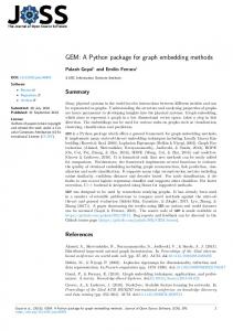
Fig. 1. Schematic view of a breaking pendulum variablebehavior model 2.1 Basics The basic idea of the approach in this paper is to use common simulation tools for the simulation and therefore use the power they already provide. It is not the idea to create a new language as was done by Zimmer (2010) with SOL or by Nilsson and Giorgidze (2010) with Hydra or with the tool MOSILAB (2011); Nordwig (2003) (these languages and tools will be discussed in section 4). The idea of our approach is to use scripts which handle the mode switches during simulation. To accomplish this each mode of a model needs to be an independent model which consists of variables and equations. Each of these modes has a stop condition which stops the simulation of this particular mode. Figure 1 shows a schematic view of a breaking pendulum model with two modes. One mode which is the normal pendulum and one mode which is a falling mass. To get from one mode to the next a script is used. The workflow is shown in figure 4. This script compiles all Dymola models and initializes and starts the first mode. As soon as the simulation is stopped the script takes control and calculates the startvalues for the next mode. The realization of the mode switches with Dymola is presented in the next subsection. The general approach was presented in Mehlhase (2011) where it was tested with Simulink models and Matlab-scriptss and with Dymola models with a MOS- and Matlab-scripts. The problem that still remained was that the MOS-scripts are rather slow in calculating new initial values and that Dymola can only store one compiled model. Therefore, for each mode switch a new compilation is necessary. The Matlab scripts with Dymola did work well and the problem with the many compilations can be overcome but two commercial tools are not feasible for a company. Furthermore, the scritping was only testes for two modes which each had one transtion. In this paper a Python package is presented which is faster and easier to handle for variable-structure models than Matlab. The package can also handle more than two modes and no expensive commercial tool is necessary. 2.2 Design of the package The design of the package is an object-oriented approach and is shown schematically in figure 2. The first layer is the user interface. The package provides a graphical user interface and a Python template to specify variablestructure models. A Domain Specific Language (DSL) is planned but not implemented yet. All three possibilities do not require the user to know how to program Python. With

Fig. 2. Schematic view of the design of the Python package

Fig. 3. Class structure of a variable-structure model the information given by the user through one of the interfaces a ModelObject is created. This ModelObject holds all the needed information about the variable-structure model like the modes, the stoptime, and the solver, see figure 3. Each mode is an instance of a class called DymolaMode which inherit from the class Mode. The Mode class stores the transitions exiting from the mode, a name, a mode number and the variables to be observed. The necessary operations to initialize and simulate a mode in Dymola is stored in the DymolaMode class. A transition is also an object (class Transition) and stores the information to which mode the transition leads, what end values have to be read from the old mode, and how to set the initial values for the new mode. Through this implementation it is possible to create variable-structure models with an arbitrary number of modes and transitions between these modes. The ModelObject is handed to a method called switch.py which handles the switching procedure, see figure 4. At the beginning of this method all Dymola models are compiled and saved under different names. For each mode the initialization file ’dsin.txt’ is read which gives an initialization matrix. From the information in the transitions it in known which variables have to be initialized when a mode switch occurs. These variables are searched in the initialization matrix and the indices are saved, as to make the setting of the values faster during the simulation process. The method then enters a while-loop which only stops when the user defined stoptime is reached. In this while-loop the current mode (DymolaMode) is initialized and simulated. When the simulation stops the end-values of the simulation is read through the ’dsinfinal.txt’ file which holds the same data as the initialization file only for the end-values. The indices from the beginning of the method can now be used to read the needed end-values. If the stop time is not reached the current mode is changed to the new mode, the new mode is initialized and the whileloop is continued. After the simulation the observed data is stored into a file.

Fig. 5. Creating modes for variable-structure models

Fig. 4. Program flow of the switch.py method The chosen design of the package has many advantages. First of all the package could also be used for normal Dymola simulations because the dymola-class can be used on its own. Therefore, users who are familiar with Python can use the package to pre- and postprocess their data or optimize their models better than using the Modelica intern scripting language. Also the design gives the opportunity to extend the package and make it into a whole framework which can handle different tools such as OpenModelica or Simulink. The framework could then be used to create variable-structure models where each modes could be simulated in a different tool. Furthermore, it might also be interesting to store solver information directly in the mode so each mode can have its specific solver. All this can be easily done in the presented package. With the presented implementation we present new means of object-oriented modeling. This object-orientation is not based on equations but on the definition of a variablestructure model. 2.3 Creating variable-structure models Here we present the pendulum model as an example on how to use the Python package. First lets consider the Modelica models needed for a variable-structure model. The scripting approach was chosen because we wanted to be able to use existing models and to reuse the models afterwards again. The scripting allows us to use our old models on its own because they are valid Dymola models, but each model needs a stop condition to be used as a mode in a variable-structure model so the model needs to be altered. Dymola with its object-oriented modeling language Modelica Association (2010) helps us to keep our old models as they are and extend our needed modes from the old models. Figure 5 shows the pendulum model as a cross between Statecharts to show when a mode switch

occurs and a class diagram. The two models ”Pendulum” and ”Falling mass” represent the original models. The other models are extended models of the two and have the stop condition (here called terminate) added and a variable ”switch to” which specifies the mode that needs to be entered next. Here it can be seen, that the original models have not changed and can be used as before only the extended models now represent the modes in the variable-structure model. After the models for the modes are defined the Python package can be used to define the mode switches for the variable-structure model. In this paper we will only present the template because the graphical user interface is harder to explain without many screen shots. The template looks as follows: stop = 10 # stoptime model = [’PendelScript.mo’] # filename modell1 = ’pendel_struc’ # name first mode modell2 = ’ball_struc’ # name second mode models = [modell1, modell2] # list of modes sol = SOLVER # global definition solver init =[] # SWITCH MODE 1 - > MODE 2 out1 = [’x’,’y’,’der(x)’,’der(y)’] in2 = [’x’,’y’,’vx’,’vy’] init.append([1,2, out1, in2]) # SWITCH MODE2 - > MODE 1 out2 = [’x’,’der(phi)’] in1 = [’x’,’dphi’] init.append([2,1, out2, in1]) save([’x’,’y’],[’x’,’y’]) switch(stop,sol,model,models,init,save) For each model the name of the modelfile and the name of the modes have to be specified. These modes will later be compiled with Dymola. Afterwards the transitions have to be defined. A user defines a transition with the mode number where the transitions exits and the mode number where the transition enters. Furthermore, the variables to

read from the old mode (out1 and out2) and the variables that will be set in the new mode (in2 and in1) have to be specified. The variable ”save” is like an observer where the user can define which variables from each mode should be saved in a datamatrix after the simulation. The datamatrix is per default saved as MAT-File but the user can specify other output filetypes as well. All the information is then given to the switch method which creates the ModelObject and all the mode objects with their transitions. This template can be used to create models with an arbitrary number of modes. 3. EVALUATION In this section we present different variable-structure models. With these models it is shows how useful variablestructure models are. We then use an easy variablebehavior model to analyze the scalability of the Python package. At the end of this section requirements a model needs to fulfill to be used as a mode in a variable-structure model are discussed. 3.1 Variable-detail models To show that variable-detail models can save simulation time we look at a diesel combustion engine model, see figure 6. In this model the environment pressure changes every five seconds and thus the pressure of the manifold changes. When the pressure of the manifold and environment are almost the same the throttle and manifold are not necessary anymore and can be taken out. When the pressure changes again the model has to become more detailed again to simulate the dynamic pressure change in the manifold.

the Residual time is larger. This leads to the conclusion that variable-detail models can make a simulation faster. We also compared the results of the cylinder pressure and temperature and the difference was less then half a percent which shows that we were able to make the simulation faster without significant loss of accuracy. Table 1. Simulation time for the diesel combustion engine in seconds Stop time 20sec / 7 switches Simulation time Compilation time Residual time Total time

One detail Dymola 17

Variable detail Dymola/Matlab 7.3

Variable detail Dymola/Python 7.3

1*1.2= 1.2 1

2*1.2= 2.4 3.3

2*1.2= 2.4 2.3

19.2

13

12

3.2 Variable-behavior models As an easy variable-behavior model we present a bouncing ball model. Here the bouncing ball does not just change its velocity when it hits the floor but becomes a spring and damper system which means the ball is elastic and bounces differently depending on the damping constant. Figure 7 shows the bouncing ball results with different damping constants. Interesting is that the ball can never fall below the surface as happens if only a ”when” statement (without extra precautions) is used in Modelica. Furthermore, the center of the ball is not exactly where the radius (1m) is but a little below depending on the specified mass of the ball, this makes the model more realistic. 3

height (m)

2.5

2

1.5

1

0

0.5

1

1.5

2

2.5

3

3.5

time (sec)

Fig. 7. Simulation result of the bounging ball model

Fig. 6. Schematic view of a diesel combustion engine variable-detail model The measured simulation times can be seen in table 1. Here the simulation times of the model with only one level of detail and the simulation times of the variable-structure model with Matlab (only a script) and the Python package is presented. The model is always simulated for 20 seconds and has 7 mode switches. The Compilation time is the time needed to compile the Dymola models and the Residual time is the time the script needs for starting the simulation, setting initial values and so on. The variable-detail models are faster to simulate then the one level of detail model even though two compilations are necessary and

As a model with more than two transition we present a breaking pendulum model where the rope can get stuck on a nail. The model is simplified to make it easier to understand: • The pendulums suspension point is (0,0) • The nail position is x ≤ 0 and y < 0 (”nailPoint”) • The falling mass model is valid on the left of the nail The simplified model is shown in figure 8 (only a few important variables are shown in this view). We still have two modes but when the rope passes the angle where the nail is located the rope length changes and therefore the suspension point of the pendulum. We make a mode switch into the same model but change the model parameters. If the centrifugal force goes below zero the

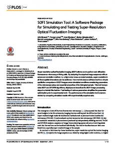
Fig. 8. Breaking pendulum model with nail pendulum becomes a falling mass otherwise it either turns around the nail or becomes the normal pendulum again. Figure 9 shows different movements of the pendulum for different start values of the angular velocity (dphi (rad/sec)) and the damping constant (D (N sec/m)). The normal suspension point and the nail are marked as dots. 1

dphi = −5, D = 0.04 dphi = −10, D = 0 dphi = −10, D = 0.1 dphi = −10, D = 0.09 dphi = −8, D = 0.2

0.5

y (m)

0

−0.5

−1

−1.5

−2 −2

−1.5

−1

−0.5

0

0.5

1

1.5

2

x (m)

Fig. 9. Simulation results of the breaking pendulum model with nail 3.3 Scalability of the simulations The scalability is always an issue with programs as presented here especially if one goal is to save simulation time. To test if the scripting approach with Python scales with the number of switches and the number of variables for initialization two different tests were made. For both test a bouncing ball model is used which has a transition to itself as soon as the ball touches the ground. Therefore, we have a ball that never stops bouncing. This model has only 2 statevariables (x,y) and these have to be initialized for each mode switch. As first test this model is simulated with 10, 100, 1000, 10000 mode switches, see table 2. It can be seen that the simulation time scales with the number of switches and it can also be seen where the most time is lost. The start of the dymosim.exe takes up a long time, but we do not have any means to change anything on the dymosim.exe routine. The other part that takes a long time is the reading of the end values of the old mode. In the implementation the dsinfinal.txt is changed into a Matlab file. This process does take up a long time and we are currently trying to find a better solution. The other measured times are the CPU time which is given by Dymola and is the time the simulation runs, the init time is the time it takes to set the initial values in the dsin file. This of course is a rather drastic example because the idea of variable-structure models is to use larger models with a long CPU time and a few switches and not a model with almost no CPU time and many switches.

As second example we use the same bouncing ball but this time we create an array with many of these balls. We always simulate for 10 switches but with 10, 100, 1000, and 10000 bouncing balls. This leads to many statevariables which have to be initialized. Now we see that the CPU time takes up most of the time, which was to be expected from larger models. We see that finding the inidces at the beginning of the simulation takes up a long time. There it can be seen that it is feasible to search the indices once at the beginning and not for each switch because the needed time would be even greater then. All other measured times are rather insignificant compared to the large CPU time for the large models. We see here that there is still some improvement necessary for the index search but otherwise the approach seems good for large models. 3.4 Modeling requirements After introducing the Python package,its design, and presenting examples of variable-structure models we are now discussing requirements for variable-structure models. Looking at the scalability test it is clear that it is not feasible to create variable-structure models with lots of mode switches especially if the models them self are really small. Many switches lead to an overhead in simulation time through the scripting. For variable-behavior models this might still be reasonable because one might otherwise not be able to simulate the system at all. Another problem with many mode switches is the initialization of the new mode. Each time a switch occurs an initialization problem has to be solved. If the values are chosen incorrectly or cannot be calculated from the old mode the numerical solution might become wrong or even instable. The initialization is therefore a great issue for variable-structure models and it is only possible to switch from one mode to the next if the new modes statevariables can be calculated through the variables of the old mode. This means not all models are fit to be used as modes in variable-structure models. For variable-detail models it is important that the models have a CPU time which is greater than the time the script consumes and also that the less detailed model at least compensates the scripting time otherwise no simulation time can be saved. Table 2. Simulation time for many switches in seconds Switches 10 100 1000 10000

overall time 0,64 5,21 55,34 544

index search 0,046 0,039 0,049 0,039

CPU 0,02 0,10 0,68 6,20

while-loop dymosim read 0,33 0,22 2,90 1,98 30,38 22,35 298,00 220,22

init 0,02 0,17 1,79 18,33

Table 3. Simulation time for large models in seconds Balls 10 100 1000 10000

overall time 5,00 6,75 14,93 322,27

index search 0,06 0,07 2,4 62,15

CPU 0,4 0,23 7,4 252,2

while- loop dymosim read 4,3 0,17 5,5 0,24 4,03 0,21 5,47 0,77

init 0,02 0,45 0,61 0,85

4. RELATED WORK

MOSILAB is a tool based on Modelica which can be used to model and simulate variable-structure models. This tool enhances the Modelica language and uses a Statecharts view to specify the mode switches, see Nytsch-Geusen et al. (2005). The drawback of MOSILAB is that it for now does only support index-0 models. The results we gather from this paper and our further research will be used to improve MOSILAB. The language SOL was developed by Zimmer (2010) and is an experimental Modelica like language. This language supports modeling variable-structure models, interpreting them and simulating them. An advantage of SOL is that when a mode switch occurs and the causalisation of the model changes only the necessary causalisations are made. This makes the mode switch quite elegant. SOL is an experimental language and thus far not available for large models, hopefully the results will sometime lead to a modeling language which supports variable-structure models. But a user cannot work with SOL right now and models from other tools would have to be specified in the new language. Another possibility for variable-structure models is Hydra which is described in Nilsson and Giorgidze (2010). Hydra is also a language under development which supports variable-structure modeling. It is based on functional programming languages and is therefore not as easy to learn for modelers. Keymaera from Platzer and Quesel (2008) is a verification tool for hybrid systems. Here hybrid systems can be modeled with hybrid automate and checked. All these possibilities have great ideas and do different things better than our approach but to model and simulation variable-structure models the user has to learn a new language and remodel their existing models. With our approach a common modeling tool can be used and Python is a free language which makes our approach accessible to anyone interested. Urquia and Dormido (2003) describe an algorithm which transforms a variable-structure model to a normal model by reformulating the modes into one mode. This approach does work but makes the resulting model quite large and will therefore extend the simulation time. This does not seem to be feasible for variable-detail models because simulation time will most likely not be saved. In Simulink it is possible to use enabled blocks to create a mode switch, but the definition of the transitions becomes rather complicated and the blocks that are disabled still take up simulation time, see Mehlhase (2011) for more information. In Dymola a mode switch is possible, as long as the variables do not change and the causality does not change. If either needs to change for a mode switch it is not easily possible. Elmqvist et al. (1993) describe a possibility for variablestructure models with if-statements in Modelica. Here the equations are reformulated, so depending on the mode the model is in, a multiplication with zero or one takes place. The equations therefore change during simulation. This approach does work but for large models with many mode switches it will become complicated. The equation system is also rather large and might slow down the simulation compared to a real mode switch.

5. CONCLUSION AND FUTURE WORK Our approach is not able to re-causalize only the needed equations or to have a just-in-time compiler as some other language and tools for variable-structure models have but we are able to use a common simulation tool for our simulation and therefore use the strength of this tool. We can use a tool like Dymola and give modelers the opportunity to test if variable-structure models are feasible for them. Our approach helps to easily create variable-structure models from existing models and use easy means to describe the models. We therefore hope that with our Python package knowledge of variable-structure models can be gained. In the future the package will be enhanced to a framework which will support different simulation tools. The framework should enable the user to use models from different tools as modes. With the planned framework researches are planned on what a tool needs to be usable for variable-structure modeling and when variable-structure models should be used to be feasible. REFERENCES R - A Unified ObjectAssociation, M. (2010). Modelica Oriented Language for Physical Systems Modeling Language Specification Version 3.2. Burmester, S., Giese, H., and Oberschelp, O. (2006). Hybrid uml components for the design of complex selfoptimizing mechatronic systems. In J. Braz, H. Arajo, A. Vieira, and B. Encarnacao (eds.), Informatics in Control, Automation and Robotics I. Springer Verlag. Dassault Systems (2011). URL www.dynasim.se. Elmqvist, H., Cellier, F.E., and Otter, M. (1993). Objectoriented modeling of hybrid systems. Mehlhase, A. (2011). Varying the level of detail during simulation. In ASIM 2011, Symposium Simulationstechnik. MOSILAB (2011). URL www.mosilab.org. Nilsson, H. and Giorgidze, G. (2010). Exploiting structural dynamism in Functional Hybrid Modelling for simulation of ideal diodes. In Proceedings of the 7th EUROSIM Congress on Modelling and Simulation. Czech Technical University Publishing House, Prague, Czech Republic. Nordwig, A. (2003). Integration von Sichten fr die objektorientierte Modellierung hybrider Systeme. Ph.D. thesis, Technischen Universitt Berlin. Nytsch-Geusen, C., Ernst, T., Nordwig, A., and et al. (2005). Mosilab: Development of a modelica based generic simulation tool supporting model structural dynamics. In G. Schmitz (ed.), Proceedings of the 4th International Modelica Conference, Hamburg, March 78, 2005, 527–535. TU Hamburg-Harburg. Platzer, A. and Quesel, J.D. (2008). Keymaera: A hybrid theorem prover for hybrid systems. In IJCAR. VOLUME 5195 OF LNCS, 171–178. Springer. R TheMathworks (2010). Simulink 7 User’s Guide (Release 2010b). Urquia, A. and Dormido, S. (2003). Object-oriented description of hybrid dynamic systems of variable structure. Simulation, 79(9), 485–493. Zimmer, D. (2010). Equation-Based Modeling of VariableStructure Systems. Ph.D. thesis, Swiss Federal Institute of Technology.