problem to the Minimal Vertex Cover in Graph Theory one. ..... König's theorem states that, in bipartite ... There are two possibilities for this: König theorem again ...
A Quadratic, Complete, and Minimal Consistency Diagnosis Process for Firewall ACLs S. Pozo, A.J. Varela-Vaca, R.M. Gasca QUIVIR Research Group, Department of Computer Languages and Systems Computer Engineering College, University of Seville Avda. Reina Mercedes S/N, 41012 Sevilla, Spain {sergiopozo, ajvarela, gasca}@us.es http://www.lsi.us.es/~quivir Abstract— Developing and managing firewall Access Control Lists (ACLs) are hard, time-consuming, and error-prone tasks for a variety of reasons. Complexity of networks is constantly increasing, as it is the size of firewall ACLs. Networks have different access control requirements which must be translated by a network administrator into firewall ACLs. During this task, inconsistent rules can be introduced in the ACL. Furthermore, each time a rule is modified (e.g. updated, corrected when a fault is found, etc.) a new inconsistency with other rules can be introduced. An inconsistent firewall ACL implies, in general, a design or development fault, and indicates that the firewall is accepting traffic that should be denied or vice versa. In this paper we propose a complete and minimal consistency diagnosis process which has worst-case quadratic time complexity with the number of rules in a set of inconsistent rules. There are other proposals of consistency diagnosis algorithms. However they have different problems which can prevent their use with big, real-life, ACLs: on the one hand, the minimal ones have exponential worst-case time complexity; on the other hand, the polynomial ones are not minimal. Keywords-inconsistency; conflict; anomaly; minimal; firewall; acl; ruleset; management; detection
I.
diagnosis;
INTRODUCTION
Although deployment of firewalls is an important step in the course of securing networks, the complexity of firewall ACL design might limit the effectiveness of firewall security. Writing and managing Access Control Lists (ACLs) are timeconsuming and error-prone tasks due to a variety of reasons [1, 9]. One of the main ones is that complexity of networks is constantly increasing, as changes in requirements, topology, etc. occur with higher frequency and density nowadays. According to Taylor [3], the number of rules in a firewall ACL usually ranges between a few ones and five thousand. Another reason is that networks have different access control requirements (or objectives) which must be translated by network administrators into firewall ACLs. The gap between the high-level access control requirements and low-level ACLs is too wide. Low-level firewall languages are difficult to learn, use and understand, and are very different from each other in syntax and semantics [27]. Although many high-level languages have been proposed in order to reduce design and development complexity and thus faults, no one have been widely adopted by the industry for various reasons [2]. Furthermore, their use does not guarantee that the resulting
ACL is fault-free, thus a method to diagnose design and development faults must be used in order to correct ACLs prior to its deployment. One of the most important and frequent faults during ACL design, development, and management are inconsistencies [1, 9]. A firewall ACL with inconsistent rules implies, in general, that the firewall is accepting traffic that should be denied or vice versa. This can cause severe problems such as unwanted accesses to services, denial of service, overflows, etc. ACL consistency is of extreme importance in several contexts, such as highly sensitive applications (e.g. health care). Since ACLs in complex networks are very big, giving the smallest set of rules that must be corrected is mandatory. Also note that when a rule is modified to correct an inconsistency, a new inconsistency with other rules can be introduced. Thus, the consistency diagnosis process should be run multiple times until no more faults remain. Furthermore, consistency management is becoming an important topic in a new range of applications for resource-constrained devices in ubiquitous networks such as ad-hoc network node real-time ACL updates, real-time IDS or IPS rule updates, QoS management, etc. For these reasons, the efficiency in time and space of the diagnosis process must be an important objective of the process. Many algorithms with these goals have been proposed earlier [5, 6, 10]. However, these proposals have many problems regarding different aspects of the diagnosis problem that prevent their use with big, real-life, ACLs. On the one hand, there are minimal proposals but with exponential worstcase time complexity. On the other hand, there are polynomial ones, but they are not minimal. In this paper, we propose a complete and minimal consistency diagnosis process for firewall ACLs with worstcase quadratic time complexity with the number of rules in a set of inconsistent rules. The union of these features is the main contribution of the paper. To the best of our knowledge, it is the first time that a process with these features has been proposed. Our proposal is based on a reformulation of the problem to the Minimal Vertex Cover in Graph Theory one. Experimental results with real ACLs that validate our proposal and compare it with other ones are also provided. The paper is structured as follows. In Section 2, consistency problems in firewall ACLs are explained and formalized. In Section 3 related works are reviewed. In Section 4 the minimal
diagnosis process is formalized and solved in quadratic time complexity. In Section 5 experimental results with real ACLs and a comparison with other proposals are provided. The paper finishes in Section 6 with some concluding remarks and insights for future works. II.
CONSISTENCY IN FIREWALL ACLS
As with other related works within the topic, this paper is focused in layer 3 firewalls, and thus in the five typical selectors [3]: protocol, source and destination IPs, and source and destination ports. Stateful and stateless firewall ACLs are supported, since there are no differences in their ACL formalization. A. Problem Formalization Firewall rule-matching engines match packets in a linear way, checking ACL rules from the first to the last one. The matching process stops once a rule has been matched, or once there are no more rules in the ACL (in this case, the firewall platform executes a predefined default action). The values of selectors (or filtering fields) between different rules can overlap, and can even be rules that are completely equal to others. An example of a layer-3 firewall ACL is presented in Fig. 1. A layer 3 Firewall ACL is a list of linearly ordered (total order) condition/action rules. Each firewall rule is formed by an antecedent and a binary consequent representing the action that must be taken once a packet matches the rule. Let PORTSRC and PORTDST be sets of natural numbers and intervals of naturals in [0..65535] representing port numbers. Let IPSRC and IPDST be two sets of valid IPv4 addresses in octet/CIDR format (o1.o2.o3.o4/CIDR). Let PROTOCOL be a set of natural numbers in [0..255] representing protocol numbers. Let ID≥1 be a natural number representing the rule priority in the ACL (1 is the rule with more priority). Let ACTION={Allow, Deny} be the binary set of possible actions for a rule. Let W=PROTOCOL×IPSRC×IPDST×PORTSRC×PORTDST be the cartesian product of the five previous sets or selectors, which represents a 5-dimensional hypercube. W is the space where an antecedent of a firewall rule can be defined. Definition 2.1. A firewall ACL or rule set, is defined as the cartesian product ACLf=W×ACTION, where |ACLf|=f. A rule in ACLf is defined as Rk ∈ ACL f ,1 ≤ k ≤ f , k ∈ ID . Rk[PROTOCOL], Rk[IPSRC], Rk[IPDST], Rk[PORTSRC], Priority/ID R1 R2 R3 R4 R5 R6 R7 R8 R9 R10 R11 R12
Protocol tcp tcp tcp tcp tcp tcp tcp tcp udp udp udp udp
Source IP 192.168.1.5/32 192.168.1.*/24 *.*.*.*/0 192.168.1.*/24 192.168.1.60/32 192.168.1.*/24 192.168.1.*/24 *.*.*.*/0 192.168.1.*/24 *.*.*.*/0 192.168.2.*/24 *.*.*.*/0
Rk[PORTDST], Rk[ACTION] represent the corresponding selectors of the rule Rk and its action. Example 2.1 (Rule). Take rule R1 in Fig. 1. In this case, following Definition 2.1: k=1, R1[PROTOCOL]=6, R1[IPDST]=0.0.0.0/0, R1[PORTSRC]=[0..65535], R1[PORTDST]=[80], R1[ACTION]=allow. Definition 2.2. ACLf can be trivially divided in two disjoint sets, one composed of rules with Allow action (ACLallow, where |ACLallow|=m), and the other composed of rules with Deny action (ACLdeny, where |ACLdeny|=n). Thus ACLallow ∪ ACLdeny = ACL f and ACLallow ∩ ACLdeny = ∅ Example 2.2. Take Fig. 1 example, where ACLallow={R2, R3, R6, R7, R9, R10, R11} and ACLdeny={R1, R4, R5, R8, R12}, then ACLallow ∩ ACLdeny = ∅ . Definition 2.3. Let the antecedent of a rule of Rk ∈ ACL f
be defined as an element or subset of W, a ( Rk ) ⊆ W . Let the consequent of a rule Rk ∈ ACL f be defined as
c( Rk ) ⊂ ACTION . The union of the antecedents of all rules in m
ACLallow is the set A, A = ∪a( Ri ∈ ACLallow ) / c( Ri ) = allow . 1
The union of the antecedents of all rules in ACLdeny is the set D, n
D = ∪a( R j ∈ ACLdeny ) / c( R j ) = deny 1
Definition 2.4. Ri and Rj are mutually inconsistent, I(Ri, Rj) ├ ⊥ ⇔ a( Ri ∈ ACLallow ) ∩ a( R j ∈ ACLdeny ) ≠ ∅ . Two elements in ACLf representing an action and the contrary over a subset of W are logically inconsistent. In the same way ACLf is inconsistent ⇔ A ∩ D ≠ ∅ . Consistency is not affected by the relative priority between rules. An inconsistency is considered to be a fault if an administrator identifies the behaviour of the executed ACL as being causing undesirable effects (or having errors). Example 2.4. Take Fig. 1 example. R1 and R2 are inconsistent (there are more inconsistencies in this ACL). Fig. 1 ACL is also inconsistent, since there is at least one pair of inconsistent rules, and thus A ∩ D ≠ ∅ . Definition 2.5. Inconsistency Isolation. It is the action of Src Port * * * * * * * * * * * *
Destination IP *.*.*.*/0 *.*.*.*/0 172.0.1.10/32 172.0.1.10/32 *.*.*.*/0 *.*.*.*/0 172.0.1.10/32 *.*.*.*/0 172.0.1.10/32 172.0.1.10/32 172.0.2.*/24 *.*.*.*/0
Figure 1. Example of a layer-3 Firewall ACL
Dst Port 80 80 80 80 21 21 21 any 53 53 any any
Action deny allow allow deny deny allow allow deny allow allow allow deny
finding out all Ri ∈ ACLallow , R j ∈ ACLdeny such that I(Ri, Rj) ├ ⊥. The isolation process identifies all the inconsistent rules of ACLf. The set of the isolated rules is INC. Definition 2.6. Minimal Diagnosis Set. The Minimal Diagnosis Set MDS ⊆ INC is a set such that ACL f − MDS is consistent. Therefore if all rules in MDS are removed or corrected and no more inconsistencies are introduced, ACLf ├T. MDS is minimal iff there is no proper subset of INC, MDS ' ⊂ INC , such that | MDS ' | < | MDS | , with MDS’ being a diagnosis.
B. Example An example of a layer-3 firewall ACL is presented in Fig. 1. Note that this example ACL can represent both stateful and stateless firewalls, since they do not differ in the number or type of selectors. In this example, R 4 ⊂ R 3 because all selectors of R4 are at least subsets of the same selectors of R3. However, their actions are the opposite. In this case R4 is never going to be matched in this ACL, because all packets that R4 could match are also matched by a rule with higher priority, R3. In this case, the firewall administrator must be notified, since R3 may be a faulty rule (the consequence, or the error, is that there is traffic that is allowed by R3 and it may be denied). Take as another example the rules R1 ⊂ R 2 . In this case traffic that is denied by R1 is also accepted by R2. This kind of relation is used by administrators to express exceptions (the most specific rule, R1) to a general rule (R2), and is not usually considered to be a fault, because there is no error in the ACL execution. Note that in the examples, actions are always different. If actions were equal, there is no potential erroneous behavior in the executed ACL, and thus there is no inconsistency. However there is redundancy, which is another kind of fault which can reduce the performance and increase the memory consumption of the rule-matching engine. In this paper, we only consider rules which can be potential faults, or inconsistent rules.
C. Consistency Management Cycle In earlier works [16] we proposed to divide the ACL consistency diagnosis problem in three automatic sequential steps: inconsistency detection and isolation, minimal identification of the rules to be corrected (minimal diagnosis), and the characterization of the diagnosis. In this paper, we augment that automatic process in order to define the Consistency Management Cycle, CMC (Fig. 2). Although we have made contributions in all parts of the cycle in the past, this
paper is focused in the fourth step, Minimal Identification of Inconsistent Rules. However, to give context to the reader, all parts of the cycle are briefly described below. In the proposed CMC, the ACL must be first designed and developed by an administrator. There are several alternatives for this part of the process: high-level languages [2], low-level languages, commercial or free tools based on GUIs, etc. Next, redundancies should be automatically detected and corrected. The objective is twofold. On the one hand, an ACL without redundancies is smaller than an ACL with them, and thus reduces the time and memory required to process packets when the ACL is deployed. On the other hand, redundant rules can cause more inconsistencies that do not give the administrator important information, since they are redundant inconsistencies. As we described earlier in this section, redundancies are not a consistency problem, because they do not change the semantics of the ACL. Redundancies can be detected and removed in quadratic time using automatic algorithms as the proposed by Liu et al. [25]. In the third one, inconsistent rules must be detected and, if any, isolated from the ACL. This third step of the process is important in order to know if a rule of the ACL is inconsistent with others, if a modification of a rule can cause new inconsistencies, or even to know if a new rule being introduced in the ACL could cause inconsistencies with the existing ones. However note that in Fig. 1 example all rules are mutually inconsistent with at least another rule in the ACL, and thus all of them will be isolated in this step of the CMC process. Thus another step (the fourth one) is necessary in order to compute (identify) which of the isolated inconsistent rules are the ones that, once corrected or removed, make the ACL consistent. This result must be complete, i.e. with the identified rules it must be possible to correct all inconsistencies in the ACL. Since the Parsimony Principle says that the preference for a diagnosis of a problem is to give the least complex explanation, the optimal result for the identification step is the minimal one. This is especially important for big ACLs and in ACLs with a lot of inconsistencies, since not giving it could result in an overwhelming number of rules to be corrected. The result of the identification part of the process can be used to automatically correct the ACL using schemas such as the one proposed in [6]. Both third and fourth steps of the CMC are the consistency diagnosis of the ACL, because with this result it is possible to correct all inconsistencies. Several algorithms with different complexities can be used to give a minimal diagnosis [5, 6, 15]. However, these algorithms have exponential worst case time
Figure 2. Concistency Management Cycle, CMC
and space complexity, which prevents their use with big, reallife ACLs. To the best of our knowledge, it has been proposed no polynomial algorithm to solve the minimal diagnosis problem, but only heuristics [26]. In earlier works, we proposed a worst case quadratic firewall-ACL-specific algorithm for step three (inconsistency detection and isolation) [16]. The main objectives and contributions of this work are the demonstration of that a quadratic space and time minimal and complete identification (fourth part of the CMP) algorithm exist and a proposal of one. The fifth step of the process is the diagnosis characterization. Note that with the result of the diagnosis, an experienced administrator has to check the diagnosed rules in order to know which kind of inconsistencies are faults or not. Recall from the first part of this section that there could be inconsistencies that do not generate an erroneous behaviour in the ACL. However, there exist a well accepted and established taxonomy of consistency faults for firewall ACLs, which has been formally proved to be complete [14]. Thus, even more accurate results can be given to the administrator if the diagnosis is characterized using this taxonomy. Finally, once the inconsistencies have been characterized, the administrator must correct them or not, depending if they cause errors or not. Note that once inconsistencies have been corrected, there is no guarantee that the new inconsistencies or redundancies are introduced. Thus, the full consistency management cycle starts again until the desired ACL is obtained. This is one of the reasons why the performance of the CMC is a key part of the problem. III.
RELATED WORKS
There are mainly two research lines focused in diagnosis algorithms for firewall ACLs. In the first one, the proposals are focused in firewall ACLs, characterizing the diagnosis using a known and complete fault taxonomy [14]. In some of these works the given diagnosis is minimal, but the results are usually given in exponential time complexity. In the second one, the proposals are more general, and are not focused in firewall ACLs, but in network filters in general. These works do not give a minimal diagnosis, and neither characterize it, although their complexity is polynomial. The most important works in the first research line (minimal diagnosis and its characterization) were made by AlShaer et al [5]. In their works, authors’ define a complete inconsistency taxonomy for firewall ACLs [14] which include redundancies. They provide a rule order-dependent consistency diagnosis algorithm between every pair of rules in the ACL. An indivisible part of their diagnosis algorithm is the characterization of the faults found, using their own taxonomy, which has been formally proved to be complete [14]. However, one of the main drawbacks of this proposal is that the algorithms do not characterize inconsistencies with a combination of more than two rules and thus the diagnosis could not be minimal. In fact, the result given by this proposal is an isolation of inconsistent pairs of rules (Definition 2.5, previous section), and not a diagnosis. In the worst case (i.e. all rules are inconsistent in an ACL), the number of returned pairs of inconsistencies could be ACLallow·ACLdeny.
Another important drawback of this proposal is that they use an ACL decomposition technique in order to make the problem tractable for big ACLs. This technique is called rule decorrelation [8]. The result of this decomposition is a new ACL with no overlapping rules. This new ACL is the real input for their diagnosis algorithms. However, as the decorrelated ACL is free from rule overlaps, it could have more rules than the original one, and so the problem size is bigger than the size of the original ACL. Furthermore, the decorrelation process used [8] is worst-case exponential time and space complexity with the number of decorrelated rules. Although the diagnosis and characterization algorithms proposed by Al-Shaer are worst-case polynomial, the decorrelation pre-process dominates the complexity of the full process. Finally, results are given over the decorrelated ACL, but the firewall administrator must correct faults over original ACL without any aid to reverse the decorrelation. A modification to Al-Shaer proposal was provided by García-Alfaro et al [6], where they integrated the decorrelation, consistency diagnosis, and characterization algorithms (including redundancy) of Al-Shaer, proposal plus an automatic ACL correction, in only one step. One of the improvements of García-Alfaro proposal is that they provide a characterization technique with multiple rules, instead of the pair-wise one of Al-Shaer. However, due to the use of the same decorrelation techniques, García-Alfaro’s proposal has the same drawbacks of Al-Shaer’s one, including the exponential time complexity. In Fireman [15], authors’ have addressed the consistency diagnosis and characterization problem using a formal model of the firewall ACL. They solved the problem using Ordered Binary Decision Diagrams (OBDDs), providing the first technique which does not need to decompose the ACL. As with García-Alfaro’s proposal, this technique is also able to give inconsistencies and redundancies within several rules, and not only between pairs. Authors provide an experimental analysis in which it can be seen that the time complexity is linear with the number of rules in the ACL. However, the minimal diagnosis is not guaranteed. In order to guarantee it, OBDD nodes must be optimally ordered, but the optimal node ordering of OBDDs is a NP-Complete problem [19]. The bottom line is that Fireman is the best proposal to date, but if a minimal diagnosis is desired, the process is worst-case exponential time complexity. In the second research line, Baboescu et al. [10] provide diagnosis algorithms that are 30 times faster than the trivial quadratic one for the general case of k selectors per rule and for general network filters. In fact, they provide two different diagnosis algorithms: one for the diagnosis of a full ACL, and another one for ACL management (only used when the ACL has been developed). The reason is that their proposal has a trade off between the space needed and speed in the diagnosis algorithm. The minimal diagnosis is not guaranteed in neither of the two algorithms, since it depends on the topology of the abstract data types they use (bit tries). Furthermore, Baboescu definition of inconsistency is more general than Al-Shaer taxonomy ones, and does not include redundancies. Babouescu technique is also able to give inconsistencies within several rules.
Although its algorithmic complexity is not given, it empirically improves other previous diagnosis proposals made by Hari et al and Suri et al [11, 12]. Like Al-Shaer and GarcíaAlfaro proposals, Baboescu algorithms depart from a decomposed ACL, where selectors that support intervals have been converted to binary prefixes using the range to prefix conversion technique [7]. This technique splits the selectors which contain ranges into several prefixes and thus the final number of rules could increase over the original ACL. Taylor [3] and Gupta [13] outlined that this kind of conversion could be inefficient, because transport layer specifications vary widely (for example it is possible to specify open port ranges, such as “all ports greater than 1023”). Taylor also calculated that, in the worst case, a range covering w-bit port numbers may require 2(w-1) prefixes, and that a single ACL including only two port ranges could require 2(w-1)2 entries (i.e. 900 entries for 16-bit port numbers), increasing the number of rules in the ACL and the problem size. Fortunately, the decomposed ACL could be trivially reverted to the original one in order to correct faults more easily. With real ACLs, the time complexity of the diagnosis algorithms entirely depends on the increase in the ACL size derived from the use of the range to prefix decomposition. If the ACL size does not increase very much, Baboescu’s algorithms are really fast; but if the ACL size increases a lot, it could be even more inefficient than the trivial algorithm (comparing every pair of rules of the original ACL in quadratic time), as is going to be shown in the experimental results section of this paper. There are several important differences between our work and the reviewed ones. The most important one is that our process is divided in two sequential parts, which use different kind of techniques to be solved. In the first part, inconsistent rules are isolated using a technique which does not need to decompose the ACL and with has better time complexity than Baboescu’s proposal. This technique is also able to give inconsistencies within several rules. This first part of the process is not covered in this paper, since it has been proposed in an earlier work [16]. With Baboescu’s proposal it is also possible to obtain a similar result, but with higher time complexity. The result of this first part of the process is a complete but non-minimal set of inconsistent rules (INC, Definition 2.5), and is the input to the process provided in this paper. In this paper we propose a process to get a minimal diagnosis in worst-case quadratic time complexity with the number of rules in INC. In order to get this result, we formally prove that the problem can be reformulated to a known graph one, the Minimal Vertex Cover [22], which can be solved in quadratic time. Note that in
Figure 3. IG derived from Fig. 1 example ACL
our proposal, redundancies are not considered. To the best of our knowledge, this is the first time that a non exponential process to minimally solve the diagnosis problem in firewall ACLs has been formally proved to be possible, and algorithms provided. IV.
MINIMAL CONSISTENCY DIAGNOSIS
The start point to the minimal diagnosis process is the transformation of the INC set into a graph called Inconsistency Graph, IG (Definition 3.1). The graph can also be constructed during the execution of the inconsistency isolation algorithm, during the step three of the CMC. Definition 3.1. Inconsistency Graph. An IG(V,E) is a graph whose vertices are the rules in INC (i.e. the inconsistent rules of ACLf), and whose edges are the inconsistency relations between these rules. Note that |V| is the number of inconsistent rules in ACLf, and |E| corresponds with the number of inconsistencies in ACLf.
The IG has been proposed in an earlier paper [20]. However, in this paper we provide an analysis of its properties which are the key to obtain a minimal diagnosis in quadratic time reformulating the problem to a Graph Theory dual one: • Property 1. IG is not directed. Given two rules, Ri ∈ ACLallow and R j ∈ ACLdeny , if they are inconsistent, the inconsistency is, by Definition 2.4, mutual. Since edges in the IG represent inconsistencies, they must not be directed. • Property 2. IG is bipartite. Let assume the action of the rules in the IG as a colour. Then, the vertices in the IG can be divided in two disjoint sets, each one storing rules of one of the two colours: U for allow-coloured rules, and V for deny-coloured rules. As rules can only be inconsistent if they have different actions (by Definition 2.4), edges in the IG must always be between vertices of different colours (i.e. every edge in the IG connects a vertex in U to one in V, and there can never be edges between vertices in U or between vertices in V). The IG is thus 2-colorable. A graph is bipartite iff it is 2-colorable [22]. Thus the IG can be redefined as IG(U,V,E). In graph theory, U and V are called Independent Sets. The IG of the example ACL (Fig. 1) is presented in Fig. 3. Light gray-coloured vertices represent rules with allow action, and dark grey-coloured vertices represent rules with deny action. • Property 3. IG could have more than one connected component. In an ACL there could be cases where the same inconsistency is shared between several rules. For example, in Fig. 3, R12 is inconsistent with rules R9, R10, and R11. This happens when the rules with the same action have overlapping selectors. There could also be cases where inconsistencies are only between pairs of rules. Each set of inconsistencies with rules not related with others in the ACL leads to different connected components in the IG. In Fig. 3 there are two connected components: one with rules C1={R1, R2, R3, R4, R5, R6, R7, R8}, and the other with rules C2={R9, R10, R11, R12}. Rules in C1 do not overlap
MDSMVC. A MVC is a minimal set of vertices such that every edge of a graph is incident to at least one vertex in the MVC. Thus, if all the vertices in the MVC are removed from the graph, the resulting one contains no edges. Figure 4. Resulting IG with MDS1 vertices removed: the IG (and thus ACLf) are consistent
with rules in C2, and thus a rule in C1 can never participate in an inconsistency with a rule in C2. The maximum number of connected components in the IG is theoretically limited by the maximum number of inconsistencies in the corresponding ACL (or edges in the IG). • Property 4. |Emax|=|U|·|V|. In a bipartite graph, the maximum number of edges is U·V [22]. This is an important property because it can be used to measure the IG maximum density. Although there is no agreed definition of how to characterize a dense or sparse graph (i.e. which is the cut value in the number of edges to consider a graph dense or sparse), one of the most accepted characterization for undirected graphs have been given by Coleman and Moré [21]. They define a dense graph as a one which its number of edges, |E|, is near the maximum possible, U·V. The maximum density could be used to know if IGs used in the experimental analysis have a high number of inconsistencies or not, with respect to the maximum possible, ACLallow·ACLdeny.
From the previous section, recall that the objective of the minimal diagnosis is to compute which, from the isolated rules, are the minimal ones that once corrected or removed make the ACL consistent (Definition 2.6, Minimal Diagnosis Set). It is implicit that the MDS is also complete. However, there could be more than one MDS. This is the case of the example presented in Fig. 1 (IG of Fig. 3), where there are two and minimums: MDS1={R1,R4,R5,R8,R12} MDS2={R2,R3,R5,R8,R12}. In this paper, and in absence of specific criteria, we assume that any minimum is valid (e.g. the first found). Fig. 4 presents the resulting example IG when MDS1 vertices (and their corresponding edges) have been removed. In the next section we explain how to obtain one of the possible MDS in quadratic time. A. Problem reformulation During the reformulation of the problem to graph theory, we found that a dual one is the Minimum Vertex Cover (MVC). A vertex cover [22] of a graph G is a set of vertices C such that each edge of G is incident to at least one vertex in C. The set C is said to cover the edges of G. A minimum vertex cover is a vertex covering of the smallest possible size [22]. However, a demonstration is needed in order to assure this duality and generalize the result to any IG. MDS MVC. A MDS is a minimal set of vertices such that if they are removed from the IG, the resulting one contains no edges (and thus the corresponding ACLf is also consistent). Therefore, each edge of the IG is incident to at least one vertex in the MDS.
MDS MVC. Since the objective functions to be optimized in both MDS and MVC problems are the same, and is the minimum number of vertices (rules) which if removed (or corrected) make the IG (or ACLf) consistent, solving the MDS and MVC problems over the same IG give equivalent results.
B. MVC Problem and Algorithms Finding a MVC is a classical optimization problem in computer science and also a typical example of an NP-hard optimization problem. However, for some graphs with special characteristics the problem can be solved in polynomial time. This is the case of bipartite graphs, like the IG. Moreover, the MVC problem can be formulated as a half-integral linear program whose dual linear program is the Maximum Matching Problem (MM) [22]. In graph theory, a Matching or EdgeIndependent Set of a graph is a set of edges without common vertices. This is a very important duality, since there are no known algorithms to directly solve the MVC problem in bipartite graphs in polynomial time. However, there exist many algorithms that can solve the MM problem in bipartite graphs in worst-case quadratic time and space [22] with the number of vertices and edges in the graph, and which can be directly applied to an IG. This is the case of Hopcroft-Karp [23] or Alt [18] algorithms. However, with all these algorithms the Maximum Matching (a set of edges) must be converted to a MVC. Fortunately, this can be done in quadratic time via König’s theorem [22]. König's theorem states that, in bipartite graphs, the MM is equal in size to the MVC. Although there are many other algorithms, the objective of the paper is not to explain them, because there are very good descriptions (and also implementations) available in the bibliography. Nevertheless, there is more general way of getting a MVC: using algorithms to solve the Maximum Flow problem in flow networks. A flow network is a directed graph where every edge has a capacity and where each edge receives a flow. The amount of flow on an edge cannot exceed its capacity. A flow must satisfy the constraint that the amount of flow into a vertex equals the amount of flow out of it. However, source vertices only have outgoing flow, and end vertices or (sinks) only have incoming flow. The maximum flow problem is to find a feasible maximum flow through a single-source, single-sink flow network. Fortunately, undirected bipartite graphs can be reduced to a flow network, where fictitious source (super-source) and sink (super-sink) vertices are added to the graph. Undirected edges are transformed to directed ones from the source node to the sink. All edges have a capacity of 1. Ford-Fukerson [24], Edmonds-Karp [4], and Dinic [17] algorithms use basically the same technique (augmenting paths [22]) and can be used with a similar time bound in bipartite graphs, worst-case O((|U|+|V|)·|E|). Ford-Fulkerson and Edmonds-Karp algorithms are the most used, because they have the lowest multiplicative constant in the time bounds and the smallest space complexity.
ssrc
component. In this case, different flows can pass through each one without affecting other components’ flows. However note
ssrc
R2
R3
R6
R7
R1
R4
R5
R8
R9
R10
R11
Figure 6. Result of the Minimal Consistency Diagnosis of Fig. 1 ACL R12
ssink
ssink
MIN-CUT EDGES (PARTITION 1)
MIN-CUT EDGES (PARTITION 2)
{R1, ssink},{R4, ssink},{R5, ssink},{R8, ssink}
{R12, ssink}
MINIMUM VERTEX COVER (PARTITION 1)
MINIMUM VERTEX COVER (PARTITION 2)
{R1, R4, R5, R8}
{R12} MINIMUM VERTEX COVER (FULL GRAPH) {R1, R4, R5, R8, R12}
Figure 5. Flow network, min-cut, and MVC derived from Fig. 2 example IG (one the two possible minimum solutions, MDS2)
As with algorithms for the Maximum Matching Problem, the maximum flow result (edges) must be transformed to vertices. There are two possibilities for this: König theorem again, or the more direct Max-flow Min-cut theorem. Maxflow Min-cut theorem [22] states that in a flow network, the maximum amount of flow passing from the source to the sink nodes is equal to the minimum capacity that needs to be removed from the network so that no flow can pass from the source to the sink. In other words, the maximum value of a flow from the source to the sink is equal to the minimum capacity of a source-sink cut. In graph theory, a cut is a partition of the graph vertices into two disjoint subsets. In a flow network, a source-sink cut is a cut that requires the source and the sink to be in different subsets. A cut is minimum if the size of the cut is not larger than the size of any other cut. In fact, the same algorithms used to calculate the max-flow can also be directly used for the min-cut in bipartite graphs, giving a direct Minimal Vertex Cover result. One question that may arise is how to deal with rule updates, since running the whole process each time is not an effective way of doing it. This topic has been covered in earlier works [28]. C. Example By Property 3, an IG can have more than one connected TABLE I. ACL Size 50 144 238 450 900 2500 5000 10611
No. of Deny rules, |U| 11 34 95 116 116 163 97 213
No. of Allow rules, |V| 39 110 143 334 784 2337 4903 10398
that different source and sink nodes are necessary for each component. A beneficial lateral effect of this property is that the maximum-flow and min-cut algorithms can be run in parallel for each component. Property 3 thus allows a reduction of the problem by a factor that depends on the number of connected components in the graph. We will illustrate this in the experimental results section. The MVC for the full graph is computed by the union of the MVCs of each connected component. Fig. 5 shows the two flow networks resulting from the decomposition of Fig. 3 example IG, the min-cut edges in each component, and the resulting MVC. Note that this example only represents one of the two possible minimums, MDS2. Since the MVC is equivalent to the MDS in an IG, this is the desired result, which has been obtained in worst case O((|U|+|V|)·|E|) time and space complexity with the number of vertices and edges in the IG. Recall that MDS vertices directly correspond to vertices in ACLf, which is the original ACL that was developed by the firewall administrator. Moreover, more information could be given to the administrator: the MDS plus the rules which they are inconsistent with (Fig. 6), resulting in a diagnosis with multiple rules, in contrast with other pair-wise diagnosis techniques. This information can be trivially obtained from the IG by getting the adjacent vertices to the MDS ones in the original IG. Although our process does not include a diagnosis characterization step, it can be trivially added applying AlShaer’s taxonomy [14]. V.
EXPERIMENTAL RESULTS
In absence of standard ACLs for testing, experimental results have been obtained using real firewall ACLs. These ACLs represent a wide spectrum of cases, with sizes ranging from 50 to 10611 rules, and percentages of allow and deny rules from 2% to 65%. Table I presents the characteristics of these ACLs as well as its associated IG characteristics. The first column represents the size of the ACL; the second and third ones the number of a deny and allow rules; the fourth one the theoretical maximum number of edges (inconsistencies) that the IG could have, |U|·|V|; the fifth one the real number of
EXPERIMENTAL ACL AND IG CHARACTERISTICS
Theoretical |E|max in IG 429 3740 13585 38744 90944 380931 475591 2214774
Real |E| in IG 37 108 231 422 871 3349 4937 11866
|U|+|V| in IG 39 110 149 340 789 2399 4909 10488
Connected Components 2 2 2 2 2 2 1 1
Component 1 size 19 47 92 190 374 978 4909 10488
Component 2 size 20 63 57 150 415 1421 -
Although algorithms can run in parallel, our implementation is sequential.
Figure 7. Theoretical number of edges in IG vs real edges
edges in each IG; the sixth one the number of vertices in the IG for each ACL; the seventh one, the number of connected components; and the two final columns, the number of vertices in each one. Experiments were performed on a mono-threaded Java implementation with Sun JDK 1.6.0 64-bit HotSpot VM on an isolated HP Proliant 145-G2 server (AMD Opteron 275 2.2GHz, 2Gb RAM DDR400). Note that, in general, the analyzed ACLs result in sparse IGs, i.e. graphs where the number of edges (inconsistencies) is not near to the maximum possible (Fig. 7). This is very important, since the computational complexity of all the algorithms for the Maximum Flow and Maximum Matching problems depend on the number of edges in the graph. In fact, this was a very predictable thing, since other experimental analysis made in the past have confirmed [5, 1] that, in general, the number firewall ACL inconsistencies is very low compared to the theoretical maximum. Also note that the maximum number of connected components for the test ACLs is very low, with only one or two components. When there is more than one component, sizes are more or less equilibrated, which is the best possible case. Recall from the previous section that is necessary to run a different maximum flow algorithm for each component. TABLE II. ACL Size
|MDS|=|MVC|
50 144 238 450 900 2500 5000 10611
2 2 10 10 10 32 6 41
50 144 238 450 900 2500 5000 10611
Trivial algorithm Diagnosis Set size 37 108 231 422 871 3349 4937 11866
Results show that the identification of inconsistent rules part of the process is linear, with a very low multiplicative constant [16]. The graph construction time takes approximately half the time needed to identify these inconsistencies, which also gives and idea of how low the complexity of the identification part of the process is. The minimal diagnosis, in the other hand, has a very high execution time when compared with the previous part of the process. However, in all cases the time needed is under 2000ms. In fact, the time needed for the whole process is always below 2000ms. We think that these times are very reasonable even for really big ACLs, especially when taking into account that the full process must be run iteratively until all faulty rules have been corrected or removed. However, if the minimal diagnosis is not desired, the execution times are very low (Table II, third column). Table III represents the evaluation of other algorithms in order to have an idea of the improvement obtained with our proposal. Note that in this table only the trivial and Baboescu proposals have been evaluated. The reason is that they are the closest ones to ours, although neither of them gives a minimal diagnosis. Al-Shaer’s, García-Alfaro’s, and Fireman proposals have been left out of the evaluation because they include
EVALUATION OF OUR PROPOSAL
Inconsistent rules IG construction (ms) Identification (ms) 0.11 0.03 0.23 0.10 0.39 0.23 0.80 0.42 1.54 0.86 4.40 3.71 10.08 6.05 30.16 17.89 TABLE III.
ACL Size
Table II presents the results of the experiments with our proposed scheme. For the Minimal Vertex Cover we have chosen Edmonds-Karp algorithm. First column represents the ACL size; the second one the size of the minimal diagnosis set; the third one the time taken by the inconsistency isolation algorithm used [16] (including ADT instantiation time); the fourth one the time needed to build each IG; the fifth column represents the execution of the process proposed in the paper, that comprehends the division in connected components of the graph, the conversion to flow networks of each component, the Edmonds-Karp algorithm for each one, the conversion of the results to the MVC, and the union of the results for each component (where applicable); finally, the last column represents the total time needed to get a minimal and complete consistency diagnosis using our proposal.
Trivial algorithm execution (ms) 0.22 1.34 3.56 13.22 51.57 387.86 3160.09 12046.67
Minimal Diagnosis (ms) (Edmonds-Karp) 0.32 0.96 2.16 4.33 11.30 148.53 150.80 1919.48
TOTAL (ms) 0.47 1.29 2.78 5.55 13.70 156.64 166.93 1967.53
OTHER PROPOSALS EVALUATION
Baboescu algorithm decorrelated ACL size 203 21970 52129 52765 53219 69559 733547 877582
Baboescu algorithm Baboescu algorithm increase of ACL size Diagnosis Set size 4.06 2 360.9 2 219.03 14 117.26 14 59.13 14 27.82 70 146.71 10 82.7 103
Baboescu algorithm execution (ms) 9.96 270.41 381.55 461.17 626.69 2614.17 22062.10 91263.17
Figure 9. Execution time of different proposals Figure 8. Theoretical number of edges in IG vs real edges
redundancy diagnosis and a diagnosis characterization stage, and these parts are inseparable of consistency diagnosis in their algorithms. The first column represents the ACL size; the second and third ones represent the size of the Diagnosis Set given by the trivial algorithm (the same one as |E| in their corresponding IG) and its execution time, respectively; the fourth and fifth columns are the size of the ACL once it has been decomposed by the range to prefix technique (this is the input to the Baboescu algorithm), and the increase in size over the original one; the sixth column represents the size of the Diagnosis Set given by Baboescu algorithm; finally, the seventh column is the time taken by the Baboescu diagnosis algorithm, including ADT instantiation (bit tries). The first thing that should be noted is the really low cardinality of the MDS (Table II, second column, and Fig. 8). Even for really big ACLs, the number of inconsistent rules that must be corrected or removed is under 45, which contrasts with the high number of inconsistencies returned by the trivial algorithm (Table III, second column). This clearly shows that giving the smallest possible diagnosis is a must in order to reduce the number of rules given to the firewall administrator. Even with the Baboescu algorithm (the best one to date) the size of the Diagnosis Set doubles the size of the minimal one, although for small ACLs the Diagnosis Set is of the same size as the minimal one. Execution time of the trivial algorithm (Fig. 9) is only faster than the total time taken by our process in the ACL of size 50, even with the fact that in our proposal there is a start-up time needed to create some ADTs [16]. However, this was predictable, since the theoretical complexity of our proposal is, in the worst case, an order of magnitude faster than the trivial one. This contrasts a lot with Baboescu’s proposal, since their execution time is even slower than the trivial one and, in their paper they state that their proposal is about 30 times faster than the trivial one. Fortunately, there is a clear and simple explanation for this: the problem size increase due to the range to prefix decomposition could be very inefficient, as has also been stated by Taylor [3] and Gupta [13]. This is represented in Table III, fourth and fifth columns, with an average increase size of 127.20 times for the test ACLs. Thus, Baboescu proposal is only faster than the trivial one for big ACLs and when the increase in size is not too much (about 10 to 15 times).
VI.
CONCLUSIONS AND FUTURE WORKS
In this paper we have proposed a quadratic time and space complexity process for the Minimal Consistency Diagnosis problem in firewall ACLs. For this, the problem has been transformed to a graph, and its properties analyzed. Then we have demonstrated a duality with the Minimal Vertex Cover problem in bipartite graphs. As has been shown in experimental results, our proposal is several orders of magnitude faster with real ACLs than the best algorithm to date, even considering that our proposal gives a minimal diagnosis and other proposals do not. In our work, results are given over the original ACL, which eases the task of correcting inconsistencies. However, once inconsistencies have been corrected, new ones can be introduced. Thus the minimal diagnosis process must be run several times until no more faulty rules need to be corrected. This is the main reason why the process must be as fast as possible. Furthermore, it is very important to give a minimal diagnosis, since in big ACLs this number, if not minimal, could be very high, as experimental results have shown. In future works we plan to include redundancy diagnosis and a diagnosis characterization stage. REFERENCES [1] A. Wool, A quantitative study of firewall configuration errors, IEEE Computer 37(6) (2004) 62-67. [2] S. Pozo, A.J. Varela-Vaca, R.M. Gasca. AFPL2, An Abstract Language for Firewall ACLs with NAT support. 2nd International Conference on Dependability and Security in Complex and Critical Information Systems (DEPEND). Athens, Greece. IEEE Computer Society Press, 2009. [3] David E. Taylor. Survey and taxonomy of packet classification techniques. ACM Computing Surveys, Vol. 37, No. 3, 2005. Pages 238 – 275. [4] J. Edmonds, R. M. Karp. Theoretical improvements in algorithmic efficiency for network flow problems. Journal of the ACM Vol.19, No.2, pp. 248–264, 1972. [5] E. Al-Shaer, Hazem H. Hamed. Modeling and Management of Firewall Policies. IEEE eTransactions on Network and Service Management (eTNSM) Vol.1, No.1, 2004. [6] J. García-Alfaro, N. Boulahia-Cuppens, F. Cuppens. Complete Analysis of Configuration Rules to Guarantee Reliable Network Security Policies. Springer-Verlag International Journal of Information Security. Vol.7, No.2, 2008. [7] V. Srinivasan, G. Varguese, S. Suri, M. Waldvogel. Fast and Scalable Layer Four Switching. Proceedings of the ACM SIGCOMM conference on Applications, Technologies,
Architectures and Protocols for Computer Communication, Vancouver, British Columbia, Canada, ACM Press, 1998. [8] S. Luis, M. Condell. Security policy protocol. IETF Internet Draft IPSPSPP-01, 2002. [9] M. J. Chapple, J. D'Arcy, A. Striegel. An Analysis of Firewall Rulebase (mis)Management Practices. Information Systems Security Association (ISSA) Journal. February, 2009. [10] F. Baboescu, G. Varguese. “Fast and Scalable Conflict Detection for Packet Classifiers.” Elsevier Computers Networks (42-6) (2003) 717-735. [11] B. Hari, S. Suri, G. Parulkar. “Detecting and Resolving Packet Filter Conflicts.” Proceedings of IEEE INFOCOM, March 2000. [12] D. Eppstein, S. Muthukrishnan. “Internet Packet Filter Management and Rectangle Geometry.” Proceedings of the Annual ACM-SIAM Symposium on Discrete Algorithms (SODA), January 2001. [13] P. Gupta, N. McKcown. Packet classification on multiple fields. Proceedings of the ACM SIGCOMM. Cambridge, MA, USA. September 1999. [14] H. Hamed, E. Al-Shaer "Taxonomy of Conflicts in Network Security Policies." IEEE Communications Magazine Vol.44, No.3, 2006. [15] L. Yuan, J. Mai, Z. Su, H. Chen, C. Chuah, P. Mohapatra. FIREMAN: A Toolkit for FIREwall Modelling and ANalysis. IEEE Symposium on Security and Privacy (S&P). Oakland, CA, USA. IEEE Computer Society Press, 2006. [16] S. Pozo, A.J. Varela-Vaca T., R.M. Gasca, Efficient Algorithms and Abstract Data Types for Local Inconsistency Isolation in Firewall ACLs. 4th International Conference on Security and Cryptography (SECRYPT), in International Conference on eBusiness and Telecommunications (ICETE). Milano, Italy. INSTICC Press, 2009. [17] E. A. Dinic. Algorithm for solution of a problem of maximum flow in a network with power estimation. Soviet Math. Doklady (Doklady) Vol.11, pp. 1277–1280, 1970. [18] H. Alt, N. Blum, K. Mehlhorn, M. Paul. Computing a maximum cardinality matching in a bipartite graph in time O(n1.5·•(m/logn). Information Processing Letters Vol.37, No. 4, pp. 237–240, 1991. [19] B. Bollig, I. Wegener. “Improving the Variable Ordering of OBDDs is NP-Complete”. IEEE Transactions on Computers, Vol.45 No.9, September 1996. [20] S. Pozo, R. Ceballos, R.M. Gasca. Fast Algorithms for Consistency-Based Diagnosis of Firewalls Rule Sets. 3rd International Conference on Availability, Reliability and Security (ARES). Barcelona, Spain. IEEE Computer Society Press, 2008. [23] T. F. Coleman, J.J. Moré. Estimation of sparse Jacobian matrices and graph coloring Problems. SIAM Journal on Numerical Analysis 20 (1), 1983. [22] R. Diestel. Graph Theory, 3rd Edition. Graduate Texts in Mathematics, Vol. 173. Springer-Heidelberg, 2005. ISBN 978-3540-26182-7. [23] J. E. Hopcroft, R. M. Karp. An n5/2 algorithm for maximum matchings in bipartite graphs. SIAM Journal on Computing Vol. 2, No.4, pp. 225–231, 1973. [24] L. R. Ford, D.R. Fulkerson. Maximal flow through a network. Canadian Journal of Mathematics, No.8, pp. 399–404, 1956. [25] Alex L. Liu, Mohamed G. Gouda. Complete Redundancy Removal for Packet Classifiers in TCAMs. IEEE Transactions on Parallel and Distributed Systems, No. 24, 2008. [26] S. Pozo, R. Ceballos, R.M. Gasca, A Heuristic Polynomial Algorithm for Local Inconsistecy Diagnosis in Firewall Rule Sets. 3rd International Conference on Security and Cryptography (SECRYPT), in International Conference on e-Business and Telecommunications (ICETE). Porto, Portugal. INSTICC Press, 2008.
[27] S. Pozo, R. Ceballos, R.M. Gasca. "Model Based Development of Firewall Rule Sets: Diagnosing Model Faults". Information and Software Technology Journal, No. 51, Issue 5, pp. 894-915. Elsevier, 2009. [28] S. Pozo, R.M. Gasca, F. de la Rosa T. "Efficient Data Structures for Local Inconsistency Detection in Firewall ACL Updates". 11th International Conference on Enterprise Information Systems (ICEIS). Milan, Italy. INSTICC Press, 2009.
ACKNOWLEDGMENT We would like to thank the anonymous reviewers for their constructive comments on the early version of this paper. This work has been partially funded by Spanish Ministry of Science and Education project under grant TIN2009-13714, and by FEDER (under ERDF Program).