456
IEEE TRANSACTIONS ON AUDIO, SPEECH, AND LANGUAGE PROCESSING, VOL. 14, NO. 2, MARCH 2006
A Quantitative Assessment of Group Delay Methods for Identifying Glottal Closures in Voiced Speech Mike Brookes, Member, IEEE, Patrick A. Naylor, Member, IEEE, and Jon Gudnason, Member, IEEE
Abstract—Measures based on the group delay of the LPC residual have been used by a number of authors to identify the time instants of glottal closure in voiced speech. In this paper, we discuss the theoretical properties of three such measures and we also present a new measure having useful properties. We give a quantitative assessment of each measure’s ability to detect glottal closure instants evaluated using a speech database that includes a direct measurement of glottal activity from a Laryngograph/EGG signal. We find that when using a fixed-length analysis window, the best measures can detect the instant of glottal closure in 97% of larynx cycles with a standard deviation of 0.6 ms and that in 9% of these cycles an additional excitation instant is found that normally corresponds to glottal opening. We show that some improvement in detection rate may be obtained if the analysis window length is adapted to the speech pitch. If the measures are applied to the preemphasized speech instead of to the LPC residual, we find that the timing accuracy worsens but the detection rate improves slightly. We assess the computational cost of evaluating the measures and we present new recursive algorithms that give a substantial reduction in computation in all cases. Index Terms—Closed phase, glottal closure, group delay, speech analysis.
I. INTRODUCTION
I
N VOICED SPEECH, the primary acoustic excitation normally occurs at the instant of vocal-fold closure. This marks the start of the closed-phase interval during which there is little or no airflow through the glottis. There are several areas of speech processing in which it is helpful to be able to identify the glottal closure instants (GCIs) and/or the closed-phase intervals. Recent interest has concentrated on PSOLA-based concatenative synthesis and voice-morphing techniques in which the identification of the GCIs is necessary to preserve coherence across segment boundaries [1], [2]. More generally, accurate identification of the closed phases allows the blind deconvolution of the vocal tract and glottal source through the use of closed phase analysis and modeling [3]–[8]. The resultant characterization of the glottal source gives benefits to speaker identification systems [9]–[11] and potential benefits to speech recognition systems and low-bit rate coders. The determination of glottal closure instants is also important in the clinical diagnosis and treatment of voice pathologies.
Manuscript received June 10, 2003; revised February 16, 2005. This work was supported by EPSRC under Grant GR/N01569. The associate editor coordinating the review of this manuscript and approving it for publication was Dr. Ramesh A. Gopinath. The authors are with Imperial College, London SW7 2BT, U.K. (e-mail:
[email protected];
[email protected];
[email protected]). Digital Object Identifier 10.1109/TSA.2005.857810
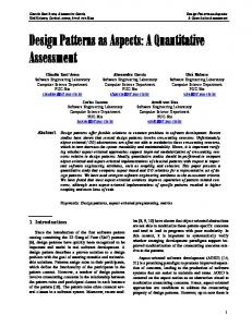
Fig. 1. (a) A 12.5 ms speech waveform of male voice, phoneme /a/, (b) laryngograph waveform, (c) estimated glottal volume velocity, and (d) autocorrelation LPC residual from preemphasised speech.
The accurate identification of GCIs has been an aim of speech researchers for many years and numerous techniques have been proposed. The most widely used approach is to look for discontinuities in a linear model of speech production [11]–[14]. An alternative is to search for energy peaks in waveforms derived from the speech signal [8], [15], [16] or for features in its time-frequency representation [17], [18]. To obtain good results in closed-phase speech processing, it is essential to identify the time of glottal excitation at closure to within a fraction of 1 ms whereas locating the precise glottal opening instant is normally much less critical [3], [10], [19]. In Fig. 1, waveform (a) shows a 12.5 ms segment of male speech from the vowel /a/. Waveform (b) shows a simultaneous Laryngograph recording (also called Electroglottograph or EGG) which measures the electrical conductance of the larynx at 2 MHz and provides a direct indication of glottal activity [5], [20]. The positions of the glottal closure and opening instants are indicated on this waveform as P and Q, respectively, and the interval PQ is the closed phase of the larynx cycle. Acoustic theory shows that, for vowel sounds, the vocal tract acts as an all-pole filter whose input is the volume velocity (also called volume flow rate) of air through the glottis [21]. The estimate of this volume velocity shown as waveform (c) was obtained by applying covariance LPC to the closed-phase speech segment PQ, filtering the speech by the resultant all-zero inverse filter and then applying a leaky integrator to the result to compensate for lip radiation [13], [21]. By restricting the analysis to the closed-phase in this way, we obtain an estimate of the vocal tract filter that is unperturbed by the glottal excitation. The low frequency fidelity of the volume velocity waveform estimate can be improved by correcting for phase distortion in the recording process [22] but the important features can be seen in the uncorrected waveform, namely a rapid decrease at glottal closure (P) and a less abrupt increase at opening (Q). Waveform (d) is the LPC residual obtained by applying the LPC inverse filter to a preemphasised speech waveform. The use of preemphasis and the omission of any compensation for
1558-7916/$20.00 © 2006 IEEE
Authorized licensed use limited to: Imperial College London. Downloaded on January 4, 2010 at 08:12 from IEEE Xplore. Restrictions apply.
BROOKES et al.: GROUP DELAY METHODS FOR IDENTIFYING GLOTTAL CLOSURES IN VOICED SPEECH
lip radiation mean that the waveform is approximately equal to the second derivative of the volume velocity. It can be seen that this waveform includes an impulsive feature at closure (P) and a similar but smaller impulse at opening (Q). The use of this LPC residual waveform for detecting glottal closure instants using methods such as those proposed in [12]–[14], [23]–[25] requires the following assumptions: (i) the vocal tract acts as an all-pole filter, (ii) the filter can be estimated adequately from the speech waveform alone and (iii) the LPC residual will contain an identifiable impulse at closure for voiced speech sounds. Assumptions (i) and (ii) are discussed later in this Section. The main contributions of this paper are (a) to demonstrate that assumption (iii) is correct for a large proportion of larynx cycles, (b) to introduce a new energy-weighted group-delay measure as a means of locating the impulse, (c) to give a quantitative assessment of the new measure’s performance and a comparative evaluation of three other measures based on group-delay, and (d) to provide efficient recursive algorithms for the computation of all four measures. The all-pole filter model of the vocal tract is less good for voiced consonants than for vowel sounds for two reasons. Firstly, the closed oral cavity in nasal consonants introduces zeros into the vocal tract filter response. For these phonemes therefore, the the vocal tract is poorly modeled and in some speakers closure impulses are not apparent in the residual. A method is proposed in [26] for improving the robustness of the LPC analysis in these cases by averaging the inverse filters obtained for different orders but this has not been evaluated in this study. Secondly, in voiced consonants there are often additional excitations arising from turbulence at points of vocal tract constriction. The effect of these on the speech signal is equivalent to the addition of colored noise onto the glottal volume velocity waveform. This noise will partially mask the closure impulses and may also have an adverse effect on the filter obtained from the LPC analysis. It is our experience however, that these phonemes nevertheless generate detectable energy peaks in the LPC residual at closure; this is confirmed by the results reported in Section IV. Although covariance LPC is preferred for estimating inverse filtered waveforms such as Fig. 1(c) [13], we have used autocorrelation LPC to derive the residual signal that is used for GCI detection because it offers increased robustness and has less sensitivity to the alignment between analysis frames and larynx cycles [27]. The use of a group delay measure to determine the acoustic excitation instants was first proposed in [23] and later refined in [24] and [25]. The method calculates the frequency-averaged group delay over a sliding window applied to the LPC residual. It has been found to be an effective way of locating the GCIs and the authors have demonstrated its robustness to additive noise. The technique was extended in [28], [29] in order to capture GCIs that were missed by the original algorithms and, through the use of dynamic programming, to eliminate spurious detections so as to identify more reliably those that correspond to true glottal closures rather than to glottal openings or other events. In [2], two alternative methods of identifying excitation instants were proposed, both related to the group delay. These were applied to the problem of inter-segment coherence in concatenative speech synthesis.
457
In Section II we define the four group delay measures to be evaluated in this paper. Three of these have been described elsewhere [2], [25] and the fourth is a new energy-weighted measure which we introduce here. In Section III we examine the theoretical properties of the measures and illustrate aspects of their behavior using synthetic signals. In Section IV we provide a quantitative evaluation of their performance in identifying GCIs in real speech. Included in our database recordings is a Laryngograph signal which provides a direct measurement of glottal activity and allows an objective assessment of accuracy. We examine in detail the effects of analysis window length on performance and we identify the tradeoffs that exist between detection rate and timing accuracy. We also evaluate the use of input signals other than the LPC residual. In Section V we examine the computational cost of evaluating the measures and we propose new efficient recursive procedures that significantly reduce this cost. II. GROUP DELAY , we consider an Given an input signal dowed segment beginning at sample
-sample win(1)
The Fourier transform of
at a frequency
is (2)
where can vary continuously. The group delay of given by [24]
is
(3) where is the Fourier transform of . The motivation for using the group delay is that it is able to identify the position of an impulse within the analysis window. , where is the unit impulse function, If . In the then it follows directly from (3) that will no longer be constant and presence of noise, however, we need to form some sort of average over . In Section II-A, we sample the spectrum by restricting to integer values and we , , and that perform describe four measures, this averaging in different ways to generate alternative estimates of the delay from the start of the window to the impulse. A. Average Group Delay The frequency-averaged group delay is given by
Authorized licensed use limited to: Imperial College London. Downloaded on January 4, 2010 at 08:12 from IEEE Xplore. Restrictions apply.
(4)
458
IEEE TRANSACTIONS ON AUDIO, SPEECH, AND LANGUAGE PROCESSING, VOL. 14, NO. 2, MARCH 2006
where the conjugate symmetry of and ensures that the was proposed in [23] as latter summation is real. The use of a way of estimating the GCIs and was later refined in [24] and [25]. Direct evaluation of (4) requires two Fourier transforms per output sample but the computation may be reduced by the recursive formulae given in Section V. A disadvantage of this approaches zero for some , then the measure is that if resultant quotient will dominate the summation in (4) and may result in a very large value for . To avoid such extreme values we have found it essential to follow the recommendation in [25] that a 3-term median filter be applied to along the axis before performing the summation in (4). B. Zero-Frequency Group Delay was proposed in [2] as a way of The group delay at estimating the instant of excitation and is given by
. The which may be viewed as the “center of energy” of , thus has an efficient time-domain fornew measure, mulation. Unlike the previous measures it is bounded and lies provided that is not identically in the range 0 to zero. D. Energy-Weighted Phase Equation (8) may be viewed as a weighted average of using as the weighting factors. An alternative way of averaging is to associate the sample positions within the window with complex numbers of the form , evenly spaced around the unit circle on the complex plane. To form the energy-weighted phase, we take a weighted average of these as the weighting factors and then complex numbers using to convert back to a delay. This multiply its argument by gives (9)
(5)
This measure may be interpreted as the “center of gravity” of . Although easy to calculate, it is, as we shall see, sensitive to noise and its value is unbounded if the mean value of approaches zero. Because of this, we have found it necessary to after evaluating (5). apply a median filter to C. Energy-Weighted Group Delay The problem of unbounded terms in the summation of (4) , the may be circumvented by weighting each term by energy at frequency index . This leads us to propose a new measure, the energy-weighted group delay, defined by
(6)
. The discontinuity in has been where chosen to lie midway between the complex numbers associated and . It is clear from (9) that with always lies in the range to . A measure similar to was used in [2] for aligning waveform segments in a speech synthesis system. The relationship to the energy-weighted group delay as described above and the noise immunity described in Section III-B provide useful new insights into the properties of this measure. III. PROPERTIES OF GROUP DELAY MEASURES In Section IV we will use the delay measures defined above to identify the excitation instants in the LPC residual from real speech. In this Section however, we gain insight into their properties by examining their behavior with synthetic signals that consist of impulses with additive white Gaussian noise. The properties that we observe are consistent with those reported in [23], [25] but we extend the study here to include an analysis of multiple impulses and a quantitative comparison between the different measures. A. Effect of Window Length An idealized version of the LPC residual waveform is shown as in Fig. 2(a) and consists of an impulse train with additive white Gaussian noise at 10 dB SNR. The dominant pulse period is 100 samples with an additional pulse in the fourth period and with the amplitude of the third pulse half that of the others. It is convenient to shift the time-origin of the sliding window, in (1), to its central point by defining
This expression may be simplified by noting that
(7)
(10) where
Substituting this into (6) gives
(8)
is one of . Note that if is even, is defined for values of midway between the integers must always be an integer. since the argument of for four difFig. 2(b)–(e) shows the waveform of is chosen to ferent values of window length, , where be a symmetric Hamming window of period . The effect of
Authorized licensed use limited to: Imperial College London. Downloaded on January 4, 2010 at 08:12 from IEEE Xplore. Restrictions apply.
BROOKES et al.: GROUP DELAY METHODS FOR IDENTIFYING GLOTTAL CLOSURES IN VOICED SPEECH
459
Fig. 2. (a) Impulse train with a dominant period of 100 samples and an SNR of 10 dB. (b)–(e) the waveform of for different window lengths, . The circles mark the negative-going zero crossings (NZCs).
varying the window length is broadly similar for all measures, . so we will discuss it in detail only for All four measures from Section II give the correct result for a then . noise-free impulse; i.e., if All the measures also possess a form of shift invariance so that and then if (11) and so the graph of has a gradient of under these circumstances. Although these conditions do not quite hold in this example because of the added noise, they are almost true when does not an impulse is near the center of the window and exceed the impulse period. For these cases therefore, we see in has a negative-going zero crossing Fig. 2(b) and (c) that whenever an im(NZC) with a gradient of approximately . Each NZC is marked with a circle. pulse is present at In Fig. 2(c), the window size equals the period resulting in a clearly defined NZC for each impulse without the introduction of any spurious NZCs. However when the window size is much less than the period as in Fig. 2(b), there are intervals between each impulse where the window contains only is almost flat and numerous spunoise. In these intervals rious NZCs are introduced. The local gradient at these spurious and this provides a possible NZCs is close to 0 rather than way of identifying them. As the window size is increased, it becomes common for two or more impulses to lie within the window and individual impulses may no longer be resolved. Thus in Fig. 2(d) where , we see that the two impulses that are closest together (40 samples separation) have resulted in a single NZC approximately midway between them. As the window length is increased further in Fig. 2(e), each impulse now contains only a small fraction of the energy in the window. This means that the waveform is low and the timing accuamplitude of the racy with which impulse locations can be identified degrades. In this example, the low amplitude third impulse contains so little energy compared to other nearby pulses that it fails to generate an NZC at all. The example of Fig. 2 therefore illustrates the way in which to detect impulses depends on the ratio of the ability of the window length to the input signal period. As we shall see in Section IV the choice of window length is a compromise: a window that is too short will introduce many spurious NZCs while a window that is too long may result in failure to detect some of the true GCIs.
Fig. 3. Variation of , , and as the signal-to-noise ratio to for an input consisting of a single impulse (SNR) varies from with additive white Gaussian noise in a window length of . at For each measure, the graph shows the median value of and the upper and lower quartiles.
B. Robustness to Noise To assess the effect of noise on the delay measures, we have applied them to a signal consisting of a single impulse with additive white Gaussian noise. Fig. 3 shows the behavior of each to for an immeasure as the SNR is varied from within a rectangular window of length pulse at sample . For each measure, the corresponding graph shows and the upper and lower quartiles. We the median value of use the median rather than the mean because of the unbounded and . At an SNR of values sometimes generated by all measures correctly give with a very small inter-quartile range. As the SNR is reduced all measures show an increasing spread and a progressive bias with the median values tending to 50, the center of the window. The most robust whose median value is barely affected by noise measure is . For this measure, the effect of until the SNR falls below the noise is to add onto the summation in (9) a random complex number of arbitrary phase. It follows that the noise will not afunless the noise amplitude is large fect the median value of enough to cause the value of the summation to cross the positive function. real axis where there is a discontinuity in the For impulses near the centre of the window, the summation in (9) lies on or near the negative real axis and so for positive SNR . values, the noise has little effect on the median of The measure whose median is most sensitive to noise is for which the effects are noticeable in Fig. 3 for SNRs as high as 14 dB. Since this measure calculates the center of energy of the windowed signal, the bias introduced depends directly on the will be halfway SNR and at an SNR of 0 dB, for example, between and the window center. The median curves for and are almost identical to each other and lie between those of the other two measures with significant bias only for SNRs worse than 5 dB. Although low levels of noise have little effect , they have a substantial effect on on the median value of its inter-quartile range which is considerably larger than that of the other measures. When noise is added to an impulse train like that in Fig. 2(a) the NZCs are affected in two ways. Firstly, the bias toward the is pulled toward zero either side window center means that of the NZC and so its gradient will be less steep. It is possible,
Authorized licensed use limited to: Imperial College London. Downloaded on January 4, 2010 at 08:12 from IEEE Xplore. Restrictions apply.
460
IEEE TRANSACTIONS ON AUDIO, SPEECH, AND LANGUAGE PROCESSING, VOL. 14, NO. 2, MARCH 2006
Fig. 4. Graph shows, as a function of SNR, how far an impulse must be from , , and the center of a 101 sample window to ensure that have the correct sign with a probability of 75%.
therefore, to use the gradient of at an NZC to estimate the SNR of the signal. The second effect is that the combination of the bias and the increased variance will add uncertainty to the position of the NZC. Fig. 4 shows, as a function of SNR, how far an impulse must be from the center of a 101 sample window for the upper or lower quartile to lie exactly at the center of the window, i.e., how far the impulse must be from the center for to have a probability of 0.75 of having the correct sign. We can view this as a measure of how accurately the position of the impulse will be located and of how this accuracy degrades with noise. The algorithms attain a precision of 5 samples (5% of the window length) with 75% probability at SNR levels of , and for the , , and 11.9, measures, respectively. This indicates that the timing of and is most the NZCs is least affected by noise when using affected when using . C. Response to Multiple Impulses It is possible for the analysis window to contain multiple impulses either because the window is longer than the pulse period or because, as is often the case with the LPC residual, the signal includes additional pulses or other impulsive features. We consider here the behavior of the measures when the window contains two impulses. From the shift invariance property, (11), we may, without loss of generality take the impulses to be at posigiving tions (12) where the factor lies in the range 0 to 1 and determines the relative amplitude of the two impulses. We can evaluate the four measures analytically (see Appendix) to obtain the following exact results. It is convenient to express them in terms of which ranges from 0 to and is the negative of the ratio of the impulse magnitudes
(13)
Fig. 5. Values of , , and for a signal containing impulses and , respectively. The window length at samples 0 and 40 of amplitudes is 101 and varies between 0 and 1.
where denotes the greatest common divisor and the equation for should be regarded as modulo with . Fig. 5 plots the expressions from and . (13) versus for the particular case of to As varies from 0 to 1 all the measures change from . Measure equals the center of gravity of the pair of impulses and it therefore changes linearly with . Meaon the other hand, which equals the center of gravity sure of the squared input signal, is biassed toward the position of the larger impulse giving rise to the S-shaped curve shown. In the , the exponent of depends on expression for and is, for this case, equal to 101. Because this is so high, makes an extremely abrupt transition at and this measure essentially locates the position of the highest peak in the window. It is possible to obtain a similar behavior for or by increasing the exponent of in (8) or (9) but we have found that this does not improve their performance with real speech and so we do not discuss the resultant measures in varies according to the separation detail. The behavior of of the two impulses. When they are close to each other it is but as their separation increases to almost the same as half the window length its graph approaches that of . For the graph changes completely and separations greater than decreases toward , wrapping as increases from 0, then continuing down to . around abruptly to IV. EVALUATION WITH SPEECH SIGNALS The four measures defined in Section II have been evaluated using the sentence subset of the APLAWD database [30] recorded anechoically at a sample rate of 20 kHz with a lip-tomicrophone distance of 15 cm. The database includes a Laryngograph channel which provides a direct measurement of glottal activity [5], [20] and allows the instants of glottal closure to be determined using the HQTx program from the Speech Filing System software suite [31], [32]. The database includes ten repetitions from each of ten British English speakers (five male, five female) of the following sentences: S1: “George made the girl measure a good blue vase;” S2: “Why are you early you owl?” S3: “Cathy hears a voice amongst SPAR’s data;” S4: “Be sure to fetch a file and send their’s off to Hove;” S5: “Six plus three equals nine;”
Authorized licensed use limited to: Imperial College London. Downloaded on January 4, 2010 at 08:12 from IEEE Xplore. Restrictions apply.
BROOKES et al.: GROUP DELAY METHODS FOR IDENTIFYING GLOTTAL CLOSURES IN VOICED SPEECH
461
Fig. 6. Histogram of larynx cycle periods for male and female speakers.
for a total of 500 utterances. Ten of the utterances contained recording errors and, after excluding voiced segments with fewer than five cycles, the remaining 490 utterances contained 129 537 glottal closures whose times were delayed by 1 ms to provide a first order correction for the larynx-to-microphone delay. Fig. 6 shows the histograms of larynx period for the male and the female speakers obtained from HQTx. A. Waveform Processing Fig. 7 shows (a) a segment of speech with (b) the Laryngograph waveform, (c) the LPC residual, , and (d) the waveform with its zero-crossings (NZCs) marked by circles. The of Laryngograph waveform measures the electrical conductance of the larynx and shows an abrupt increase at glottal closure. The boundaries of the larynx cycles are placed midway between adjacent closures and are shown as vertical dashed lines. The speech is first passed through a 1st order preemphasis filter with a 50 Hz corner frequency and then processed using autocorrelation LPC of order 22 with 20 ms Hamming windows overlapped by 50%. We use autocorrelation rather than covariance LPC to reduce sensitivity to the position of larynx cycles within the window. The preemphasised speech is inverse filtered with linear interpolation of the LPC coefficients for 2.5 ms either side of the frame boundary. Finally, in order to remove high frequency noise, the residual is lowpass filtered at 4 kHz using .A a second-order Butterworth filter to obtain the signal sliding Hamming window is applied to and the delay measures from Section II are calculated. The energy weighting, median filter and 1.5 kHz low pass filter recommended in [25] measure and a 3-point median filter are applied to the is also applied to in order to remove the extreme values that are sometimes generated. The speech segment of Fig. 7 has been chosen to illustrate some of the difficulties that arise in detecting the GCIs. Identifying the GCIs has proved more difficult for this particular male speaker than for any of the other speakers in our database. His speech sometimes contains an unusually strong excitation at glottal opening which, as can be seen from the LPC residual waveform in Fig. 7(c), may be comparable in strength to the excitation at glottal closure. In each of the first four larynx cycles a strong excitation is visible in the LPC residual at glottal cloat or near the sure and this results in a well-defined NZC in center of the cycle. In the second four larynx cycles, the poor signal-to-noise ratio of the LPC residual results in a low amplitude waveform. In these cycles, the secondary excitation at
Fig. 7. (a) Segment of male speech from diphthong/aI/with (b) the Laryngograph waveform, (c) the LPC residual, and (d) the waveform of with NZCs identified by circles. The vertical dashed lines indicate the larynx cycle boundaries.
glottal opening gives rise to an additional NZC and in the penultimate cycle, the excitation at glottal closure is so weak that no is visible. It is possible NZC results although a ripple in to use the projection technique described in [28], [29] to determine NZC-equivalent time instants from the turning points of such ripples but this is outside the scope of this study. The waveforms of Fig. 7, appear to indicate the possibility of using to detect the glottal opening instants (GOIs) in addition to the GCIs. However, in many other speakers, the GOI excitations are very small and so the reliable identification of GOIs remains a very challenging task with, as yet, little reported work in the literature. The present study is aimed specifically at distinguishing the GCI excitations and for this reason we regard any NZCs arising from the GOIs as unwanted errors. B. Timing Error Histograms In most larynx cycles, the measures will generate a single NZC at or near the instant of glottal closure. If, for example a window length of 8 ms is used, then about 88% of larynx cycles give exactly one NZC in . Fig. 8(a) shows a histogram of the deviation of the NZC from the true larynx closure as determined using HQTx applied to the Laryngograph signal. The mean value is close to zero which confirms the value of 1 ms used for the larynx-to-microphone delay compensation. The standard deviation is 0.55 ms, but the underlying accuracy of the GCI estimation is somewhat better than this because variations in the larynx-to-microphone acoustic delay due to head movement can add as much as 0.1 ms onto this figure. Of the remaining 12% of larynx cycles, over three quarters contain exactly two NZCs; in most cases these occur at glottal opening and closure, respectively, giving rise to the histogram shown in Fig. 8(b). The standard deviation of this tri-modal distribution is not a useful measure. Instead, we consider in our statistics only the NZC in each larynx cycle that is closest to the GCI and make the assumption that the other NZC can be rejected using techniques such as those described in [28], [29]. For this example, the standard deviation of these “closest” NZCs is 0.97 ms and if we combine these with the single-NZC cycles, we can detect the GCI in over 97% of larynx cycles with a standard deviation of 0.6 ms. The remaining 3% of cycles either contain more than
Authorized licensed use limited to: Imperial College London. Downloaded on January 4, 2010 at 08:12 from IEEE Xplore. Restrictions apply.
462
IEEE TRANSACTIONS ON AUDIO, SPEECH, AND LANGUAGE PROCESSING, VOL. 14, NO. 2, MARCH 2006
Fig. 8. Histograms of the deviation between the instant of glottal closure and the zero crossings (NZCs) of . Histograms (a) and (b) are for larynx cycles containing exactly one and exactly two NZCs, respectively. Fig. 10. Detection rate and detection accuracy for cycles containing either one or two NZCs. For each algorithm the window length varies from 4 ms (leftmost point) to 13 ms in steps of 1 ms.
Fig. 9. Identification rate and identification accuracy for cycles containing exactly one NZC. For each measure the window length varies from 4 ms (leftmost point) to 13 ms in steps of 1 ms.
two NZCs or else contain none at all and we assume, pessimistically, that the glottal closure instant cannot be identified for any of these cycles. C. Accuracy and Detection Rate We define the identification rate of a measure to be the fraction of larynx cycles that contain exactly one NZC and the detection rate to be the fraction that contain either one or two NZCs. Thus in Fig. 7, for example, the identification rate is 50% and the detection rate is 100%. We consider that the detection rate gives a good assessment of the potential of the measure to locate the GCIs provided that techniques such as those from [28], [29] are used to reject the NZCs associated with glottal opening. The identification accuracy is the standard deviation of the timing error between the GCI and the NZC for cycles containing exactly one NZC. The detection accuracy is the standard deviation of the timing error between the GCI and the closest NZC for cycles containing either one or two NZCs. In Fig. 9 we plot the identification rate against the identification accuracy for each of the four algorithms for window lengths varying between 4 ms and 13 ms in steps of 1 ms. Each curve is labeled with its algorithm abbreviation and in all cases the leftmost point corresponds to the shortest window (4 ms). The curves labeled “EPF” and “EPS” use alternative input signals and are discussed in Section IV-E. To take a specific example, measure is identified by circles and we see from the first the point on the graph that for a 4 ms window, its identification accuracy is 0.34 ms but its identification rate is only 36%. This low rate arises because with a window as short as this, most larynx
cycles will contain more than one NZC. As the window length in increased the accuracy steadily worsens but the identification rate improves and reaches a peak of over 90% at a window length of 10 ms. Beyond this point, the identification rate falls again as an increasing number of cycles contain no NZC at all. measure is almost identical to that The performance of the of the measure but reaches its peak at the shorter window measure has a somewhat worse perforlength of 8 ms. The meamance and only achieves a peak of 83.2% while the sure is by far the worst with a peak identification rate of only 55% and a substantially worse accuracy. In Fig. 10, we show the same curves but this time for the detection rate and detection accuracy that are based on the larynx and cycles that contain either one or two NZCs. The measures again show the best performance and reach a detection rate of 97.1% for window lengths of 8 ms and 7 ms, respectively. measure is slightly worse with a peak detection rate of The measure reaches a peak of 90%, 94.6% and although the its detection accuracy is off the graph at 1.4 ms. In general, as the window length is decreased, the number of NZCs rises and accuracies improve. It is not surprising, therefore, that for all measures the peak detection rate has a better accuracy than the peak identification rate and occurs with a window length that is between 1 ms and 2 ms shorter. D. Gender and Linguistic Content Differences In Fig. 11, the detection rate is shown for each of the ten speakers as a function of the window length using the measure. It can be seen that the female speakers (marked with circles) are closely bunched and the peak detection rate is achieved with a window length of between 6 and 7 ms. The male speakers are less tightly bunched and have slightly worse detection rates than the female speakers with peak performance occurring at window lengths between 7 and 10 ms. The male speaker used in the example of Fig. 7 shows the poorest detection rate. His speech is notable for the high proportion of cycles that include a strong excitation at glottal opening and in consequence his speech also shows the worst identification rate. If a single window is used for all speakers, then the optimum compromise is a window length of 8 ms. If the best window length is used for each speaker the detection rate for the measure rises from 97.1% to 97.8% with the identification rate
Authorized licensed use limited to: Imperial College London. Downloaded on January 4, 2010 at 08:12 from IEEE Xplore. Restrictions apply.
BROOKES et al.: GROUP DELAY METHODS FOR IDENTIFYING GLOTTAL CLOSURES IN VOICED SPEECH
463
can be to those reviewed in [33]. Many popular windows, expressed as the sum of a small number of exponentials (14)
Fig. 11. Detection rate for as a function of window length. A separate curve is shown for each female (circles) and male (crosses) speaker.
remaining at 87.4%. It is therefore likely that the use of an auxiliary pitch estimator and an adaptive window length would give a modest improvement in performance. measure on indiEvaluating the performance of the vidual sentences revealed only one significant difference. The fully voiced sentence, S2, gave a slightly higher detection rate (97.8%) with much better accuracy (0.45 ms) than the other sentences which all gave similar results of 97% and 0.62 ms. We have not analyzed the reasons for this in detail but we suggest that the lack of frication in sentence S2 may be a contributory factor. E. Alternative Input Signals The group delay measures may be applied to any signal containing an energy peak at the time of glottal closure. We include in Figs. 9 and 10 the results of applying the measure to the preemphasized speech (EPS) and to the estimated glottal energy flow (EPF). The use of the preemphasized speech energy to detect glottal closures was proposed in [15] and the estimation of the glottal energy flow is described in [8]. We see that applying measure to these signals gives good results and that the the peak identification and detection rates were, respectively, 92.6% and 97.7% for EPS and 87.2% and 97.4% for EPF. The identification rate for EPS and the detection rates for both EPF and measure is EPS are higher than those obtained when the applied to the LPC residual but this improvement comes at the cost of poorer accuracy. It can also be seen that as the window length is decreased below 8 ms, the EPF identification rate decreases very rapidly while its detection rate remains well above 90% even for windows as short as 4 ms. This behavior means that the EPF measure is detecting exactly two acoustic excitations in a large fraction of cycles and indicates that it could potentially be effective in identifying the closed phase intervals. measure on unpreemphasized We have also evaluated the speech but, with peak identification and detection rates of 85% and 96%, respectively, this did not perform as well as EPS.
V. EFFICIENT COMPUTATION In this section, we present efficient recursive algorithms for calculating the group delay measures using techniques similar
For example, a centered Hamming window with period (rather than the commonly used period of ) has and . The are the inverse and in a similar discrete Fourier transform coefficients of to be the IDFT coefficients of . For way we define such windows, we will derive efficient recursive formulae for . the quantities If we define (15) we can derive the relationships
We can use these to calculate the and recursively although in practice, the recursions must be reinitialized periodically using (15) to avoid cumulative errors. Having calculated the and , we can use the following relationships to evaluate the measures:
(16) with similar expressions for and the Fourier transform of involving . Additional savings can be made by using the conjugate symmetry of the , , and . Table I shows the number of flops per sample reported by MATLAB when evaluating the four measures using both direct and recursive forms of evaluation for a window length of 101. The figures include the median filtering that is essential for and . The figures for are somewhat lower than they should be since MATLAB budgets only one flop for the function in (9). For the recursive forms, the computational costs , and are independent of whereas those of are proportional to . The savings from the recursive for but even so this measure is by formulation is greatest for far the most costly to compute. VI. CONCLUSION In this paper, we have investigated four measures of group delay and their use for GCI estimation. Three of these measures have been described in earlier publications and one is newly
Authorized licensed use limited to: Imperial College London. Downloaded on January 4, 2010 at 08:12 from IEEE Xplore. Restrictions apply.
464
IEEE TRANSACTIONS ON AUDIO, SPEECH, AND LANGUAGE PROCESSING, VOL. 14, NO. 2, MARCH 2006
TABLE I COMPUTATIONAL COST IN FLOPS PER SAMPLE FOR DIRECT AND RECURSIVE , , AND FOR A IMPLEMENTATIONS OF MEASURES WINDOW LENGTH
proposed here. We have evaluated their behavior with synthetic data and their ability to detect GCIs in real speech. From the experiments with synthetic data, we found that additive noise increases the variability of all the measures and biases measure is their value toward the center of the window. The is by far the most the least sensitive to additive noise while sensitive. To detect GCIs in real speech, we applied the measures to the LPC residual using a sliding window and identified the negative-going zero-crossings (NZCs) of the time-aligned . The and measures performed exmeasures ceptionally well and, using the optimum fixed window length, generated either one or two NZCs in over 97% of larynx cycles. About 9% of these cycles contained two NZCs and in most cases these corresponded to excitations at glottal closure and opening, respectively. The standard deviation of the timing error between the true GCI and the closest NZC was about 0.6 ms; this figure overestimates the true timing inaccuracy since it includes variations in the larynx-to-microphone acoustic delay arising from head movement. If the optimum window length is used for each speaker, the detection rate rises to 97.8% and it is expected that this would rise further if the window length were adapted to the pitch. The detection rate shows little dependence on linguistic content but the detection accuracy was much better for a sentence that was fully voiced sentence without frication. measure to the We have evaluated the application of the raw speech, the preemphasized speech and the glottal energy flow waveforms in addition to the LPC residual. We found that the highest accuracies were obtained with the LPC residual but that the highest identification rate (92.6%) and detection rate (97.7%) were obtained from the preemphasized speech. The glottal energy flow waveform showed the greatest robustness to window length variation and, for short windows, had the highest proportion of cycles with two NZCs indicating potential advantages in identifying glottal opening instants and closed phase intervals. We have shown how the computational cost of all the measures can be reduced greatly by calculating them recursively provided that a suitable window function is used. Even so, the measure is around 100 times greater than that cost of the of the others. and which Overall, our preferred measures are have virtually identical performance on real speech. The measure has better theoretical noise immunity but is somewhat more costly to evaluate and was slightly less robust to short window lengths. Despite the good performance obtained from the measures studied in this paper, they do not provide a complete solution to the problem of detecting GCIs. To eliminate the NZCs corresponding to glottal opening and those generated during unvoiced speech segments, it is necessary to combine them with a selection procedure such as that described in [28], [29].
APPENDIX RESPONSE TO A NOISEFREE DUAL IMPULSE In this appendix we prove the expressions given in (13) for the response of the group delay measures to a dual impulse. We assume that the input signal is given by
and we define We may write
For convenience we now define
.
giving
from which we obtain the following equation modulo
where must lie in the range Finally we observe that iff This in turn is true iff is a multiple of follows that for
Authorized licensed use limited to: Imperial College London. Downloaded on January 4, 2010 at 08:12 from IEEE Xplore. Restrictions apply.
is a multiple of
. . . It
BROOKES et al.: GROUP DELAY METHODS FOR IDENTIFYING GLOTTAL CLOSURES IN VOICED SPEECH
We may now write
ACKNOWLEDGMENT The authors would like to thank the anonymous referees for their useful comments. REFERENCES [1] C. Hamon, E. Moulines, and F. Charpentier, “A diphone synthesis system based on time-domain prosodic modifications of speech,” in Proc. ICASSP, Glasgow, U.K., May 1989, pp. 238–241. [2] Y. Stylianou, “Synchronization of speech frames based on phase data with application to concatenative speech synthesis,” in Proc. 6th Eur. Conf. Speech Communication and Technology, vol. 5, Budapest, Hungary, Sep. 1999, pp. 2343–2346. [3] K. Steiglitz and B. Dickinson, “The use of time-domain selection for improved linear prediction,” IEEE Trans. Acoust., Speech, Signal Process., vol. ASSP-25, no. 1, pp. 34–39, Feb. 1977. [4] T. V. Ananthapadmanabha and B. Yegnanarayana, “Epoch extraction from linear prediction residual for identification of closed glottis interval,” IEEE Trans. Acoust., Speech, Signal Process., vol. ASSP-27, no. 4, pp. 309–319, Aug. 1979. [5] A. K. Krishnamurthy and D. G. Childers, “Two-channel speech analysis,” IEEE Trans. Acoust., Speech, Signal Processing, vol. ASSP-34, pp. 730–743, Aug. 1986. [6] B. Yegnanarayana and R. Veldhuis, “Extraction of vocal-tract system characteristics from speech signals,” IEEE Trans. Speech Audio Process., vol. 6, no. 4, pp. 313–327, Jul. 1998. [7] J. McKenna and S. Isard, “Tailoring Kalman filtering toward speaker characterization,” in Proc. Eurospeech, 1999, pp. 2793–2796. [8] D. M. Brookes and H. P. Loke, “Modeling energy flow in the vocal tract with applications to glottal closure and opening detection,” in Proc. ICASSP, Mar. 1999, pp. 213–216. [9] T. F. Quatieri, C. R. Jankowski, Jr, and D. A. Reynolds, “Energy onset times for speaker identification,” IEEE Signal Process. Lett., vol. 1, no. 11, pp. 160–162, Nov. 1994. [10] A. Neocleous and P. A. Naylor, “Voice source parameters for speaker verification,” in Proc. Eur. Signal Processing Conf., Rhodes, Greece, Sep. 1998. [11] M. D. Plumpe, T. F. Quatieri, and D. A. Reynolds, “Modeling of the glottal flow derivative waveform with application to speaker identification,” IEEE Trans. Speech Audio Process., vol. 7, no. 5, pp. 569–586, Sep. 1999. [12] H. Strube, “Determination of the instant of glottal closure from the speech wave,” J. Acoust Soc. Amer., vol. 56, no. 5, pp. 1625–1629, 1974. [13] D. Y. Wong, J. D. Markel, and A. H. Gray, Jr, “Least squares glottal inverse filtering from the acoustic speech waveform,” IEEE Trans. Acoust., Speech, Signal Process., vol. ASSP-27, no. 4, pp. 350–355, Aug. 1979.
465
[14] J. G. McKenna, “Automatic glottal closed-phase location and analysis by Kalman filtering,” in Proc. 4th ISCA Tutorial and Research Workshop on Speech Synthesis, Aug. 2001. [15] C. Ma, Y. Kamp, and L. F. Willems, “A Frobenius norm approach to glottal closure detection from the speech signal,” IEEE Trans. Speech Audio Process., vol. 2, no. 2, pp. 258–265, Apr. 1994. [16] C. R. Jankowski Jr, T. F. Quatieri, and D. A. Reynolds, “Measuring fine structure in speech: Application to speaker identification,” in Proc. ICASSP, May 1995, pp. 325–328. [17] V. N. Tuan and C. d’Alessandro, “Robust glottal closure detection using the wavelet transform,” in Proc. Eur. Conf. Speech Technology, Budapest, Hungary, Sep. 1999, pp. 2805–2808. [18] J. L. Navarro-Mesa, E. Lleida-Solano, and A. Moreno-Bilbao, “A new method for epoch detection based on the Cohen’s class of time frequency representations,” IEEE Signal Process. Lett., vol. 8, no. 8, pp. 225–227, Aug. 2001. [19] J. N. Larar, Y. A. Alsaka, and D. G. Childers, “Variability in closed phase analysis of speech,” in Proc. ICASSP, Mar. 1985, pp. 1089–1092. [20] E. R. M. Abberton, D. M. Howard, and A. J. Fourcin, “Laryngographic assessment of normal voice: A tutorial,” Clin. Linguist. Phon., vol. 3, pp. 281–296, 1989. [21] L. R. Rabiner and R. W. Schafer, Digital Processing of Speech Signals. Englewood Cliffs, NJ: Prentice-Hall, 1978. [22] M. J. Hunt, “Automatic correction of low-frequency phase distortion in analogue magnetic recordings,” Acoust. Lett., vol. 2, pp. 6–10, 1978. [23] R. Smits and B. Yegnanarayana, “Determination of instants of significant excitation in speech using group delay function,” IEEE Trans. Speech Audio Process., vol. 3, no. 5, pp. 325–333, Sep. 1995. [24] B. Yegnanarayana and R. Smits, “A robust method for determining instants of major excitations in voiced speech,” in Proc. ICASSP, Detroit, MI, 1995, pp. 776–779. [25] P. S. Murthy and B. Yegnanarayana, “Robustness of group-delay-based method for extraction of significant instants of excitation from speech signals,” IEEE Trans. Speech Audio Process., vol. 7, pp. 609–619, Nov. 1999. [26] M. R. Zad-Issa and P. Kabal, “A new LPC error criterion for improved pitch tracking,” in Proc. IEEE Workshop Speech Coding, Pocono Manor, PA, Sep. 1997, pp. 1–2. [27] L. R. Rabiner, B. S. Atal, and M. R. Sambur, “LPC prediction error-analysis of its variation with the position of the analysis frame,” IEEE Trans. Acoust., Speech, Signal Process., vol. ASSP-25, no. 5, pp. 434–442, Oct. 1977. [28] A. Kounoudes, P. A. Naylor, and M. Brookes, “The DYPSA algorithm for estimation of glottal closure instants in voiced speech,” in Proc ICASSP, vol. 1, Orlando, FL, 2002, pp. 349–352. , “Automatic epoch extraction for closed-phase analysis of [29] speech,” in Proc 14th Int. Conf. Digital Signal Process., vol. 2, 2002, pp. 979–983. [30] G. Lindsey, A. Breen, and S. Nevard, “SPAR’s Archivable Actual-Word Databases,” Univ. College, London, U.K., 1987. [31] M. A. Huckvale, D. M. Brookes, L. Dworkin, M. E. Johnson, D. J. Pearce, and L. Whitaker, “The SPAR speech filing system,” in Proc. Eur. Conf. Speech Technology, vol. 1, Edinburgh, U.K., Sep. 1987, pp. 305–308. [32] M. Huckvale. (2000) Speech Filing System: Tools for Speech Research. Univ. College London, London, U.K.. [Online]. Available: http://www.phon.ucl.ac.uk/resource/sfs/ [33] E. Jacobsen and R. Lyons, “The sliding DFT,” IEEE Signal Processing Mag., vol. 20, no. 2, pp. 74–80, Mar. 2003.
Mike Brookes (M’88) received the B.A. degree in mathematics from Cambridge University, Cambridge, U.K., in 1972. Following this, he went to the U.S. where he spent four years at the Massachussets Institute of Technology, Cambridge, working on astronomical instrumentation and telescope control systems. Since 1979, he has worked in the Electrical and Electronic Engineering Department, Imperial College, London, U.K., where he is now a Deputy Head of Department and Head of the Communications and Signal Processing Research Group. His main areas of research is speech processing where he has worked on speech production modeling, speaker recognition algorithms and techniques for speech enhancement using both single microphones and microphone arrays. He is currently applying techniques from speech processing to RADAR target identification and is also actively involved in computer vision research.
Authorized licensed use limited to: Imperial College London. Downloaded on January 4, 2010 at 08:12 from IEEE Xplore. Restrictions apply.
466
IEEE TRANSACTIONS ON AUDIO, SPEECH, AND LANGUAGE PROCESSING, VOL. 14, NO. 2, MARCH 2006
Patrick A. Naylor (M’89) received the B.Eng. degree in electronics and electrical engineering from the University of Sheffield, Sheffield, U.K., in 1986 and the Ph.D. degree from Imperial College, London, U.K., in 1990. Since 1989, he has been a Member of Academic Staff in the Communications and Signal Processing Rsearch Group at Imperial College where he is also Director of Postgraduate Studies. His research interests are in the areas of speech and audio signal processing and he has worked in particular on adaptive signal processing for acoustic echo control, speaker identification, multi-channel speech enhancement and speech production modeling. In addition to his academic research, he enjoys several fruitful links with industry in the U.K., U.S., and mainland Europe. Dr. Naylor is an associate editor of the IEEE SIGNAL PROCESSING LETTERS and a member of the IEEE Signal Processing Society Technical Committee on Audio and Electroacoustics.
Jon Gudnason (M’04) received the B.Sc. and M.Sc. degrees in electrical engineering from the University of Iceland in 1999 and 2000, respectively. He is now pursuing the Ph.D. degree with the Communication and Signal Processing Group at Imperial College, London, U.K. From 1996 to 1998, he worked as intern with the Hydrology Service at the National Energy Authority in Iceland and in 1999 he worked as a Research Assistant for the Information and Signal Processing Laboratory at University of Iceland working on remote sensing applications. He is currently a Research Associate with the Communication and Signal Processing Group at Imperial College where his research has been on speaker recognition and automatic target recognition using radar. Mr. Gudnason is member of the IEEE Signal Processing Society. He was the president of the IEEE Iceland student branch in 1998.
Authorized licensed use limited to: Imperial College London. Downloaded on January 4, 2010 at 08:12 from IEEE Xplore. Restrictions apply.