A Quantitative Comparison between Traditional and Line ... - CiteSeerX

2538

MONTHLY WEATHER REVIEW

VOLUME 129

A Quantitative Comparison between Traditional and Line Integral Methods of Derivative Estimation PHILLIP L. SPENCER* Cooperative Institute for Mesoscale Meteorological Studies, University of Oklahoma, Norman, Oklahoma

CHARLES A. DOSWELL III1 NOAA/OAR National Severe Storms Laboratory, Norman, Oklahoma (Manuscript received 5 October 2000, in final form 18 April 2001) ABSTRACT For diagnostic purposes, the ‘‘traditional’’ approach to estimating derivatives employs objective analysis to provide a gridded field from the original observations, which are typically not uniformly distributed in space. However, there exist other methods involving derivative estimation via line integral (‘‘triangle’’) techniques that do not involve a prior mapping of the field onto a uniform grid. It has been suggested that these give improved results. Empirical testing of the differences between wind field derivative estimation using two different schemes is done with prototypical examples of the techniques. Test results verify that the triangle method indeed provides substantial improvements over the traditional scheme. The magnitude of the improvement is shown to depend on the degree of irregularity of the data distribution, as expected. Although the particular prototype methods chosen have the property that the triangle method truncates the amplitude of the input field slightly more than the traditional scheme, the pattern of the field is significantly better using the triangle technique than with the traditional method. An unexpected result is that the improvement by the triangle method over the traditional approach does not diminish as the wavelength of the input field increases. It is shown that this is a consequence of overfitting of the field to the station observations, causing local discontinuities in the field that produce errors in the gradient calculations, even in situations where the distribution of data is uniform. Overall, the test results make it abundantly clear that the traditional method is generally inferior to derivative estimates via the line integral methodology.

1. Introduction There are at least two reasons for performing what has been described as ‘‘objective analysis’’ on observations: 1) it is a part of the process used for initialization of numerical simulation models, and 2) it is perceived as the beginning of diagnostic analysis of the observations. In what follows, our primary emphasis is on the methods used for diagnosis of observed data when those observations are obtained from sites distributed nonuniformly in space. That is, we are not particularly concerned herein with the use of objective analysis for the purpose of initializing numerical simulation models, although it should be clear that these topics are

* Additional affiliation: NOAA/OAR National Severe Storms Laboratory, Norman, Oklahoma. 1 Current affiliation: Cooperative Institute for Mesoscale Meteorological Studies, University of Oklahoma, Norman, Oklahoma. Corresponding author address: Phillip L. Spencer, National Severe Storms Laboratory, 1313 Halley Circle, Norman, OK 73069. E-mail: [email protected]

q 2001 American Meteorological Society

closely related. Modern methods for producing initial conditions as input to numerical simulations are complex, computationally intensive, and involve many more issues than we are prepared to consider herein. See Daley (1991, chapters 6–12) for more information on initialization topics. Objective analysis for diagnostic purposes in meteorology is in widespread use and typically is done without all of the complex manipulations that are associated with model initialization. Furthermore, we are particularly concerned with the estimation of spatial derivatives from the observed data. As discussed in Doswell and Caracena (1988, hereafter DC88), spatial derivatives are often the most important quantities used in diagnostic calculations. Hence, obtaining the best spatial derivative estimates possible from a given set of observations can be critical to the diagnosis. Given the widespread use of ‘‘canned’’ objective analysis systems [e.g., the General Meteorological Package program, which is based on Koch et al. (1983)], it is common practice to use objective analysis methods to produce a gridded dataset from the observed variables. Using this gridded field, derivatives are then estimated by finite differencing. Hereafter, the two-step

OCTOBER 2001

SPENCER AND DOSWELL

process of first producing a gridded field from the irregularly distributed observations and then using finite differences to develop derivative estimates will be referred to as the ‘‘traditional’’ method. Obviously, there are many possible variations of such a scheme, employing various combinations of different objective analysis and finite-differencing techniques. For reasons to be explained, we are not concerned with trying to replicate all possible such schemes. Rather, we will develop a prototype for traditional methods that we believe will serve to exemplify all the others. Ceselski and Sapp (1975) presented an alternative approach, based on what seems to be the first introduction of the technique by Bellamy (1949). This method differs from the traditional method in that it estimates derivatives directly from the ungridded observations using line integrals. Schaefer and Doswell (1979) showed that such a scheme seems to produce improved derivative estimates. Later, in DC88, a theory was developed that explained the source of the improvements in the derivative estimates. The process of mapping irregularly distributed observations onto a grid and then using finite differences to estimate derivatives is theoretically distinct from estimating derivatives directly from the nonuniform observations; the methods necessarily will give different answers, unless the data array and analysis grid coincide. DC88 showed, at least in theory, that the traditional method introduces distortions into the derivative estimates that the line integral method does not. Since most meteorological observations are not uniformly distributed, the apparent improvement via line integral methods seems to be an important issue. The traditional method remains in widespread use for diagnostic purposes, in spite of the evidence that line integral methods give superior results. In fact, Caracena (1987) showed that the traditional approach was unnecessary; derivative estimation to any desired order of differentiation without grids is quite possible. Zamora et al. (1987) presented a simple technique to produce derivative estimates for the wind field using line integrals, called the linear vector point function (or LVPF) method. However, Davies-Jones (1993) demonstrated that all line integral methods are essentially the same when they assume a linear variation of the field between vertices of the triangles typically used for estimating the derivatives. Our goal in this study is to provide some empirical tests that will provide quantitative information about the differences between derivative estimates calculated the traditional way versus those found using the line integral method (over triangles formed by the vertices of irregularly distributed stations). In what follows, the latter will be referred to as the ‘‘triangle’’ method. Also, we will examine how these differences vary with changing data distribution characteristics and with the wavelength of the input field. Section 2 provides details of how we performed the analyses using the two contrasting techniques. The meth-

2539

odology will be applied to the problem of estimating first derivatives of the wind field, but can be extended easily to estimating higher-order derivatives, or derivatives of any scalar field. In section 3, a description of the experiments is provided, including the creation of analytically specified ‘‘data’’ and the development of artificially produced irregular sampling arrays. Results of the calculations are presented in section 4, followed by a discussion of those results in section 5.

2. Details of the wind derivative estimation prototype schemes We have chosen to use the wind field as our test bed for empirical evaluation of the differences between the two different techniques. This is not necessarily the simplest choice, for the obvious reason that the wind is a vector field, not a scalar. There are four first-order derivatives in the horizontal wind field, instead of just two when considering derivatives of a scalar field. However, this allows us to explore the same issues presented in the simple tests performed by Schaefer and Doswell (1979) and, in some sense, can be considered a more challenging test of the methodology than a simple scalar can provide. A more detailed presentation of the test procedures is given in the next section. Given that there are many different objective analysis methods and a number of alternative finite-differencing schemes, there are numerous possible prototypes for the traditional method. There even exist many possible variations on the triangle method, including different ways of triangulating the station array (e.g., see Steinacker et al. 2000), and different ways to put the resulting fields of the derivative estimates onto a uniform grid for display purposes.1 In order to keep the testing within practical bounds, we have chosen some simple options, as will be developed in what follows. Clearly, these simple options could be viewed as ‘‘straw men’’ that do not represent the ‘‘state of the art’’ in objective analysis. We do not contend that our prototypes represent the best possible schemes, however ‘‘best’’ might be defined, for derivative estimation. Nevertheless, there are at least two reasons for making the choices we have made. First, we do not see any reason to believe that simple versions of the schemes will necessarily demonstrate significantly different behavior with respect to the issues that concern us in this test. Higher-order finite differencing or different weighting functions in the objective 1 Strictly speaking, with the triangle method a grid is completely unnecessary. We put the results onto a grid simply for ease of display, given that most display software assumes that the data to be displayed are on a grid. It is possible to do contouring even when data are not on a uniform grid, however (Watson 1992, p. 53 ff.).

2540


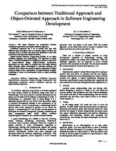
FIG. 1. Analytic vorticity for L 5 10D; units are arbitrary

analysis methods2 applied to the traditional scheme simply cannot obviate the principles shown theoretically in DC88. They may alter the quantitative outcome of the tests, but will not cause a qualitative change in the results. Second, the actual practice of objective analysis as applied to diagnoses based on observations [e.g., the widely used scheme developed by Koch et al. (1983)] is not significantly different from what we have chosen. Arguably, the biggest issue is whether or not to use a multiple-pass version of the traditional objective analysis method. We will demonstrate a potentially negative impact of multiple passes in what follows. We believe that our test is appropriate for helping those who employ the traditional scheme of derivative estimation to decide for themselves whether or not to consider switching to the line integral method for situations wherein derivatives are important to the diagnosis. As discussed in DC88, the two schemes both involve a mapping/smoothing operation and a derivative estimation operation. However, they differ in the order in which these two operations are performed. DC88 show that for irregularly distributed data, these operations do not commute; that is, the outcome necessarily involves different answers. It also is shown in DC88 that mapping/smoothing derivative estimates taken directly from 2 This statement assumes that the analysis is done with a globally uniform weighting function. That is, the unnormalized weight function is homogeneous. Inhomogeneous, anisotropic weight function shape parameters (as in Askelson et al. 2000) might provide a qualitative change in the characteristics of the traditional scheme with respect to derivative estimation, but are not in common use and have a number of issues associated with them (see Trapp and Doswell 2000).

VOLUME 129

FIG. 2. Delauney triangulation of the observing array perturbed using D s 5 0.8D. Triangles containing an included angle ,158 have been removed and are not considered in any analysis.

the observations is the ‘‘proper’’ order to perform the operations. a. The traditional scheme Our prototype scheme uses a simple, single-pass, distance-dependent weighted averaging scheme of the Barnes type (Barnes 1964). That is, it uses a Gaussian weighting of the form

OW f 5 , OW n

k

f˜ij

k

k51 n

(1)

k

k51

where ˜f ij denotes the value of the analyzed field at the Cartesian grid point (x i , y j ), n is the number of data points, f k is the value at the kth data point, and W k is the weight assigned to the kth data point. This weighting in (1) is given by W k 5 exp[2R k2 /l 2 ],

(2)

where R k2 5 (x i 2 x k ) 2 1 (y j 2 y k ) 2 in (2) is the Euclidean distance between the data point and the grid point in question. The parameter l determines the characteristics of the analysis; this is the ‘‘shape parameter’’ for the Gaussian weighting scheme. The weights for all data farther than 6l from a particular grid point are set to zero. Thus, the distance 6l represents a ‘‘cutoff radius’’ for the analysis scheme. For the horizontal wind field, the variables at the grid points will be the vector components(u˜, y˜ ).

OCTOBER 2001

For finite differencing, we employ the simplest possible scheme (one that is widely used in diagnostic practice, however), the centered, second-order scheme defined by

) d d )

] f˜ij d f˜ ø ]x dx ] f˜ij f˜ ø ]y y

ij

f˜ (x i11, y j ) 2 f˜ (x i21, y j ) (x i11 2 x i21 )

ij

f˜ (x i , y j11 ) 2 f˜ (x i , y j21 ) [ (y j11 2 y j21 )

[

) d d )

˜ ij 5 du˜ D dx u˜ x

1

ij

ij

2

) dy d )

dy˜ , dy ij

z˜ ij 5

˜ , y ij

d˜ shr | ij 5

) dy d )

dy˜ dx

(3)

˜ x

ij

) d d )

2

du˜ , dy ij

1

u˜ , y ij

ij

sponse of the scheme being determined by the choice of a weighting function and the parameters of the chosen scheme. 3. Description of the experiments

Observe that the differencing is done using the analyzed wind field, not the original data, which is characteristic of the traditional scheme. Once all four spatial derivatives are computed, the following quantities are determined from the finite-difference estimates of the wind vector component derivatives on the grid:

d˜ str | ij 5

2541

SPENCER AND DOSWELL

˜ ij , the analyzed where the analyzed divergence is D vorticity is z˜ ij , the analyzed stretching deformation is d˜ str | ij , and the analyzed shearing deformation is d˜ shr | ij . These are the four ‘‘kinematic’’ quantities that describe the linear (first order) characteristics of the wind field. They are more physically meaningful for wind field analysis than the four spatial derivatives; vorticity and divergence are commonly diagnosed from the wind field. b. The triangle scheme For the line integral method, we begin with a Delauney triangulation of the station network, as described in Ripley (1981, 39–41). In this application, any triangle created by this process with an included angle of less than 158 is omitted from consideration. Removing such narrow triangles from the analysis prevents potential problems with near-colinearity of the vertices. For each retained triangle, the four kinematic quantities of the wind field are computed using the LVPF method described in Zamora et al. (1987). This method assumes linearity of the wind field between the vertices of the triangles and assigns the calculated kinematic values to the triangle centroid. In order to plot the results, these quantities are treated as ‘‘data’’ located at the triangle centroids for an objective analysis using the same method as just given for the traditional scheme. Note that any objective analysis scheme using distance-dependent weighting will smooth the resulting analysis, to an extent that depends on the choice of the parameter(s) of the scheme (Stephens 1967). That is, in general, the schemes used for objective analysis behave as low-pass filters, with the amplitude and phase re-

Our goal is to determine quantitatively how well the two different prototypical methods estimate the derivatives of the wind field, as embodied in the four kinematic quantities. Since any test using real data necessarily means that we cannot know the ‘‘true’’ answer, we do not herein present any tests on real data. Rather, we follow the approach of Schaefer and Doswell (1979), using analytically specified input fields, but extend the tests to explore the sensitivity of the differences between the schemes to certain variables. The analysis grid is 161 3 161 grid points, where D g is the grid spacing (2.5 arbitrary units). The origin of the (x, y) coordinate system is at the center point of the analysis grid. The unperturbed data array comprises 441 observation sites in a 21 3 21 uniform array with grid spacing D (20 arbitrary units), such that D 5 8D g . The analysis grid has been chosen to be much finer than the data grid in order to minimize the effect of truncation error in finite differencing for waves detectable on the data array. a. Analytic data field structure Our wind component data are defined as functions of (x, y) at any point using a simple superposition of plane waves in the x and y directions:

1 L x2 sin1 L y2, 2p 2p y (x, y) 5 110 sin 1 x2 cos 1 y2, L L u(x, y) 5 210 cos

2p

2p

(4)

where the wavelength, which is an adjustable parameter, is given by L. The amplitude of the variation is 10 arbitrary units. This field is simply a ‘‘checkerboard’’ of cyclonic and anticyclonic vortices, so the analytic vorticity, which is given by

[

1 2 1 2 2p 2p 1 cos 1 x2 cos 1 y2 L L 2p 2p 2p 5 20 cos 1 x2 cos 1 y2, L L L

z (x, y) 5 10

2p 2p 2p cos x cos y L L L

]

is also a checkerboard of positive and negative vorticity centers (Fig. 1). Note that the amplitude of the vorticity increases as the wavelength decreases, which mimics

2542


FIG. 3. Vorticity estimates using (a) the traditional method, and (b) the triangle method, for L 5 10D, l 5 1.0D, and D s 5 0.8D.

the behavior of real velocity fields. Although we are not considering it, the analytic stretching deformation is d str (x, y) 5 20

1 2 1 2

2p 2p 2p sin x sin y . L L L

The other two kinematic quantities, divergence and shearing deformation, are identically zero for the analytic wind field.

VOLUME 129

FIG. 4. As in Fig. 3 except for L 5 25D and D s 5 0.2D.

b. Creation of artificial observing site arrays As already noted, we wish to know quantitatively the dependence of the improvements associated with the triangle method on the degree of irregularity of the observation site distribution, since DC88 suggested that it should increase as the irregularity increases. To accomplish this, we employ the methodology developed by Doswell and Lasher-Trapp (1997), whereby the location of each observation in an initially uniform array is ran-

OCTOBER 2001

SPENCER AND DOSWELL

2543

original unperturbed data array spacing. An example with D s 5 0.8D, a large value of irregularity, is shown in Fig. 2. c. Variables tested The variables we considered in our empirical testing were 1) D s , the scatter distance that measures the degree of irregularity in the observing site spacing; 2) l, the shape parameter for the objective analysis; and 3) L, the wavelength of the input analytic field. Our intent was to explore quantitatively the ideas developed theoretically in DC88, and to provide clear evidence for (or against) the implementation of the somewhat more complex line integral method of derivative estimation, instead of the traditional scheme. We also have considered the effect of fine and coarse analysis grids. 4. Results a. Pattern distortion results

FIG. 5. As in Fig. 3 except for L 5 25D. The data point locations are indicated by plus signs in (a) to show the relation between the vorticity maxima (peaks in the derivative field) and the data voids.

domly perturbed by a distance no greater than D s , the so-called scatter distance. A value of D s 5 0D implies the data distribution is uniform. Doswell and LasherTrapp showed that as D s increases, the data array becomes more irregular, up to a ‘‘saturation’’ value, beyond which there is no obvious increase in the irregularity of the distribution of stations. Saturation occurs when the value of D s is of roughly the same size as the

As a demonstration of the outcomes over what could be considered a typical application, consider Fig. 3. The wavelength of the input wave, L 5 10D, is more or less in the middle of the range identified as ‘‘marginally sampled’’ in DC88. Although the alternating pattern of positive and negative vorticity centers is captured by the traditional method, distortions of that pattern are quite evident (Fig. 3a). Extrema within the field are noticeably shifted from their true locations, with some being amplified relative to the analytic values, and large gradients are created in places where the true gradients should be relatively small. Close inspection reveals that these spurious gradients occur in relative data voids (caused by the irregularity of the data distribution), which agrees with the findings of Barnes (1994) and Spencer et al. (1999). This general finding also confirms those of Schaefer and Doswell (1979; see their Fig. 6 and accompanying discussion). On the other hand, the triangle method produces a pattern that is visually better than the traditional method (Fig. 3b). The gradients and locations of the extrema are analyzed much more faithfully with the triangle scheme, but it is noted that the peak values are somewhat reduced in comparison with those produced by the traditional method. Because the traditional method has amplified some of the peak derivative estimates beyond their true values, this general reduction in amplitude with respect to the traditional method is not necessarily a drawback of the triangle approach. A similar analysis for L 5 25D is done to represent a ‘‘well sampled’’ wave (according to DC88), with only a modest nonuniformity in the data array (D s 5 0.2D). This has a similar outcome (Fig. 4) to that with L 5 10D, which apparently contradicts the results shown in DC88’s Fig. 6. Their Fig. 6 was interpreted to suggest that for very long wavelengths, the difference in ‘‘fi-

2544


VOLUME 129

FIG. 6. Contour plot showing the difference (triangle minus traditional) of the rmse for vorticity between the triangle method and the traditional method, as a function of the shape parameter, l, and the wavelength, L, of the input analytic wave (as multiples of the data grid spacing, D) for (a) uniformly distributed data (D s 5 0.0D), (b) D s 5 0.5D, and (c) D s 5 1.0D. Negative values imply that the triangle method has lower rmse.

delity’’ between the traditional derivative estimates and the triangle method should become quite small. We will return to this point later. To complete this preliminary look at the results, we repeat the analysis for L 5 25D but with D s 5 0.8D again, a case of a highly irregular sample of a relatively long wave. Figure 5 demonstrates the extreme distortion of the field produced by the traditional method when compared to the triangle method (Fig. 5a), whereas for this situation, the triangle method has underestimated the amplitude of the peaks but again reproduces the pattern with considerable fidelity (Fig. 5b). Note the relationship between the peaks in the estimated vorticity and the data voids in Fig. 5a, even for a wave that is well-sampled by this data array.

b. Sensitivity to parameters As a way of summarizing the results of all the parameter sensitivity studies, we compute the root-meansquare error (rmse) as the difference between the analyzed and the true vorticity, where

O (z



rmse 5



 



ij

ij

2 z˜ ij ) 2 1/2

N

 



,

and where N is the number of grid points over which the rmse is computed. The calculation of rmse is done only over the interior part (i.e., the center 81 3 81 array) of the analysis grid, to avoid contamination of this statistic by boundary errors in the analysis (see Pauley

OCTOBER 2001

2545

SPENCER AND DOSWELL

the scattering approaches ‘‘saturation,’’ the value of d n gets smaller, owing to clustering. However, the total number of observations remains the same, so the reduction in d n does not represent an improvement in the data spacing, in terms of the fidelity with which the data can represent an input wave of some wavelength L . d n . It would be seriously misleading to believe that the sampling improves as its nonuniformity increases! An improved representation of the data spacing in nonuniform data arrays is that recommended by Koch et al. (1983): D nr 5 A1/2 FIG. 7. Box and whisker plot of the distance to the nearest neighbor as a function of D s , the scatter distance used to create nonuniform data distributions.

1990). This measure of the goodness of the fit has some limitations, but it is considerably more meaningful than computing the rmse at the data point locations (Glahn 1987). Figure 6a shows that, for uniformly distributed data, there is very little difference between the two methods except for l , 1.0D and for wavelengths below that considered to be marginally sampled. As discussed in Pauley and Wu (1990), there is very little reason ever to use a shape parameter that small, since it results in a serious overfitting of the data. Hence, it appears that there is no obvious benefit to the triangle method for uniformly distributed data, a result to be expected from the findings in DC88. However, when the data are moderately nonuniform (Fig. 6b), using values of 1.0D , l , 1.5D [i.e., values of l recommended by Pauley and Wu (1990)] results in some improvement by the triangle method for wavelengths greater than about L 5 11D. For a ‘‘saturated’’ nonuniform distribution of data (Fig. 6c), the triangle method yields lower rmse even when using a relatively ‘‘tight’’ fit (l 5 1.0D) for wavelengths greater than about L 5 7D, which is in the marginally sampled range. Again, these results suggest that it is for the longer wavelengths that the greatest benefit to using the triangle method is found. This is not the result expected in DC88, as noted. c. An issue tied to nonuniformity Before we discuss the reasons for this, however, it is useful to consider another aspect of the experiments, discovered during the experimental design. For many purposes, authors have used the average distance to the nearest neighbor (denoted here as d n ) as a way to characterize the ‘‘data spacing’’ of nonuniform arrays. Since Pauley and Wu (1990), inter alia, have made some specific recommendations about how to choose the shape parameter based on the average data spacing, this is worthy of some consideration. Figure 7 shows that as

1 M 2 1 2, 1 1 M 1/2

where M is the number of observations and A is the area within which the data are distributed. For large M, this reduces to D nr ø

12 A M

1/2

.

Thus, D n r represents the data spacing that would result if the data within the area A were uniformly distributed. Since we already knew the initial, unperturbed data spacing in our experiments, this is the parameter we used. Strictly speaking, even this is inappropriate, since nonuniform sampling increases the effective data spacing over that associated with a uniform distribution, as discussed in DC88 and recently considered by Trapp and Doswell (2000). d. Origins of the improvement over the traditional scheme at long wavelengths In DC88, it is suggested that ‘‘for wavelengths longer than 12Dx, the data can be considered continuous for many practical purposes, and finite difference derivative estimates will be accurate to within five percent . . . .’’ Our results do not show this. Instead it seems that even for very long waves, considerable distortion of the diagnosed derivative fields results from using the traditional method. By doing a series of traditional analyses with different values of l (not shown) during the initial mapping of the (u k , y k ) data onto the grid to derive the fields, it is possible to filter most of the ‘‘noise’’ from the traditional estimates of the derivative fields (e.g., the vorticity). The results of this experiment are summarized in Fig. 8, which shows that as the data become increasingly nonuniform, the minimum rmse associated with the traditional scheme occurs with increasing values of l, that is, with more smoothing. Figure 8 also shows that the slope of the axis of minimum rmse for the traditional method increases as the wavelength of the input wave increases. Increased smoothing implies that the amplitude of the field is reduced relative to that with less smoothing. It turns out that the production of a pattern comparable to that derived from the line integral method

2546


VOLUME 129

FIG. 8. Contours of the logarithm of the rmse associated with the traditional technique, as a function of shape parameter, l, and the scatter distance, D s , for an input wavelength, L, of (a) 8D, (b) 16D, and (c) 30D. The heavy line denotes the axis of minimum rmse.

via this heavy initial smoothing of the analyzed winds reduces the amplitude of the traditional method result even more than the amplitude reduction by the triangle scheme. A heavy initial smoothing in the traditional method can produce an improved pattern, but only at the cost of significant amplitude loss across the spectrum. On occasion, studies involving the diagnosis of derivatives using the traditional method employ a postoperative filter to remove the resulting noise (as exemplified by Fig. 3a) in the derivatives.3 We tested this 3 In some cases, a digital filtering is done to the analyzed fields (i.e., on the analysis grid) prior to estimating the derivatives. We have not considered this case, since it would be roughly equivalent to choosing a larger shape parameter for the initial mapping/smoothing operation.

by applying a simple five-point digital filter, with a spectral response function shown in Fig. 9, to the gridded derivative estimates of the traditional scheme. A single pass of this filter through the derivative estimates from the traditional method produced no apparent change in the derivative field (not shown). There is a simple reason for this: observe that our 161 3 161 analysis grid is considerably denser (by a factor of 8) than the data array. This means that reduction of the amplitude of 2D waves (i.e., on the data array, which would be 16 grid lengths on the analysis grid) to negligible levels (say, to 1% of their initial amplitude) would require many passes of this digital filter. Reduction of the 2D wave amplitude in this fashion to a low level necessarily results in a large loss of amplitude that would extend across the whole spectrum. If a coarser analysis grid than the one

OCTOBER 2001

SPENCER AND DOSWELL

FIG. 9. (a) Schematic of the simple five-point smoother, with (b) its associated response function as a function of the wavelength, in multiples of the grid distance D g .

we used is chosen to try to get around this problem, the consequence is an increased spatial truncation error during the finite-differencing step of the traditional scheme, not an attractive option. Hence, it seems that adding a postoperative filter to the traditional scheme does not appear capable of producing results comparable to the triangle method and cannot account for the discrepancy we are trying to resolve. Additional discussion of how the relative coarseness of the data and analysis grids affects the resulting analyses can be found in appendix A. The difference in the order of smoothing between the methods is not the direct source of the discrepancy, since the effect of asymmetric smoothing is negligible when the data are uniformly distributed (cf.

2547

FIG. 10. Plot of the traditionally computed (solid line) and true (dashed line) values along the row j 5 81 in the analysis grid for (a) the analyzed wind component, y˜ , and (b) the finite-difference form of the derivative [dy˜ ij /dx], using L 5 25D, D s 5 0.0D, and l 5 0.5D. The inset in (a) gives a slightly expanded view, for clarity.

Fig. 6). However, the difference in results between the methods is indeed related to way the smoothing is done, as we show below. In our experiments, the derivative estimates using the traditional method are particularly inferior at long wavelengths when a relatively small shape parameter, l, is used to fit the data relatively closely, even with uniform data spacing (cf. Fig. 6a). For large l, the differences between the methods are minor, but for small l (and, in particular, for 1.0D , l , 1.5D, where the objective analysis is being done properly), the traditional method is somewhat inferior. This suggests that the superiority

2548


of the triangle method over the traditional scheme might be associated with a type of overfitting of the data. We can illuminate this with the following somewhat exaggerated experiment. For L 5 25D, and D s 5 0.0D, we choose l 5 0.5D, and apply the traditional analysis to the data. The result is shown in Fig. 10a. What can be seen is that by deliberately overfitting the data, a small ‘‘plateau’’ is created in the vicinity of each data point; this is an artifact of the tightly fitted analysis. This feature creates a discontinuity in the gradient because, in the region near a data point, the extremely high weight given to that single datum (relative to any other data) is detrimentally influential on the resulting analysis. Therefore, in this case of extreme overfitting of the data, any differences between the values at nearby data points are obviously forced into the gap between sample points. Recall that this crowding of gradients into the voids between data points is characteristic of our results, even when not so exaggerated by the intentional overfitting. Therefore, even in the extreme case of a uniform data distribution, subsequent finite differencing creates obvious ‘‘spikes’’ in the derivative field (Fig. 10b). These effects can be removed by various artifices, such as a heavier initial smoothing, but we have shown that the results are generally inferior to those using the triangle method. 5. Discussion of results For most reasonable values of the shape parameter, l, it is clear that the traditional method produces markedly inferior estimates of the derivative fields when compared to the triangle method.4 Contrary to expectations expressed in DC88, this difference is not mitigated for features with well-sampled wavelengths. Rather, it is precisely in the long input wavelengths where the improvements obtained by using the triangle method are greatest. Hence, if the goal of doing an objective analysis is to diagnose derivatives with as much accuracy as possible, then there seems little alternative to doing the derivative estimates via the triangle (i.e., line integral) methods. There does not seem to be any simple way to create derivative estimates via the traditional method that compare favorably, under most realistic conditions, to those derived by the triangle approach. We tried a heavier initial smoothing and a postoperative digital filter to attempt to improve on the results using the traditional scheme, but found that neither of these changes gave derivative estimates as good as those obtainable via the triangle scheme. We recognize that our results call into question a rather substantial body of existing work involving derivative estimates, in view of the widespread use of the tradi4 We emphasize that the results shown thus far are for error-free, analytic observations. For a treatment of the impact of observation errors on the results, see appendix B.

VOLUME 129

tional method in diagnostic studies. We also realize that performing the line integral analysis involves more effort: a triangulation of the data points is needed, and line integrals need to be computed, rather than finite differences. Further, no common existing software can do the evaluations in this fashion. Until such software is made generally available, those wishing to do diagnosis involving derivatives will have to write their own software for the triangle approach. Nevertheless, the results of our experiments make it clear that using available software to estimate derivatives using the traditional method is done at some considerable peril to the accuracy of the calculations. Generally speaking, objective analysis of meteorological data for diagnostic purposes is done with the tightest fit to the data that gives acceptable results, in order to preserve the amplitude of the input field. When doing this with the traditional method, unfortunately, the resulting fields have distorted patterns, owing to the traditional method’s inherent inability to reproduce extrema and gradients accurately when doing a close fit to the data. We note that multiple-pass objective analysis schemes (i.e., those involving successive corrections, rather than just a single-pass mapping of the data from the irregular station distribution to a regular grid) generally will exaggerate this tendency for localized overfitting of the fields in the vicinity of the observation sites. Hence, it is not clear that multiple-pass objective analysis schemes can be given high recommendations if derivative estimates are the goal of the diagnosis. The traditional method produces inferior results even in situations with uniform spacing and long input wavelengths if the analysis is done with a relatively tight fit to the input data. As the data distribution becomes increasingly nonuniform, the traditional method’s inferiority to the triangle method is even more obvious. Given that virtually all routine observational networks (and even most experimental networks) have at least some degree of nonuniformity, it is not clear that using the traditional method should be the default choice for derivative estimation, in spite of its acceptance and common use in diagnostic studies. We hope that this set of experiments provides motivation for others to give serious consideration to changing their diagnostic derivative estimation methodology. Acknowledgments. We appreciate the very helpful comments concerning an early version of this manuscript from Mark Askelson and Jeff Trapp. We also acknowledge several helpful discussions on this general topic with Sonia Lasher-Trapp. Dave Watson provided us with considerable assistance in developing the Delauney triangulation algorithm, without which none of this would have been feasible. Finally, we thank the two anonymous reviewers, whose comments helped us clarify and improve the manuscript.

OCTOBER 2001

SPENCER AND DOSWELL

2549

FIG. A1. Estimated vorticity field with a uniform (D s 5 0) 21 3 21 data array, 161 3 161 analysis grid, for L 5 10D, l 5 1.0D, using the (a) traditional scheme, (b) the alternative scheme, and (c) the triangle scheme.

APPENDIX A A Simple Test of DC88 Theory According to the theory developed in DC88, the separate processes of estimating the derivatives and mapping/smoothing the field onto a uniform grid only commute when the data array coincides with the analysis grid. In cases where the data are on a uniform grid, it is possible to estimate the derivatives first, using (3) directly on the data array, and then mapping/smoothing the estimates onto the analysis grid. This procedure, which can

be carried out only in the case of a uniform data array, is called the alternative procedure, to distinguish it from the ‘‘traditional’’ and ‘‘triangle’’ schemes. In order to test this, we considered four separate experiments. First, we considered the 21 3 21 data array unperturbed from its original uniform arrangement, analyzing the result onto the 161 3 161 analysis grid using l 5 1.0D. The analytic field for L 5 10D (cf. Fig. 1) can be compared to the results shown in Fig. A1. All three methods give good results with respect to the pattern. The resulting amplitudes vary among the three different

2550


VOLUME 129

FIG. A2. As in Fig. A1 except for a 21 3 21 analysis grid that coincides with the data array.

schemes, but the traditional scheme retains the highest fraction of the amplitude. Second, we left everything the same except for reducing the size of the analysis grid to the same size as the data array and aligning the data array with the analysis grid. Results (Fig. A2) make it clear that the outcomes of the traditional and alternative schemes are virtually identical in this case, including the amplitudes. This seems to confirm the notion developed in DC88 that the processes of differentiation and smoothing do indeed commute when the data and

analysis grids coincide. The triangle scheme is also very similar to the other two, but it retains slightly more of the amplitude. Third, we repeated the experiment with the 21 3 21 data array unperturbed from its original uniform arrangement, analyzing the result onto the 161 3 161 analysis grid, but reduced the shape parameter to l 5 0.5D. That is, we deliberately ‘‘overfitted’’ the data. As can be seen in Fig. A3, the resulting analyses show that the traditional method fails to produce a good estimated derivative field, even with uniformly distributed data.

OCTOBER 2001

SPENCER AND DOSWELL

2551

FIG. A3. As in Fig. A1 except for l 5 0.5D.

The alternative scheme is much improved, although it apparently is suffering from substantial truncation error, as would be expected with such a coarse grid. The triangle method exhibits a slightly reduced amplitude compared to the alternative scheme in this case. Fourth, keeping l 5 0.5D, we repeated the experiment where the analysis grid and data array coincide exactly (Fig. A4). In this case, the traditional scheme actually produces a better field pattern than with a fine analysis grid. As with the previous example, the traditional and alternative schemes give virtually identical results, and the triangle scheme is very similar, only this

time it seems to retain slightly less amplitude than either of the other schemes. In the generally unrealistic situation of a uniform data array, our results confirm the theory developed in DC88. That is, the traditional and alternative schemes give virtually identical results when the data and analysis grids coincide. Interestingly, in this situation, the triangle scheme also gives similar but not quite identical results. By using line integrals to estimate the derivatives, the triangle method is doing something different, but we are not prepared to give a complete analysis of the process in comparison to the traditional approach.

2552


VOLUME 129

FIG. A4. As in Fig. A3 except for a 21 3 21 analysis grid that coincides with the data array.

APPENDIX B The Effect of Random Errors on Traditional and Triangle Calculations We now introduce random errors into the analytic wind field (4) in order to assess their impact upon the resulting traditional and triangle vorticity analyses. To do this, each component of every wind ‘‘observation’’ within the data array is assigned a different random error, generated by multiplying random num-

bers (between 61, drawn from a uniform distribution) by a value REmax , the maximum allowable random error. The random errors are then added to the analytic wind components and the analyses are performed. Here, REmax is varied from 0 to 10 m s 21 , the maximum wind amplitude [see Eq. (4)], for various combinations of the scatter distance (D s ) and wavelength (L). This provides a series of analyses. Sample results are presented in Fig. B1, which shows how the vorticity rmse varies with increasing random error for

OCTOBER 2001

SPENCER AND DOSWELL

2553

FIG. B2. Contour plot of the crossover point for various values of the scatter distance D s and the wavelength L. See text for details.

FIG. B1. Rmse for vorticity as a function of REmax , the maximum random error, for (a) D s 5 0.0D, L 5 10D and (b) D s 5 0.8D, L 5 10D. The solid curve is the rmse for the traditional method and the dashed curve is for the triangle method. Rmse values have been scaled by 10 5 .

particular values of D s and L. For all analyses presented on this appendix, l 5 1.0D. Figure B1a suggests that for REmax , 4 m s 21 , the traditional method is superior to the triangle method for the given values of D s and L, whereas the triangle method is superior for larger values of REmax. We emphasize that the traditional method is superior in the rmse sense for small values of REmax because it is better able to capture the true amplitude of the wave, although the patterns are very comparable. For example, compare

Figs. A1a,c to the corresponding analytic vorticity shown in Fig. 1. The value of REmax at which the two curves intersect is defined as the crossover point (COP). The COP is assigned a negative value if the traditional method vorticity rmse is lower than that of the triangle method for REmax , COP. Thus, for Fig. B1a, COP 5 24 m s 21 . For a more irregular data distribution (D s 5 0.8D), the triangle method is superior to the traditional method for REmax , 3 m s 21 (COP 5 13 m s 21 ; Fig. B1b). For example, Figs. 3a,b show that the pattern of the vorticity analysis is much superior for the triangle method than for the traditional analysis, although the traditional method appears to represent the magnitudes of the extrema more faithfully. A contour field of the COPs for various combinations of the scatter distance and wavelength is presented in Fig. B2. Interpretation of this figure is best done by example. For D s 5 0.0D and L 5 10D, the COP is estimated to be 24 m s 21 , which indicates that the traditional method rmse is lower than that for the triangle method for REmax , 4 m s 21 . This is consistent with the interpretation of Fig. B1a, as it should be. As another example, consider D s 5 0.8D and L 5 10D. For these values of scatter distance and wavelength, the COP is estimated to be 3 m s 21 , indicating that the triangle method rmse is lower than that for the traditional method for REmax , 3 m s 21 , a result consistent with the interpretation of Fig. B1b. Large, positive values of COP suggest that the triangle method rmse is smaller than the traditional method rmse over a large range of REmax , whereas the opposite is true for large, negative values of COP. From Fig. B2, we make three primary observations.

2554


First, for most wavelengths within and below the ‘‘marginally sampled’’ range (6D , L , 12D, as defined by DC88), the traditional method rmse is lower than the triangle method rmse for all degrees of data irregularity. Again, this is because the traditional method is better able to represent the true amplitude of the waves. For irregular data distributions (D s ± 0.0D), however, we have seen that despite having a larger rmse, the triangle method produces a superior pattern of the vorticity field. Second, for a perfectly regular data distribution (D s 5 0.0D) and for wavelengths exceeding the marginally sampled range, the COPs are very nearly zero, suggesting that the two methods are roughly equivalent. This result is consistent with our previous findings (e.g., Fig. 6a). Finally, for irregular data distributions—those found in real-life observational networks—and wavelengths greater than those considered marginally sampled, the triangle method is superior over a large range of REmax . In fact, even for only slightly irregular data distributions (0.1D , D s , 0.4 D), the triangle method generally is superior for values of REmax up to 4 m s 21 , errors greater than what would be expected from typical real observations. REFERENCES Askelson, M. A., J. P. Aubagnac, and J. M. Straka, 2000: An adaptation of the Barnes filter applied to the objective analysis of radar data. Mon. Wea. Rev., 128, 3050–3082. Barnes, S. L., 1964: A technique for maximizing details in numerical weather map analysis. J. Appl. Meteor., 3, 396–409. ——, 1994: Applications of the Barnes objective analysis scheme. Part I: Effects of undersampling, wave position, and station randomness. J. Atmos. Oceanic Technol., 611, 1433–1448. Bellamy, J. C., 1949: Objective calculations of vorticity, vertical velocity, and divergence. Bull. Amer. Meteor. Soc., 30, 45–50. Caracena, F., 1987: Analytic approximation of discrete field samples

VOLUME 129

with weighted sums and the gridless computation of field derivatives. J. Atmos. Sci., 44, 3753–3768. Ceselski, B. F., and L. L. Sapp, 1975: Objective wind field analysis using line integrals. Mon. Wea. Rev., 103, 89–100. Daley, R., 1991: Atmospheric Data Analysis. Cambridge University Press, 457 pp. Davies-Jones, R., 1993: Useful formulas for computing divergence, vorticity, and their errors from three or more stations. Mon. Wea. Rev., 121, 713–725. Doswell, C. A., III, and F. Caracena, 1988: Derivative estimation from marginally sampled vector point functions. J. Atmos. Sci., 45, 242–253. ——, and S. Lasher-Trapp, 1997: On measuring the degree of irregularity in an observing network. J. Atmos. Oceanic Technol., 14, 120–132. Glahn, H. R., 1987: Comments on ‘‘Error determination of a successive correction type objective analysis scheme.’’ J. Atmos. Oceanic Technol., 4, 348–350. Koch, S. E., M. des Jardin, and P. J. Kocin, 1983: An interactive Barnes objective map analysis scheme for use with satellite and conventional data. J. Climate Appl. Meteor., 22, 1487–1503. Pauley, P. M., 1990: On the evaluation of boundary errors in the Barnes objective analysis scheme. Mon. Wea. Rev., 118, 1203– 1210. ——, and X. Wu, 1990: The theoretical, discrete, and actual response of the Barnes objective analysis scheme for one- and two-dimensional fields. Mon. Wea. Rev., 118, 1145–1163. Ripley, B. D., 1981: Spatial Statistics. Wiley-Interscience, 252 pp. Schaefer, J. T., and C. A. Doswell III, 1979: On the interpolation of a vector field. Mon. Wea. Rev., 107, 458–476. Spencer, P. L., P. R. Janish, and C. A. Doswell III, 1999: A fourdimensional objective analysis scheme and multitriangle technique for wind profiler data. Mon. Wea. Rev., 127, 279–291. Steinacker, R., C. Ha¨berli, and W. Po¨ttschacher, 2000: A transparent method for the analysis and quality evaluation of irregularly distributed and noisy observational data. Mon. Wea. Rev., 128, 2303–2316. Stephens, J. J., 1967: Filtering responses of selected distance-dependent weight functions. Mon. Wea. Rev., 95, 45–46. Trapp, R. J., and C. A. Doswell III, 2000: Radar data objective analysis. J. Atmos. Oceanic Technol., 17, 105–120. Watson, D. F., 1992: Contouring: A Guide to the Analysis and Display of Spatial Data. Pergamon Press, 321 pp. Zamora, R. J., M. A. Shapiro, and C. A. Doswell III, 1987: The diagnosis of upper tropospheric divergence and ageostrophic wind using profiler wind observations. Mon. Wea. Rev., 115, 871–884.