A Quantitative Study of Texture Features across Different Window ...
Recommend Documents
Available online at www.sciencedirect.com. International Conference On ... aDepartment of Computer Science, Aberystwyth University, UK. bDepartment of ...
Sep 6, 2016 - R. Haralick, K. Shanmugam, I. Dinstein, Textural features for image classification, IEEE Transactions on Systems, Man and Cybernetics, 3.
Technological Educational Institute of Lamia. 3rd km Old ... Keywords: Image Analysis, Color Texture Features, Support Vector Machines. Reference to this ...
The opponent features are based on the opponent process theory of human color ... in color texture analysis, opponent features of LBP and Gabor wavelet ...
May 5, 2018 - the parameters of scale of the GLCM texture window greatly affecting ..... In theory, if one of the above frequency histograms shows an obvious ...
X-ray pole figure measmgments, the pole inclination, or, was changed from 5 to ... (o- fibre). 1 1 1> x,,. {011 ] ([3. -{0i i },i00 bre). 2=0. ,5 libre) t001 }.
welding. Then the foil is pushed down with a certain level of normal force by a roller-shaped ..... The authors also acknowledge Mark Norfolk (Fabrisonics,.
Supplementary Information. Quantitative ... Supplementary Information contains: ... Supplementary Figure S1| Evaluation and assessment of MS data quality.
Jan 2, 2013 - features and support vector machine for white blood cell ... Department of Computer Science & Software Engineering, Concordia University, ...
as Scalable TCP and HighSpeed TCP. We also relate window evolution under an AWP to workload process in queueing systems; this observation gives us a ...
pairwise comparisons between different image features, including MST versus average spectral texture ..... A. K. Jian. Fundamentals of Digital Image Processing.
Sep 21, 2015 - Department of Orthopedics, Huashan Hospital, Fudan University, Shanghai 200040, China .... using the SPSS12.0 (SPSS, Chicago, IL, USA). The indepen- ..... Hirayama disease,â Electroencephalography and Clinical Neuro-.
GLCM are andard Devia. MRI. Skull ull region ll stripped f K-means proach to .... M. Haralick, K. Shanmugam and I. Dinstein, "Textural Features for Image ...
Evaluation of Morphological Texture Features for Mangrove Forest Mapping and Species. Discrimination Using Multispectral. IKONOS Imagery. Xin Huang ...
Distinguishing Brazilian savanna physiognomies is an essential task to better evaluate carbon storage and potential emissions of greenhouse gases.
storage devices, scanning, networking, image compression, and desktop ... The typical application areas of such systems
Aug 31, 2007 - The power spectrum density (PSD) was estimated using Welch's .... The time series is converted to a symbolic sequence ..... the bootstrap. Boca.
Materials Science and Engineering, College of Engineering. Kittichai Sojiphan1, Sudarsanam Suresh Babu1,. X. Yu2, and S.C. Vogel2. 1Department of ...
Jun 30, 2016 - ... the excellent technical assistance of Montserrat Robledo and Anna .... Reynolds A, Lundblad V, Dorris D, Keaveney M. Yeast Vectors and ...
vamos uma diminuição do número e da densidade volumétrica dos lisosomos nos pinealócitos. Esses resultados mostram que a melatonina atua sobre a ...
Le trote fario hanno prodotto volumi minori (4,5 vs 18,13 ml) di sper- ma, ma ... Parole chiave: Pesci, Liquido seminale, Composizione acidi grassi, Motilità spermatica, Densità spermatica. .... rates was higher for RT (75 %) than for GSB (~15.
Keywords: Image classification; Image segmentation; Texture; Color; Gaussian mixture models; Expectation ... 1 By the word 'texture', we denote both what we will later call ..... classifications: there is a tendency for blocks near the center.
May 20, 2006 - acoustic features, such as Mel-Frequency Cepstral Co- efficient (MFCC) or ..... [3] S. B. Davis and P. Mermelstein, âComparison of. Parametric ...
A Quantitative Study of Texture Features across Different Window ...
Jul 25, 2016 - ... on the performance of prostate cancer CAD and to identify discriminant ... Understanding and Analysis Conference, MIUA15, Lincoln, UK, pp.
International Conference On Medical Imaging Understanding and Analysis 2016, MIUA 2016, 6-8 July 2016, Loughborough, UK
A Quantitative Study of Texture Features Across Different Window Sizes in Prostate T2-Weighted MRI Andrik Rampuna,∗, Liping Wanga , Paul Malcolmb , Reyer Zwiggelaara,∗ a Department b Department
of Computer Science, Aberystwyth University, UK of Radiology, Norfolk and Norwich University Hospital, UK
1. Introduction The ultimate goal of this study is to investigate the relationship between window size and image texture features for classification purpose in prostate T2-Weighted Magnetic Resonance Imaging (T2-W MRI). In the development of prostate cancer Computer Aided Diagnosis (CAD) systems, textures are among the most important elements in characterising different regions of the prostate. Most texture descriptors require a window to extract features. Unfortunately, none of the previous prostate cancer CAD studies have investigated the performance of their proposed methods when the same features are extracted using different window sizes (ws) as this process is time consuming and computationally expensive. Many studies selected ws based on the previous studies although the studies did not perform a quantitative evaluation on the selections of ws. As a result, the selection of ws in prostate cancer CAD in the literature vary significantly. For example, in the study of Niaf et al. 1 and Chan et al. 2 they used 9 × 9. On the other hand, Rampun et al. 3 suggested 9 × 9 and 11 × 11. The study of Viswanath et al. 4 used 5 × 5 and 7 × 7 depending on the types of features extracted whereas Ampeliotis et al. 5 and Ikonen et al. 6 used 3 × 3. Another issue in the development of prostate cancer CAD is the selection of texture descriptors in T2-W MRI. It is common that features were selected based on their performance in general texture classification and popularity. For ∗
instance, first and second order statistical features are among the most popular texture descriptors used to characterise regions in the prostate. On the other hand, filter-based (e.g. Gabor and Gaussian filters) and histogram-based (Local Binary Pattern and Textons) features can provide rich information about the texture. Since, there have been a limited number of studies that have attempted to identify the most discriminant features and the effects of the ws selection, in this study we conducted the following experiments: • We evaluated the effect of ws on the CAD and feature performance. In this study we selected 3 × 3, 5 × 5, 7 × 7, 9 × 9, 11 × 11, 13 × 13, 15 × 15, 17 × 17 and 19 × 19. • We extracted a set of 215 image features and identify the top 10 most discriminant features across different ws. • We evaluated the CAD performance using the top 10 features extracted using different ws. Based on the above experiments, the contributions of this study are two-fold: (a) This study gives a general guideline on ws selection in the development of prostate cancer CAD and (b) The identified top 10 features can be used as a starting point on the selection of texture descriptors in the prostate. 2. Overview of the CAD System
Fig. 1: A general overview of the CAD system
Following the study of Rampun et al. 3 , Figure 1 shows an overview of the CAD system used in this study. Firstly 215 image features were extracted from benign and malignant regions in the prostate T2-W MRI. To avoid absolute values playing a role in the feature selection stage each of the feature vectors was linearly scaled to the range [0,1] and the same was applied for the test data. Feature selection was performed to avoid over-fitting when building a classifier model as less data means less chance of making decisions based on noise. We employed the CfsSubsetEval 7 attribute evaluator and the GreedyStepwise search method in WEKA 8 . Firstly, the dataset was separated into training and testing sets (using 9-fold cross validation (9-FCV)) and we performed feature selection based on the training set only. Subsequently, we use the same selected features in the testing set. In the training and testing stage, we employed the Bayesian Network (BNet) and Random Forest (RF) classifiers in WEKA 8 (note that all parameters were left on default settings in WEKA 8 ). All pixels within the radiologists tumor annotation were extracted as prostate cancer samples. This area was truncated by the tumor mask, to ensure no pixels outside the tumor region were included into the malignant samples. On the other hand, every pixel outside the tumor region was considered as benign samples. Similarly, this region is truncated by the tumor and prostate gland masks to ensure no pixels within the tumor region and outside the prostate gland were included as benign samples. Only cancer regions within the prostate peripheral zone were considered. A stratified nine runs 9-fold cross validation scheme was employed. The evaluation was based at a patient level to ensure no samples from the same patient were used in the training and testing phases. Each classifier was trained and in the testing phase, each unseen instance/pixel from the testing data (taken from 5 randomly selected patients) was classified as malignant or non-malignant. 3. Materials and Dataset Our dataset consists of 418 T2-W MR images (227 malignant and 191 normal slices resulting in 74,208 malignant pixels and 97,310 normal pixels) taken from 45 patients aged 54 to 74. Each patient has between 6 to 13 slices covering the top to the bottom of the prostate gland. The prostate gland, malignant regions and transitional zone were delineated by an expert radiologist with more than 10 years experience in prostate MRI. All sequences with prostate cancer cases were confirmed malignancies based on TRUS biopsy reports and malignant regions annotated cases were clinically significant cancer (Gleason score grade 7 and above). All patients underwent T2-W MR imaging at the Department of Radiology at the Norfolk and Norwich University Hospital, Norwich, UK. MR acquisitions were performed prior
to radical prostatectomy. All images were obtained on a 1.5 Tesla magnet (Sigma, GE Medical Systems, Milwaukee, USA) using a phased array pelvic coil, with a 24 × 24 cm field of view, 512 × 512 matrix, 3mm slice thickness, and 3.5mm inter-slice gap. 4. Experimental Design
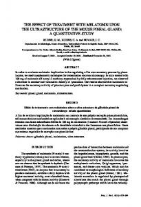
Fig. 2: A general overview of the experimental design
Figure 2 represents the overview of the experimental design used to assess the effects of ws on a CAD performance and to identify discriminant features among the 215 features extracted in this study. Note that the CAD system used in this study was summarised in Section 2 and details can be found in Rampun et al. 3 . Firstly, the system extracted features using different ws and fed them into the CAD system. In the CAD system, the CfsSubsetEval 7 attribute evaluator selects relevant features for training and testing. The process is repeated by feeding the CAD system with features extracted using ws = 3 × 3 to 19 × 19. All selected features in every iteration were recorded (e.g. selected features using 3 × 3, 5 × 5, etc.). Subsequently, we identified the top 10 common features (for simplicity) across different ws. Using these top 10 features (extracted using different ws), we train and test the BNet and RF classifiers to evaluate the effects on the systems performance. The classification contains two classes which are malignant (regions annotated by a radiologist based on the TRUS biopsy report) and non-malignant. 4.1. Summary of Texture Features The extracted image features were mainly motivated by statistical and image and signal processing points of view. These features were selected based on the visual characteristics of malignant regions as indicated by expert pathologists and radiologists as well as their efficiency at discriminating malignant and benign regions 9,13 . The first and second order statistical features, filter bank features, Tamura texture features and grey-level percentile based features estimated for each pixel for a local n × m window where n and m are rows and columns, respectively. Table 1 summarises the list of features used in this study which are divided into six categories. Table 1: Summary of features used in this study. Category F1 : F2 : F3 : F4 : F5 : F6 :
Features Mean, median, standard deviation, mean and median of absolute deviation, skewness, kurtosis, mean of correlation coefficients, local contrast, variance and local probability GLCM features of Haralick et al. 11 , Soh and Tsatsoulis 12 and Clausi and Deng 14 by taking 4 orientations and mean, variance and standard deviation of 4 orientations Grey-level percentile 25% and percentile 75% Tamura’s textures features namely coarseness, contrast and directionality Image numerical gradient (0◦ and 90◦ orientations), image magnitude, using Sobel operator image gradient (0◦ , 90◦ and diagonal orientations) and image magnitude. Filter bank of Varma and Zisserman 13 which contains an edge and a bar filter, at 6 orientations and 3 scales, a Gaussian and Laplacian of Gaussian filters
4.2. Feature Selection Since the CAD system employed 9-fold cross validation (dataset was separated into training and testing sets), the feature selection process was repeated 81 times (each fold has 9 runs). The entire process resulting a feature has a maximum of 81 selections (ns) (in each ws). The higher the ns the more frequently the feature has been selected by CfsSubsetEval 7 . By ranking the features based on their ns, the most discriminant feature is the one with the highest ns value. The entire process has a maximum ns of 729 (81 × 9 ws) that can be achieved by each feature. Furthermore, we identify the top 10 most common features (Fc f ) by calculating the total ns for each feature across different ws. 5. Experimental Results In this section we will present the most discriminant features from each ws, the common features across different ws, Area Under the Curve (Az ) which indicates the trade-off between the true positive against the false positive rate and finally classification accuracy (CA) which represents the number of pixels classified correctly. 5.1. Selected Features From Each ws Table 2: Summary of selected features with the high ns. Category 3×3 5×5
7×7 9×9 11 × 11 13 × 13 15 × 15 17 × 17 19 × 19
Features Gaussian filter, Laplacian of Gaussian filter and image magnitude (ns = 81),Standard deviation, GLCM: sum of squares variance (θ = 135◦ ), GLCM: variance of homogeneity (θ = 0◦ , 45◦ , 90◦ , 135◦ ) (ns=78), local probability, local contrast, median (ns=76) GLCM: sum of squares variance (θ = 135◦ ), Gaussian filter, Laplacian of Gaussian filter, bar/spot filter ((σ x , σy ) = (1, 3), θ = 30◦ ), bar/spot filter ((σ x , σy ) = (1, 3), θ = 0◦ ), edge filter ((σ x , σy ) = (1, 3), θ = 90◦ ), image magnitude, image magnitude of Sobel operator, variance (ns = 81), image gradient θ = 90◦ , image gradient θ = 0◦ (ns = 80), local probability, local contrast (ns = 79) Gaussian filter, Laplacian of Gaussian filter, bar/spot filter ((σ x , σy ) = (1, 3), θ = 0◦ ), bar/spot filter ((σ x , σy ) = (1, 3), θ = 90◦ ), image magnitude of Sobel operator, image magnitude, variance (ns = 81), bar/spot filter ((σ x , σy ) = (1, 3), θ = 30◦ ) (ns = 77), bar/spot filter ((σ x , σy ) = (1, 3), θ = 150◦ ) (ns = 74) Gaussian filter, Laplacian of Gaussian filter, bar/spot filter ((σ x , σy ) = (4, 12), θ = 0◦ ), image magnitude of Sobel operator, image gradient of Sobel operator (θ = 45◦ ), image magnitude, image gradient (θ = 90◦ ), Tamura contrast (ns = 81), Image gradient of Sobel operator (θ = 90◦ ), local probability (ns = 80), local contrast (ns = 79) Gaussian filter, Laplacian of Gaussian filter, image magnitude of Sobel operator, Tamura contrast, image magnitude , variance (ns = 81), bar/spot filter ((σ x , σy ) = (2, 6), = 0◦ ), local probability (ns = 70), bar/spot filter ((σ x , σy ) = (1, 3), = 90◦ ) (ns = 63), image gradient of Sobel operator (θ = 45◦ ) (ns = 54) GLCM: sum of squares variance (θ = 135◦ ), bar/spot filter ((σ x , σy ) = (1, 3), θ = 60◦ ), image gradient of Sobel operator (θ = 45◦ ), image magnitude, image gradient (θ = 90◦ ), Tamura contrast, variance and local contrast (ws = 13 × 13), image magnitude of Sobel operator and local probability (ns = 78) Image gradient of Sobel operator (θ = 45◦ ), image magnitude, image gradient (θ = 90◦ ), Tamura contrast, variance (ns = 80), image magnitude of Sobel operator and local probability (ns = 75) Variance, Tamura contrast, image gradient (θ = 0◦ ) (ns = 81), image magnitude of Sobel operator and image magnitude (ns = 77) Image gradient (θ = 0◦ ), image magnitude and Tamuras contrast (ns = 80), edge filter ((x , y ) = (1, 3), = 60 ), variance (ns = 70)
Total 65
64
59
62
63
60
58 55 54
Table 2 summarises the results of the most discriminant texture features and the total number of features selected (TF) out of 215 features in each ws. In our analysis the second order statistical features (F2 ) did not work well at most window sizes and were discriminant only when extracted using 3 × 3 or 5 × 5. On the other hand, the first order statistical features (F1 , F3 and F4 ) worked well when extracted using ws = 9 × 9 or 11 × 11. The gradient-based features and the filter bank are consistent in most ws. On the other hand, Table 3 and 4 summarise the performance of the CAD in both metrics. It should be noted that these results are based on the selected features by the CfsSubsetEval 7 method out of 215 image features. The results in Table 3 show that both classifiers achieved the best Az equal to 90% and 87.9% at ws = 11 × 11 with only 0.1% difference at ws = 9 × 9. The Az values for both classifiers are gradually
decreasing towards the largest and smallest ws. The trend is slightly different in Table 4 as the best CA = 88.1% was achieved at 13 × 13 of the BNet classifier. However, the RF classifier achieved the best CA at 9 × 9. Table 3: Az (%) values using different window sizes based on the selected features by CfsSubsetEval 7 . 3×3
5×5
7×7
9×9
11 × 11
13 × 13
15 × 15
17 × 17
19 × 19
BNet
85.7 ± 9.2
87.1 ± 9.8
88.1 ± 8.5
89.9 ± 9.9
90.0 ± 7.6
82.7 ± 9.9
83.1 ± 11.6
83.1 ± 13.3
82.3 ± 14.9
RF
83.2 ± 8.1
85.1 ± 8.6
85.7 ± 9.0
87.8 ± 9.2
87.9 ± 9.3
82.2 ± 9.8
82.2 ± 11.9
81.3 ± 12.7
76.8 ± 15.4
Table 4: CA (%) using different window sizes based on the selected features by CfsSubsetEval 7 . 3×3
5×5
7×7
9×9
11 × 11
13 × 13
15 × 15
17 × 17
19 × 19
BNet
80.3 ± 6.1
81.4 ± 6.4
82.2 ± 6.6
82.6 ± 8.3
83.5 ± 7.6
88.1 ± 9.8
87.3 ± 11.5
82.3 ± 11.7
81.3 ± 15.2
RF
81.3 ± 5.9
82.3 ± 5.6
82.7 ± 6.0
85.2 ± 5.3
84.7 ± 7.2
83.1 ± 12.9
81.2 ± 15.4
84.3 ± 15.4
79.6 ± 18.7
5.2. Top 10 Common Features Across Different ws In our analysis we found the following features are the most common across different ws together with their ns: Image magnitude (723), Image magnitude of Sobel operator (687), Local probability (668), Variance (623), Gaussian filter and Laplacian of Gaussian (616), Local contrast (601), Tamura contrast (543), Image gradient (θ = 0◦ ) (469) and Image gradient (θ = 90◦ ) (403). Following on from these findings, we re-ran the CAD system by feeding it using these top 10 common features (extracted using different ws) to evaluate the performance of the system. Table 5 and 6 summarise the performance of the CAD in both metrics when using the top 10 common features extracted using different ws. The results in Table 5 and 6 suggest that the BNet classifier still produced Az > 89% at 9 × 9 and 11 × 11 even after reducing the data dimension to 10. Using the top 10 common features across different ws still give the BNet classifier Az > 80% which is similar to the RF classifier (except the largest ws). In terms of CA, both classifiers achieved the highest accuracy at 9 × 9 which are 84.3% and 83.8% for the BNet and RF classifier, respectively. Table 5: Az (%) values using different window sizes based on the top 10 selected features. 3×3
5×5
7×7
9×9
11 × 11
13 × 13
15 × 15
17 × 17
19 × 19
BNet
83.5 ± 8.2
84.3 ± 8.3
85.8 ± 8.7
89.8 ± 7.7
89.1 ± 7.6
85.0 ± 12.7
83.8 ± 15.1
82.7 ± 14.1
81.2 ± 15.2
RF
80.4 ± 9.3
81.1 ± 7.5
83.6 ± 9.5
86.1 ± 9.5
86.4 ± 8.7
82.5 ± 11.5
83.4 ± 13.5
81.1 ± 13.7
78.1 ± 14.2
Table 6: CA (%) using different window sizes based on the top 10 selected features. 3×3
5×5
7×7
9×9
11 × 11
13 × 13
15 × 15
17 × 17
19 × 19
BNet
79.3 ± 6.3
80.1 ± 7.4
82.2 ± 6.8
84.3 ± 6.6
84.0 ± 8.5
81.5 ± 11.2
82.3 ± 9.2
80.5 ± 10.6
80.3 ± 14.2
RF
78.2 ± 6.5
79.5 ± 6.7
80.0 ± 6.5
83.8 ± 5.2
82.9 ± 7.4
80.4 ± 9.2
81.3 ± 11.1
80.3 ± 14.7
79.8 ± 17.9
6. Discussions and Conclusions The goal of this study is to investigate the effects of ws on the feature itself and the CAD performance as well as to identify a set of good texture descriptors in prostate T2-W MRI. Our experimental results suggest that the top 10 common features across ws can be used as a starting point in selecting texture features to distinguish malignant and normal regions in the development of CAD systems. This can be seen in Table 5 where the Az value is always
consistently above 80% across different ws using the same features. On the other hand, our experimental results suggest that the best ws is either 9 × 9 or 11 × 11. Our explanation for this are three-fold: firstly using a small ws such as 3 × 3 does not provide sufficient information about the regions (such as limited intensities and grey level variations). Secondly, using a medium ws (e.g. 9 × 9) features tend to be more reliable because noisy pixels are shrunk by the domination of reliable pixels (e.g. malignant pixels). Finally, when using a large ws (e.g. 19 × 19), the performance tends to decrease because the chance of mixing up pixels from benign and malignant class is higher, hence altering the actual features representation of a particular class. However, we are aware that the selection for the best ws and texture features might vary depending on various factors such as the image’s pixel size, the level of noise and the types of feature selection used. For instance, although 9 × 9 and 11 × 11 produced the best results, these may be different if an image with a larger or smaller pixel size was used. In our dataset the pixel size is 0.47mm (ws = 3 × 3 is equivalent to 1.41mm × 1.41mm). Moreover, the selection of ws has a significant effect on both metrics particularly when using a very small and large ws (e.g. 3 × 3 and 19 × 19). As presented in Table 3,4,5 and 6 the difference between the results using average ws and the smallest and largest ws is vary between 3% to 8%. In conclusion, we have conducted and presented our experimental results in this paper which suggest that a medium ws (e.g. 9 × 9 and 11 × 11) is a fair selection for an initial investigation in feature extraction and the top 10 common features could be used as a set of good descriptors in capturing texture characteristics in the prostate. Nevertheless, these findings might be inconsistent depending on the architecture of the CAD system and the types of texture features which could be investigated in our future work. References 1. Niaf E., Rouvi`ere O., e` ge-Lechevallier F.M., Bratan F., Lartizien C. Computer aided diagnosis of prostate cancer in the peripheral zone using multiparametric MRI. Physics in Medicine and Biology, vol. 57(12):3833–3851, 2012. 2. Chan I., Wells III W., Mulkern R.V., Haker S., Zhang J., Zou K.H., Maier S.E., Tempany C.M. Detection of prostate cancer by integration of line-scan diffusion, T2-mapping and T2-weighted magnetic resonance imaging; a multichannel statistical classifier. Medical Physics, vol.30(9):2390–2398, 2012. 3. Rampun A., Zheng L., Malcolm P., Zwiggelaar R. Computer Aided Diagnosis of Prostate Cancer within the Peripheral Zone in T2-Weighted MRI. In Proceedings of the 19th Medical Image Understanding and Analysis Conference, MIUA15, Lincoln, UK, pp. 207–212, July 2015. 4. Viswanath S.E., Bloch N. B., Chappelow J.C., Toth R., Rofsky N.M, Genega E.M., Lenkinski R.E., Madabhushi A. Central gland and peripheral zone prostate tumors have significantly different quantitative imaging signatures on 3 Tesla endorectal, invivo T2-weighted MR imagery. Journal of Magnetic Resonance Imaging, vol. 36(1):213–224, 2012. 5. Ampeliotis D., Antonakoudi A.,Berberidis K., Psarakis E.Z., Kounoudes A. A Computer-Aided System for the Detection of Prostate Cancer Based on Magnetic Resonance Image Analysis. In Proceedings of the 3rd International Symposium on Communications, Control and Signal Processing (ISCCSP 2008), March 12–14, 2008, Malta. 6. Ikonen S., Karkkainen P., Kivisaari L., Salo J.O., Taari K., Vehmas T., Tervahartiala P., Rannikko S. Magnetic resonance imaging of clinically localized prostatic cancer. Journal of Urology, vol. 159 (3), pp. 915–919, 1998. 7. Hall M.A. Correlation-based feature selection for discrete and numeric class machine learning. In Proceedings 17th International Conference of Machine Learning, pp. 359–366, 2000. 8. Hall M., Frank E., Holmes G., Pfahringer B., Reutemann P., Witten I.H. The weka data mining software: an update. ACM SIGKDD explorations newsletter, vol. 11(1):10–18, 2009. 9. Norberg M., Egevad L., Holmberg L., Sparen P., Norlen B.J., Busch C. The sextant protocol for ultrasound-guided core biopsies of the prostate underestimates the presence of cancer. Journal of Urology, vol. 50(4):562–566, 1997. 10. Plewes D.B., Kucharczyk W. Physics of MRI: a primer. Journal of Magnetic Resonance Imaging, vol. 5(35):1038–1054, 2012. 11. Haralick R.M., Shanmugam K., Dinstein I. Textural features of image classification. IEEE Transactions on Systems, Man and Cybernetics, vol. 3(6):610–621, 1973. 12. Soh L., Tsatsoulis C. Texture analysis of sar sea ice imagery using gray level co-occurrence matrices. IEEE Transactions on Geoscience and Remote Sensing, vol. 37(2):780–795, 1999. 13. Varma M., Zisserman A. A statistical approach to texture classification from single images. International Journal of Computer Vision, vol.62:61–81, 2005. 14. Clausi D.A., Deng H. Design-based texture feature fusion using gabor filters and co-occurrence probabilities. IEEE Transactions on Image Processing, vol. 14(7):925–936, 2005.