A Randomized O(m log m) Time Algorithm for Computing Reeb Graphs of Arbitrary Simplicial Complexes William Harvey∗ , Yusu Wang∗ and Rephael Wenger∗
Abstract Given a continuous scalar field f : X → IR where X is a topological space, a level set of f is a set {x ∈ X : f (x) = α} for some value α ∈ IR. The level sets of f can be subdivided into connected components. As α changes continuously, the connected components in the level sets appear, disappear, split and merge. The Reeb graph of f encodes these changes in connected components of level sets. It provides a simple yet meaningful abstraction of the input domain. As such, it has been used in a range of applications in fields such as graphics and scientific visualization. In this paper, we present the first sub-quadratic algorithm to compute the Reeb graph for a function on an arbitrary simplicial complex K. Our algorithm is randomized with an expected running time O(m log n), where m is the size of the 2-skeleton of K (i.e, total number of vertices, edges and triangles), and n is the number of vertices. This presents a significant improvement over the previous Θ(mn) time complexity for arbitrary complex, matches (although in expectation only) the best known result for the special case of 2-manifolds, and is faster than current algorithms for any other special cases (e.g, 3manifolds). Our algorithm is also very simple to implement. Preliminary experimental results show that it performs well in practice.
∗
Computer Science and Engineering Department, The Ohio State University, Columbus, OH 43210. harvey,yusu,
[email protected]
Emails:
1
Introduction
Let f : X → IR be a continuous function defined on a topological space X. For each scalar value α ∈ IR, the set {x ∈ X : f (x) = α} is called a level set of f . A level set of f can be partitioned into connected components. The Reeb graph of f is obtained by continuously collapsing every component of each level set into a single point. As α increases, connected components appear, disappear, split and merge, and the Reeb graph of f tracks such changes. The mathematical concept of the Reeb graph was first defined by George Reeb [19] for smooth manifolds. It was introduced in graphics applications by Shinagawa et al. [22]. Since then, it has been used in a range of shape analysis applications, including shape understanding [2, 3, 22], segmentation and matching [14, 20, 25, 27], shape repairing and animation [15, 29], surface quadrangulations and parametrization [13, 18, 30]. See [4] for a very nice survey paper on the Reeb graph and its applications. The loop-free version of the Reeb graph, commonly known as the contour tree, is also a popular tool for analyzing scalar fields [5], and has a long history in fields such as geographic information systems and scientific visualization. In all these applications, it is important to be able to construct the Reeb graph in an efficient manner. We consider the problem of computing Reeb graphs of f : X → IR, where f is a piecewise linear function defined on a simplicial complex X. A straightforward approach to computing the Reeb graph is to track the connected components of the level sets and update the Reeb graph as the components change. While this approach is conceptually simple, it can be tricky to implement. Moreover, on a 2-complex with n vertices and m triangles, this approach can take Θ(mn) time. Our contribution. As discussed in Section 2, a number of papers present efficient algorithms for computing Reeb graphs in special cases, such as when X is a two or three manifold. This paper describes an efficient randomized algorithm for arbitrary simplicial complexes. The algorithm runs in O(m log n) expected time, where m is the number of 0, 1, and 2-simplices in the complex and n is the number of vertices. Specifically, for a point q ∈ X, let Lq be the level set {x ∈ X : f (x) = f (q)} and let Cq be the connected component of Lq which contains q. Our algorithm picks a random vertex q in the complex and “collapses” all the triangles intersecting Cq onto q and its adjacent edges. The algorithm then picks another random vertex and repeats this collapse procedure. New triangles will be created and collapsed during the process, and the expected total number of these intermediate triangles is O(m log n). As a result, the expected running time of our algorithm is also O(m log n). Our contributions are as follows: • We give the first sub-quadratic time algorithm for an arbitrary simplicial complex. Our expected running time matches the running time of the best current algorithm for 2-manifolds (although only in expectation) and is faster than any other current algorithm. • Our algorithm and its implementation are very simple. The implementation uses a repetition of just one “collapse” operation, and involves only array and linked-list data structures. • We show preliminary experimental results to demonstrate the practical potential of our algorithm.
2
Related work
In [6], Carr et al. presented a simple and efficient algorithm to compute the contour tree of an arbitrary simplicial complex domain X in O(n log n + mα(m)) time, where n is the number of vertices in the input simplicial complex and m is the size of its 2-skeleton (i.e, the total number of vertices, edges and triangles). The algorithm improved ideas from several previous contour-tree algorithms [24, 28]. Shinagawa and Kunii presented the first provably correct algorithm to compute Reeb Graphs for a triangulation of a 2-manifold [21]. Their algorithm runs in Θ(n2 ) time. It sweeps vertices of the mesh in 1
References [7] [10]
[9] [26] [17]
Underlying Domain 2-manifolds 3-manifolds 3-manifolds d-manifolds 3-manifolds arbitrary simplicial complex 3-manifolds embedded in IR3 arbitrary simplicial complex
Time Complexity O(n log n) = O(m log m) O(m log m + m log g(log log g)3 ) O(mg log2 m) (implemented algorithm) O(m log m(log log m)3 ) O(m log m + L) = Θ(mn) O(mn) O(m log m + hm) = Θ(mn) O(mn)
Table 1: Current best algorithms to compute Reeb graph for a simplicial complex X. m is the size of the 2-skeleton of X (i.e, total number of vertices, edges and triangles), and n is the number of vertices.
increasing order of function values, and maintains the level-sets explicitly during the sweeping. This sweeping idea can be used to compute the Reeb graph for arbitrary simplicial complex in Θ(nm) time. Since then, there have been several more efficient algorithms, mainly focusing on 2 or 3-manifolds. We summarize the results in Table 2 and briefly review them below. For the case of 2-manifold, Cole-McLaughlin et al. [7] improved the running time from O(n2 ) to O(n log n) based on their insights in the structure of the level sets and Reeb graph for 2-manifolds. Doraiswamy and Natarajan [10] further extended the sweeping idea to handle 3-manifolds, and presented an O(m log m + m log g(log log g)3 ) time algorithm, where g is the maximum genus of any iso-surface. Their algorithm uses dynamic spanning tree / co-trees to maintain connectivity of level sets during the sweeping. It can be extended to d-manifolds (by using a fully-dynamic graph connectivity algorithm) with a running time O(m log m(log log m)3 ). They also provided a simpler but slower implementation that runs in O(mg log2 m) time to compute the Reeb graph for functions on 3-manifolds. An interesting and simple semi-output sensitive algorithm is proposed in [9] to compute the Reeb graph of 3-manifolds in time O(m log m + L), where L is the total complexity of all level-sets passing through critical points and can be Θ(nm) in worst case. The same algorithm can handle arbitrary simplicial complexes, but the bound of O(m log m + L) will then not hold. Very recently in [26], Tierny et al. proposed an algorithm that computes the Reeb graph for a 3-manifold with boundary embedded in IR3 in time O(m log m + hm), where h is number of independent loops in the Reeb graph. Their approach leverages the efficient contour tree algorithm in [5] by using a novel surgery idea to first cut the input simplicial complex so that its Reeb graph is loop-free. The worst case time complexity can be Θ(nm), but it runs much faster in practice as h is usually small. Finally, a streaming algorithm was presented in [17] to compute the Reeb graph for an arbitrary simplicial complex in Θ(nm) time. Reeb graphs for time-varying functions defined on 3-dimensional domains was studied in [12] exploiting Jacobi sets. In the field of graphics, there are also several practical implementations to approximate the Reeb graphs for triangular meshes (see references in [4]).
3
Problem Definition and Preliminaries
Reeb graphs. Let X be a topological space, and f : X → IR a continuous function defined on f . The level-set of f with respect to a value α ∈ IR is denoted by f −1 (α) = {x ∈ X | f (x) = α}. Two points x, y ∈ X are equivalent, denoted by x ∼ y, if and only if x and y belong to the same connected component of some f −1 (α); that is, α = f (x) = f (y) and x is connected to y in f −1 (α). Now consider the quotient space X∼ , which is the set of equivalent classes equipped with the quotient topology induced by this equivalent relation; X∼ is also called the Reeb graph of X with respect to f , denoted by RX (f ) from now on, where X may be omitted when its choice is clear. 2
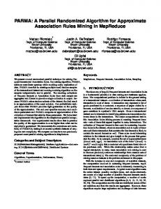
Note that RX (f ) can also be thought of the image of the continuous surjection map Φf : X → X∼ where Φf (x) = Φf (y) if and only if x and y come from the same connected component of a level set of f . In this sense, RX (f ) is obtained by continuously identifying each connected component C. The map Φf induces a scalar function f˜ : RX (f ) → IR on RX (f ) where f˜(p) = f (x) if p = Φf (x). Since f (x) = f (y) whenever Φf (x) = Φf (y), the function f˜ is well-defined. Since f is continuous, so is f˜. Reeb graph nodes and arcs. As the name suggests, the Reeb graph RX (f ) can be represented as a graph. See Figure 1 (b) for an example, where the height of a point q ∈ RX (f ) is simply f˜(q). Now for every point q ∈ RX (f ), there is a sufficiently small neighborhood R0 ⊆ RX (f ) containing q such that R0 is connected, has no loops, and f˜(p) 6= f˜(q) for any point p ∈ R0 − {q}. Let γ be a connected component of R0 − {q}. Since f˜(p) 6= f˜(q) for any point p ∈ γ and f˜ is continuous, either f˜(p) > f˜(q) for all p ∈ γ or f˜(p) < f˜(q) for all p ∈ γ. The up degree of a point q ∈ RX (f ) is the number of connected components γ in R0 − {q} where f˜(p) > f˜(q) for p ∈ γ. The down degree of q ∈ RX (f ) is the number of connected components γ in R0 − {q} where f˜(p) < f˜(q) for p ∈ γ. A node of RX (f ) is a point q ∈ RX (f ) whose up degree is not one or whose down degree is not one. Deleting the nodes of RX (f ) from RX (f ) leaves a set of curves which are the arcs of the Reeb graph. The Reeb graph RX (f ) encodes partial information about the 0-th and 1-st homology group information of the topological space X. Specifically, it can be shown [11] that β0 (R(f )) = β0 (X) and β1 (R(f )) ≤ β1 (X). If X is an orientable 2-manifold, then one can in fact obtain the full 1-st homology group information (including its rank and generators) about X from R(f ) [7]. Piecewise-linear (PL) settings. We consider a simplicial complex K and a piecewise-linear (PL) function f : K → IR defined on K. Specifically, f is defined at vertices of K, and linearly interpolated in the interior of every simplex of dimension higher than 0. Since R(f ) depends only on the connectivity of each level set, for a generic function f (where no two vertices have the same function value), the Reeb graph of f depends only on the 2-skeleton of K. Hence from now on, we assume that f is generic and K = (V, E, T ) is a simplicial 2-complex with vertices V , edges E and triangles T . r
Φf (r)
Φf (r) w
Φf (w)
Φf (w)
Φf (w)
q
Φf (q)
Φf (q) Φf (p)
p
Φf (p)
Φf (p)
(a)
(b)
(c)
(d)
Figure 1: A simplicial complex K in (a) and the Reeb graph of the height function is in (b). Shaded triangles are 2-simplices in K, and the two front faces of the tetrahedron pqrw as well as one back face 4qrw are present in K. The corresponding augmented Reeb graph is shown in (c). If the back face 4qrw is missing, then the corresponding augmented Reeb graph is shown in (d). One can obtain (b) by removing monotonic degree-2 nodes from (c). Augmented Reeb graph. An augmented Reeb graph of f : X → IR is a Reeb graph of f with some additional degree-2 vertices inserted in the original Reeb graph arcs. In particular, if f is a piecewiselinear function on a simplicial complex K, then the augmented Reeb graph generated by K is a Reeb graph of f whose nodes are {Φf (v) : v ∈ V (K)}. Note that all nodes of the original Reeb graph are in {Φf (v) : v ∈ V (K)}. See Figure 1 (c) and (d) for examples. One can obtain the original Reeb graph from
3
the augmented one by removing monotonic degree-2 nodes, which are nodes with up-degree 1 and downdegree 1. (The augmented Reeb graph generated by K is similar to the augmented contour tree in [5].) Some notations. Let f be a function on triangle t = 4pqr such that f (p), f (q) and f (r) are all distinct. The middle vertex of t, denoted by mid(t), is the vertex q where f (p) < f (q) < f (r). The edge of t opposite to mid(t), pr in this example, spans the range of function values for all points in t, and is called the spanning edge of t. Our initial input K is a simplicial complex. However, as our algorithm proceeds, we will obtain intermediate complexes that may no longer be simplicial. Specifically, there may be multiple edges between the same pair of vertices. Similarly, two triangles may have the same set of vertices but not the same set of edges. Hence we usually denote a triangle t by its boundary edges t(e1 , e2 , e3 ). However, for simplicity, we sometimes still denote a triangle by its vertices 4pqr when its choice of edges is clear.
4
Algorithm R AND R EEB
Input to Algorithm R AND R EEB is a simplicial 2-complex K = (V, E, T ) and a piecewise linear function f : K → IR. We assume that f (v) are distinct for all v ∈ V (K). We can enforce this condition by symbolically perturbing the scalar value at all vertices. The algorithm compute the augmented Reeb graph of f in expected time O(m log n) where n = |V | and m = |V | + |E| + |T | is the size of K. In what follows, after briefly describing the data structure our algorithm uses, we introduce main components of our algorithm. From now on, in all figures, we use the height function as the input piecewise-linear function f . Data structure. The set of vertices is stored in an array. The set of edges and triangles are each stored in a doubly-linked list. Each edge e maintains a list of (pointers to) triangles incident on e, denoted by IncT (e). Each triangle maintains three pointers to its three boundary edges, e1 , e2 and e3 , and three pointers to its position in these incident lists, IncT (e1 ), IncT (e2 ) and IncT (e3 ). Similarly, a vertex v maintains a list of triangles having v as middle-vertex, and each triangle stores a pointer to its position in the corresponding list. Adding or removing a triangle takes O(1) time. The total size of the data structure is O(|V |+|E|+|T |).
4.1
The Collapse Operation
e2 q
e1
r2
e2
e3 x
y
r1
p2
p2
(a)
e1
q
r
p2
p1
(b)
p2 e2
e3 e1
p1
r
e5
e2 q
q p1
p2
r
p2
e4
q
q0
p1
e6
q (=q 0 ) p1
e5
e1
r e4
p1
(c)
Figure 2: (a) Collapse(t) with t = (e1 , e2 , e3 ). All points from t on the same contour (e.g, segment xy) collapse onto its corresponding point on edges e1 or e2 (e.g, point y). (b) Edge e3 has three incident triangles other than t. (c) Each incident triangle of e3 , say 4rp1 p2 , will be split into two (4rp1 q 0 , 4rp2 q 0 with f (q) = f (q 0 )).
A fundamental operation of our algorithm is the Collapse(t) procedure defined for a triangle t. Let e1 and e2 be the edges of t incident on q = mid(t), and let e3 be the edge of t opposite q. Since e3 is the spanning edge of t, no two points in e1 ∪ e2 share the same function value. Procedure Collapse(t) collapses t by mapping {x ∈ t : f (x) = f (y)} to the point y ∈ e1 ∪ e2 . See Figure 2 (a) for an illustration.
4
Procedure C OLLAPSE(t) (1) remove triangle t (2) let q = mid(t), and e3 = (p1 , p2 ) the spanning edge of t (3) let e1 = (q, p1 ) and e2 = (q, p2 ) be the edges of t incident on q (4) merge all edges identified with e3 (5) For (every σ incident to e3 and σ 6= t) (6) set r be the vertex of σ opposite to e3 (7) let e4 = (r, p1 ) and e5 = (r, p2 ) be the edges of σ incident on r (8) If (r == q) // then t and σ have the same vertices (9) If (e1 6= e4 ) Then identifyEdges(e1 , e4 ); (10) If (e2 6= e5 ) Then identifyEdges(e2 , e5 ); (11) Else (12) create new edge e6 with endpoints q, r (13) create triangle (e1 , e4 , e6 ) and triangle (e2 , e5 , e6 ) (14) Endif (15) remove triangle σ; (16) Endfor (17) remove edge e3 ; Figure 3: Pseudo-code for the collapse operation. Collapsing t splits all the other triangles incident on the spanning edge e3 . Let σ = (e3 , e4 , e5 ) be a triangle incident on e3 , where e4 shares a vertex with edge e1 ∈ t and e5 shares a vertex with edge e2 ∈ t. Triangle σ has a vertex r opposite e3 . We add the edge e6 with endpoints q, r and replace σ with triangles (e1 , e4 , e6 ) and (e2 , e5 , e6 ). See Figure 2 (c). We refer to σ as a splitting triangle. Every incident triangle to edge e3 other than t itself is a splitting triangle. We remark that one should consider simplicial complexes in this paper as abstract simplicial complexes. After the collapse operation, it is possible that the geometric realization of the new complex in the embedding Euclidean space may have self-intersections. p2 Procedure Collapse described above may create double or even p2 r r multiple edges between the same two points. For example, see the figure on the right where the complex contains four faces of a tetra- q q hedron. Collapsing 4qp1 p2 splits 4p1 p2 r and creates a double p1 p1 edge between q and r. (Also, recall Figure 1 (b) where such a pair of double edge creates a loop in the final Reeb graph.) Hence the resulting complex may not be a simplicial complex any more, but rather, is a cell complex with the property that each face is a simplex. u u Because the complexes created by Procedure Collapse are not necessarily simplicial, a triangle σ incident to the spanning edge e3 of t may w w p2 p2 e5 have the same vertices as the collapsing triangle t (i.e, r = q in Figure e (= e ) 2 5 e2 e 2 (c)). In this case, edges e1 and e4 may be the same edges or they may q q 3 e1 be “double” edges, sharing the same endpoints but nevertheless distinct. p1 p1 Similarly, edges e2 and e5 may be the same edges or they may be distinct double edges. For example, in the figure on the right, there are two edges e2 and e5 between q and p2 and two triangles with the same set of vertices q, p1 , p2 . One triangle has edges e1 , e3 and e2 while the other one has edges e1 , e3 and e5 . In the case where σ and t share the same vertices, collapsing t and splitting σ would create two degenerate triangles, spanned by edges e1 and e4 , and by edge e2 and e5 , respectively. Instead of creating such
5
degenerate triangles, if edges e1 and e4 are distinct double edges, then we simply identify these two edges. Similarly, if edges e2 and e5 are distinct, then we identify e2 and e5 . In each case the algorithm calls a procedure to merge the two edges and their data structures into a single edge. In the previous example on the right, triangle t1 (e2 , qu, up2 ) is incident to edge e2 while triangle t2 (e5 , qw, wp2 ) is incident to edge e5 . Collapsing triangle t(e1 , e2 , e3 ) causes the deletion of triangle σ(e1 , e5 , e3 ) and the identification of edge e5 with e2 . After the identification of e2 and e5 , both t1 and t2 are incident to edge e2 and edge e5 is removed. The pseudo-code of Procedure Collapse is described in Figure 3. Finally, let K1 and K2 denote the complex before and after Procedure Collapse(t). Note that K1 and K2 share the same set of vertices V , and each cell in K2 is still a simplex. Let e1 and e2 be the edges of t incident on mid(t). Procedure Collapse(t) induces a continuous surjection φt : |K1 | → |K2 | where φt (y) = y if y ∈ / t, and φt (y) = φt (x) if y ∈ t and x ∈ e1 ∪ e2 and f (x) = f (y). Since each cell in K2 is still a simplex, it can be shown that the function ft : |K2 | → IR defined as ft := f ◦ φt is exactly the piecewise-linear function on K2 induced by the function values f (v) at v ∈ V . We thus abuse the notation slightly and still refer to ft as f . Lemma 4.1 Let K1 and K2 denote the complex before and after a collapse operation. The augmented Reeb graphs remains the same; that is, RK1 (f ) = RK2 (f ). Proof: Let Φ2 : |K2 | → RK2 (f ) be the surjection mapping K2 to its Reeb graph. Set Φ = Φ2 ◦φt . Function Φ maps each connected component of a level set to a distinct point. Thus RK2 (f ) equals RK1 (f ). Vertex-collapse with respect to q. A vertex-collapse w.r.t a vertex q, denoted by SeqCollapse(q), refers to a sequence of collapse operations for all triangles with q being the middle vertex. These triangles may include new triangles created from earlier collapse operations involving q. In fact, it is necessary that one of the two new triangles created by every splitting triangle during Collapse(t) will have q as the middle vertex, and thus will be later collapsed while executing SeqCollapse(q). For example, in Figure 2 (c), the triangle 4qp1 r may be later also collapsed in SeqCollapse(q). At the end of SeqCollapse(q) operation, there is no triangle left with q being the middle-vertex. In other words, SeqCollapse(q) provides a systematic way to collapse the entire contour passing through q onto q. See Figure 4 for an example.
q
q
(a)
(b)
Figure 4: (a) Before and (b) after vertex-collapse operation SeqCollapse(q). Shaded triangles are 2-simplices. Two dark-shaded triangles are not affected by this operation.
Claim 4.2 After performing SeqCollapse(q), no subsequent vertex-collapse operations can ever create a triangle with q being the middle vertex. Proof: Each splitting triangle σ will create two new triangles σ1 and σ2 . The key observation is that the two extreme vertices of σ (i.e, the vertex with largest and smallest function values) remain extreme in the new triangles. Hence after Procedure SeqCollapse(q) (at which point q is not the middle-vertex of any triangle), no subsequent collapse operation can change q from being an extreme vertex of some triangle to being the middle vertex of another triangle. The claim then follows. 6
4.2
Identifying Edges
The last remaining operations to describe are the identifyEdges(e, e0 ) in Steps (9) and (10) of Procedure Collapse and the merging of these edges in Step (4) in Figure 3. The simplest way to implement identifyEdges is to traverse the lists of triangles, IncT (e) and IncT (e0 ), merging the two lists into one and updating the incident triangles. However, this merging and updating associated data-structures of incident triangles takes time proportional to the length of one of the two lists. If the simplicial complex is a 2manifold, then each list IncT (e) never has more than two elements (see Appendix B). However, for a general simplicial complexe, these lists may grow arbitrarily long. To ensure that Steps (9) and (10) do not take too much time, we use a “lazy” identification procedure. Specifically, instead of merging e and e0 and their associated data structures, identifyEdges(e, e0 ) simply records the identity relation between e and e0 . Each edge has a list of edges with which it has a identityrelation. Calling identifyEdges(e, e0 ) adds e0 to the list of e and adds e0 to the list of e. The actual merging of edges only occurs in Step (4) of Procedure Collapse. All the edges identified transitively with the spanning edge e3 and their associated incident triangle lists are merged with e3 . Note e3 is removed at the end of the call to Collapse(t). All the edges identified with e3 and all the triangles incident on those edges are also removed in this call. Thus, each edge is only involved in one merge operation.
4.3
The Randomized Algorithm
Algorithm R AND R EEB(K, f ) randomly permutes vertices of K and performs SeqCollapse(v) for each vertex v in the permuted order. Because of lazy edge identification, some edges may be identified but not yet merged. As a final step, R AND R EEB merges these edges using a linear scan. Termination. Algorithm R AND R EEB calls Procedure SeqCollapse(v) for each vertex v of K. Procedure SeqCollapse(v) calls Collapse(t) for each triangle t whose middle vertex is v. Procedure Collapse(t) can create new triangles whose middle vertex is t. However, the number of such triangles is bounded by the number of triangles intersected by the level set f − (v). Therefore, SeqCollapse(v) creates only a finite number of new triangles and Algorithm R AND R EEB terminates. Correctness. Let (v1 , v2 , . . . , vn ) be the vertices of K listed in the order their permuted order. At the i’th iteration of the algorithm, any triangle with middle vertex vi will be collapsed. By Claim 4.2, no new triangle can be created with middle vertex vi after the i’th iteration. Hence no triangle with middle vertex vi can remain at the end of the algorithm, for any i ∈ [1, n]. Thus, Algorithm R AND R EEB constructs a graph G = (V, Er ), possibly with multiple edges having the same endpoints. Finally, note that the algorithm is simply a sequence of Collapse procedures. By Lemma 4.1, Procedure Collapse does not change the Reeb graph. Thus, the final outcome, which is itself a graph, is exactly the augmented Reeb graph RK (f ).
4.4
Time Complexity
We now analyze the time complexity of the above randomized algorithm R AND R EEB(K, f ). The worst case time complexity is Ω(|V ||T |) even when K is a 2-manifold without boundary. A lower-bound example is shown in Appendix A. We now claim that for an arbitrary simplicial 2-complex K, the expected running time of R AND R EEB is O(m log n). Below we first argue that each Collapse procedure takes time proportional to the number of triangles it collapses and splits. We then bound the (expected) total number of triangles that will ever be collapsed or split.
7
One collapse operation. Given a triangle t = (e1 , e2 , e3 ) with spanning edge e3 , Collapse(t) destroys all k = |IncT (e3 )| triangles incident to edge e3 , and creates at most 2(k − 1) new triangles. Destroying the triangle t itself takes O(1) time. Consider a splitting triangle σ incident to e3 . If σ and t do not share the same vertices, then splitting σ creates two new triangles, which can be done in O(1) time. If they share the same vertices, then edges e1 and e4 (or e2 and e5 ) may need to be identified. Using lazy edge identification, the identity relation between e1 and e4 is recorded in O(1) time. Thus Steps (5)–(17) run in time O(k). Step (4) merges all the edges identified with e3 , as well as their lists of incident triangles. Since each incident triangle merged becomes an entry in IncT (e3 ), merging all incident triangles takes O(|IncT (e3 )|) = O(k) time. The cost of finding and merging all edges identified with e3 in a transitive way is proportional to the total number of identify-relations recorded in all these edges. We charge the cost of processing each entry to the cost of creating this identity relation in Steps (9) and (10). Since each identity relation, once processed, will be destroyed, each Step (9) or (10) is charged at most once. Thus bounding the total time of Steps (5)–(17) over all calls to Procedure Collapse bounds also the total time for Step (4). Overall analysis. The above analysis says that the total time for all executions of Step (4) is bounded by the total time for all executions of Steps (5)–(17). Hence the total number of triangles ever destroyed provides an upper bound for Algorithm R AND R EEB. We now focus on bounding total number of triangles ever destroyed. Note that a triangle σ can be destroyed either by performing Collapse procedure on this triangle itself, or by splitting it while collapsing some other triangle. We call σ a collapsing triangle in the former case, and a splitting triangle as usual in the latter case. If σ is a collapsing triangle, then it will not create any new triangle. Now suppose σ is split while performing Procedure Collapse(t). If σ shares the same vertices with t, then we call it a degenerate splitting triangle. In this case, it will not create any further triangle either. Otherwise, it is a non-degenerate splitting triangle, and creates two new triangles σ1 and σ2 . Exactly one of the new triangles, say σ2 , has the same middle-vertex as q = mid(t) (e.g, σ2 = 4qp1 r in Figure 2 (c)). Hence σ2 will be destroyed within the same SeqCollapse(q) operation as Collapse(t), either being collapsed or split. In fact, if σ2 is destroyed by splitting, then σ2 is destroyed when the algorithm collapses another triangle t0 that shares the same vertices as σ2 . In this case σ2 is a degenerate splitting triangle. In summary, whether σ2 is a collapsing or a splitting triangle, it will be destroyed within Procedure SeqCollapse(q), and will not create any new triangle. The other new triangle σ1 will remain untouched throughout the SeqCollapse(q) operation. NS We now charge the existence of the short-lived triangle σ2 to σ. On the other hand, we say that σ1 is the child of the splitting triangle σ, and σ is the parent of σ1 . If σ1 turns out to DS/C NS be also a collapsing triangle, we charge it to σ as well. In summary, each splitting triangle has at most one child, and can be charged at most twice. These relations are illustrated in the right DS/C figure, where ’NS’, ’DS’ and ’C’ stand for non-degenerate splitting, degenerate splitting, and NS collapsing triangles, respectively. Solid segments indicate parent-child relations, and dotted segments indicate charging relations. Note that the parent-child relations induce a collection DS/C of directed paths (the solid path in the right figure is one example). Each such path starts with DS/C a triangle t ∈ T from the original complex K, consists of a sequence of non-degenerate splitting triangles descended from t, and ends with either a collapsing triangle or a degenerate splitting triangle. We call such a path the descendant-path with head t. There are exactly |T | number of descendant-paths, each headed by an original triangle from K. If an original triangle is a collapsing triangle, then its descendant-path has length 1 (containing only itself). Every non-degenerate splitting triangle belongs to exactly one descendant-path. The total size of these paths upper-bounds the total number of splitting and collapsing triangles ever existed. We now bound the expected length of each descendant-path.
8
Expected length of a descendant-path. Let the index of a vertex v ∈ V , denoted by I(v), be its position in the sorted list of vertices based on their function values; that is, f (vi ) > f (vj ) if and only if I(vi ) > I(vj ). Given a triangle t = 4abc, the range of t, denoted by rg(t), is the interval spanned by maximum and minimum indices of vertices of t; that is, rg(t) = [min{I(a), I(b), I(c)}, max{I(a), I(b), I(c)}]. Now consider a non-degenerate splitting triangle σ with range rg(σ) = [I1 , I2 ]. Let Vσ ⊆ V be the set of vertices v of K such that (1) f (v) ∈ rg(σ), and (2) σ intersects the level set connected component containing v. Obviously, as we perform SeqCollapse(v) for some v ∈ Vσ , triangle σ will either be collapsed (thus terminating the descending-path it lies in), or be split. In the latter case, the range of its child σ1 is either [I1 , I(v)] or [I(v), I2 ]. In either case, R(σ1 ) is strictly contained in the range rg(σ) of σ. Furthermore, if we choose v randomly from Vσ , then with constant probability, the size of Vσ1 is at most half of that of Vσ . Thus intuitively, it can be further split O(log |Vσ |) = O(log |V |) expected number of times. This can be made more precise by a standard probabilistic analysis using indicator functions for the length of the range that may appear in a dependent-path with a fixed head. Alternatively, this can be seen by thinking of this splitting process as building a randomized binary search tree, where splitting σ against a vertex q ∈ Vσ corresponds to insert a random key I(q). At each node of the tree, we record the range of keys in its subtree. The sequence of ranges of triangles on the descendant-path with head σ corresponds to ranges of nodes along some tree path in a randomly built binary tree over keys I1 , I1 + 1, . . . , I2 . Since the expected height of such a tree is O(log(I2 − I1 )) = O(log |V |) [8], the dependent path has expected length of O(log |V |). Since there are |T | number of descendant-paths, putting everything together, we conclude with our main result: Theorem 4.3 Given an arbitrary simplicial complex K with 2-skeleton (V, E, T ) and a piecewise-linear function f : K → IR, Algorithm R AND R EEB(K, f ) computes the augmented Reeb graph R(f ) in expected time O(m log n) where m = |V | + |T | + |E| and n = |V |.
4.5
Variations
2-manifolds. When K is the triangulation of a 2-manifold, there is no need to use lazy edge identification. Thus Algorithm R AND R EEB can be simplified while retaining its O(|V | log |V |) expected running time. The details can be found in Appendix B. Using potential critical points. As we sweep K in increasing function values, the 0-th homology of the level sets does not change till some “critical” moments (corresponding to nodes in the Reeb graph). For example, if |K| is a manifold and f is a Morse function, then these critical moments correspond to a certain subset of critical points of f . Instead of applying the SeqCollapse(v) to all the vertices of K, we need only apply it to the “critical” vertices of K. We identify a subset of vertices Vc ⊆ V which we call potential critical points, randomly permute them, and then apply Procedure SeqCollapse to these vertices in their permuted order. The resulting complex is not a graph, but it turns out that the Reeb graph can be easily extracted from this complex in linear time. The time complexity of running R AND R EEB using only the critical vertices is O(m log |Vc |) = O(m log n). In the worst case, this running time is the same as the running time when all vertices are processed, but the revised algorithm is faster when |Vc | is substantially smaller than m. The details are in Appendix C.
5
Experiments
We implemented Algorithm R AND R EEB() using the version where we only collapse w.r.t potential critical points as discussed in Section 4.5. In our experiments, this usually improves the running time of the version that processes all points by 10%–50%. Experiments are conducted on a standard desktop with a 64-bit 3.16 GHz Intel Core 2 Duo CPU and 8 GB of RAM. Most data are courtesy of the AIM@SHAPE database [1]. 9
Performance comparison. We compare the performance of our algorithm with that of two state-of-the-art algorithms: the output-sensitive algorithm proposed in [9], denoted by OS, and the loop-surgery algorithm proposed in [26], denoted by LS. Algorithm OS can handle arbitrary simplicial complexes. We use the original implementation of OS kindly provided by the authors of [9]. Algorithm LS processes only tetrahedral meshes modeling 3-manifolds with boundary embedded in IR3 . We use published running times reported in [26], which were obtained on a computer of similar configuration as ours. Time for our algorithm is averaged over 5 runs. Table 5 compares the running times of the three algorithms on a set of tetrahedral meshes of volumetric data (i.e, 3-manifolds with boundary embedded in IR3 ) used in previous papers [9, 26], and on a set of non-manifold simplicial complexes. See Appendix D.1 for a description of the non-manifold data.
Classification
Tetrahedron
Non-manifold
Dataset Statistics Dataset #Triangles Fighter 143881 Plasma 2646016 Earthquake 4198057 Buckyball 2524284 Post 1243200 Hand 1676884 Camel 144971 104127 Simulation
|Vc | 3618 2852 11896 4378 132 209 176 11804
# Loops 0 0 0 0 1 0 24 214
Running Time (sec) Our OS [9] LS [26] 5.36 629.40 0.35 114.76 3772.42 2.20 150.28 5866.71 4.07 56.75 1602.01 2.51 13.91 18.05 0.69 6.60 14.10 * 0.26 0.86 * 1.31 193.966 *
Table 2: Entries marked with * are unavailable. Vc is the set of potential critical points used by our algorithm. Our algorithm outperforms algorithm OS in all cases. Algorithm LS is specifically designed for 3manifolds with boundary embedded in IR3 and gives superior performance on all tetrahedral meshes. Both our algorithm and algorithm LS identify and use a few potential critical points. Based on a nice observation about 3-manifolds embedded in IR3 , Algorithm LS processes only critical points which form a loop in the Reeb graph of the boundary of the 3-manifold. Thus its running time depends on the number of loops in this Reeb graph. While [26] reported timing results for some tetrahedral meshes whose boundary Reeb graphs contained 30-80 such loops, these data sets are not in the public domain. The tetrahedral mesh data sets listed in Table 5 all have 0 or 1 loops. Since the observation used in [26] does not hold for arbitrary simplicial complexes, Algorithm R AND R EEB needs to consider a much larger set of potentially critical points, not just the ones contributing to loops in the Reeb graph of domain boundary. The number of such points are on the order of several thousands in the data sets we tested. (See column 4 in Table 5). Effect of random collapsing. To measure the effect of collapsing in random order, we removed randomization from R AND R EEB and called SeqCollapse on potential critical points in order of increasing function values. We counted the average number of times an input triangle was split by the original randomized version of R AND R EEB (AvgRand) and by the sequential, non-random version (AvgSeq). The Fighter data has 3618 potential critical points, R AND R EEB splits each triangle 21.16 times on average, while the sequential version splits each triangle 1138 times on average. Note that 21 is on the order of log2 (1138) which is what we expect by using a random order of collapsing. (Appendix D.2 contains statistics for other data.) Let Cq denote the connected component of f −1 (q) that contains vertex q. AvgSeq is a lower bound on the number of times that a triangle intersects Cq for all potential critical points q. Thus each triangle in the Fighter data set intersects an average of (at least) 1138 such connected components. This may in some sense explain the performance difference between our algorithm and algorithm OS from [9], as algorithm OS may process a triangle every time it is intersected by such a connected component.
10
References [1] Aim@shape shape repository, 2006. http://shapes.aimatshape.net/. [2] M. Attene, S. Biasotti, and M. Spagnuolo. Shape understanding by contour driven retiling. The Visual Computer, 19(2-3):127–138, 2003. [3] S. Biasotti, B. Falcidieno, and M. Spagnuolo. Extended Reeb graphs for surface understanding and description. In Proc. 9th Internat. Conf. Discrete Geom. for Computer Imagery, pages 185–197, 2000. [4] S. Biasotti, D. Giorgi, M. Spagnuolo, and B. Falcidieno. Reeb graphs for shape analysis and applications. Theor. Comput. Sci., 392(1-3):5–22, 2008. [5] H. Carr. Topological manipulation of isosurfaces. PhD thesis, The University of British Columbia (Canada), 2004. Adviser-Panne, Michiel Van. [6] H. Carr, J. Snoeyink, and U. Axen. Computing contour trees in all dimensions. Comput. Geom, 24(2):75–94, 2003. [7] K. Cole-McLaughlin, H. Edelsbrunner, J. Harer, V. Natarajan, and V. Pascucci. Loops in Reeb graphs of 2-manifolds. Discrete Comput. Geom., 32(2):231–244, 2004. [8] T. H. Cormen, C. E. Leiserson, R. L. Rivest, and C. Stein. Introduction to Algorithms. MIT Press, Cambridge, MA, second edition, 2001. [9] H. Doraiswamy and V. Natarajan. Efficient output-sensitive construction of Reeb graphs. In Proc. 19th Internat. Sym. Alg. and Comput., pages 556–567, 2008. [10] H. Doraiswamy and V. Natarajan. Efficient algorithms for computing Reeb graphs. Computational Geometry: Theory and Applications, 42:606–616, 2009. [11] H. Edelsbrunner and J. Harer. Computational Topology. An Introduction. Amer. Math. Soc., Providence, Rhode Island, 2009. [12] H. Edelsbrunner, J. Harer, A. Mascarenhas, V. Pascucci, and J. Snoeyink. Time-varying Reeb graphs for continuous space-time data. Comput. Geom., 41(3):149–166, 2008. [13] F. H´etroy and D. Attali. Topological quadrangulations of closed triangulated surfaces using the Reeb graph. Graph. Models, 65(1-3):131–148, 2003. [14] M. Hilaga, Y. Shinagawa, T. Kohmura, and T. L. Kunii. Topology matching for fully automatic similarity estimation of 3d shapes. In Proc. SIGGRAPH ’01, pages 203–212, 2001. [15] P. Kanongchaiyos and Y. Shinagawa. Articulated Reeb graphs for interactive skeleton animation. In S. Hashimoto, editor, Multimedia Modeling: Modeling Multimedia Information and System, pages 451–467. World Scientific, 2000. [16] I.-H. Park and C. Li. Novel dynamic ligand-induced-fit simulation via enhanced conformational samplings and ensemble dockings: a survivin example, 2009. Submitted to The Journal of Physical Chemistry, B. [17] V. Pascucci, G. Scorzelli, P.-T. Bremer, and A. Mascarenhas. Robust on-line computation of Reeb graphs: simplicity and speed. ACM Trans. Graph., 26(3):58, 2007.
11
[18] G. Patan`e, M. Spagnuolo, and B. Falcidieno. Para-graph: Graph-based parameterization of triangle meshes with arbitrary genus. Comput. Graph. Forum, 23(4):783–797, 2004. [19] G. Reeb. Sur les points singuliers d’une forme de Pfaff compl`etement int´egrable ou d’une fonction num´erique. Comptes Rendus Hebdomadaires des S´eances de l’Acad´emie des Sciences, 222:847–849, 1946. [20] Y. Shi, R. Lai, S. Krishna, N. Sicotte, I. Dinov, and A. W. Toga. Anisotropic Laplace-Beltrami eigenmaps: Bridging Reeb graphs and skeletons. Computer Vision and Pattern Recognition Workshop, 0:1–7, 2008. [21] Y. Shinagawa and T. L. Kunii. Constructing a Reeb graph automatically from cross sections. IEEE Comput. Graph. Appl., 11(6):44–51, 1991. [22] Y. Shinagawa, T. L. Kunii, and Y. L. Kergosien. Surface coding based on morse theory. IEEE Comput. Graph. Appl., 11(5):66–78, 1991. [23] J. Sun, M. Ovsjanikov, and L. J. Guibas. A concise and provably informative multi-scale signature based on heat diffusion. Comput. Graph. Forum, 28(5):1383–1392, 2009. [24] S. P. Tarasov and M. N. Vyalyi. Construction of contour trees in 3D in o(nlogn) steps. In Proc. 14th Annu. ACM Sympos. Comput. Geom., pages 68–75, 1998. [25] J. Tierny. Reeb graph based 3D shape modeling and applications. PhD thesis, Universite des Sciences et Technologies de Lille, 2008. [26] J. Tierny, A. Gyulassy, E. Simon, and V. Pascucci. Loop surgery for volumetric meshes: Reeb graphs reduced to contour trees. IEEE Trans. Vis. Comput. Graph., 15(6):1177–1184, 2009. [27] T. Tung and F. Schmitt. The augmented multiresolution Reeb graph approach for content-based retrieval of 3d shapes. Internat. J. Shape Modeling, 11(1):91–120, 2005. [28] M. van Kreveld, R. van Oostrum, C. Bajaj, V. Pascucci, and D. Schikore. Contour trees and small seed sets for isosurface traversal. In Proc. 13th Annu. ACM Sympos. Comput. Geom., pages 212–220, 1997. [29] Z. Wood, H. Hoppe, M. Desbrun, and P. Schr¨oder. Removing excess topology from isosurfaces. ACM Trans. Graph., 23(2):190–208, 2004. [30] E. Zhang, K. Mischaikow, and G. Turk. Feature-based surface parameterization and texture mapping. ACM Trans. Graph., 24(1):1–27, 2005.
12
A
Lower-bound Example for Algorithm R AND R EEB rn−2
rn−2
r r The worst case time complexity for our algorithm r r r r R AND R EEB(K, f ) is Ω(|V ||T |) even when K is a p p r r 2-manifold without boundary. A lower-bound example for a manifold with boundary is shown in the p p right figure. In this example, we process the vertices p p {p1 , p2 , . . . , pn } in order. Each SeqCollapse(pi ) p p q q will destroy all Θ(n) triangles of the form 4pi−1 rj rj+1 and create Θ(n) triangles of the form 4pi rj rj+1 . Simple modifications of the figure on the right give a worst case Ω(|V ||T |) bound for a 2-manifold without boundary. 1
1
n−1
n−1
2
2
n
n
1
3
3
2
2
1
B
1
1
2-Manifolds
When K is the triangulation of a 2-manifold, it turns out that there is no need to use lazy edge identification. Thus Algorithm R AND R EEB can be simplified while retaining its O(|V | log |V |) expected running time. The simplification is based on the following. With this property, there is no longer any need to use lazy edge identification, since performing merging directly in Steps (9) and (10) takes constant time. Claim B.1 If K is the triangulation of a 2-manifold (with or without boundary,) then |IncT (e)| ≤ 2 for any edge e in any intermediate complex produced by R AND R EEB(K, f ). Proof: The claim holds at the beginning for K, since its underlying space is a 2-manifold. Let IncTK 0 (e) denote the incident list of an edge e in an intermediate complex K 0 . Let K1 and K2 be the complex before and after a Collapse(t) operation with t = 4(qp1 p2 ) and q = mid(t). Recall Figure 2. After the collapse operation, edge qp1 will lose one incident triangle (which is t), but gain k − 1 incident triangles where k = |IncTK1 (p1 p2 )| Hence |IncTK2 (qp1 )| = |IncTK1 (qp1 )| − 1 + (k − 1) ≤ 2 as both |IncTK1 (qp1 )| and k are bounded by 2. The same argument holds for edge qp2 . For each splitting triangle σ = 4p1 p2 r involved in Collapse(t), if r 6= q, then the boundary edges p1 r and p2 r will lose one triangle (i.e, σ) but gain one triangle 4qp1 r (resp. 4qp2 r). Hence the size of its incident list remains the same. In the case that r = q and a pair of double edges e1 and e2 are identified, we have that |IncTK2 (e1 )| = |IncTK1 (e1 )| − 1 + |IncTK1 (e2 )| − 1 ≤ 2. The claim thus holds at any time during the algorithm.
C
Using Potential Critical Points
Algorithm R AND R EEB is conceptually simple and easy to implement. However, it ignores any property that input data may have. Specifically, observe that as we sweep K in increasing function values, the H0 homology of the level sets does not change till some “critical” moments (corresponding to nodes in the Reeb graph). For example, if the |K| is a 2-manifold (resp. d-manifold) and f is a Morse function, then these critical moments correspond to the set of critical points (resp. a certain subset of critical points) of f . Thus it seems wasteful that we perform Procedure SeqCollapse for all vertices in K, even though many of them do not carry key information.
13
We thus present a revised algorithm R AND R EEB(K, f ) to potentially reduce the number of Collapse operations. First, we say that a simplex α1 is lower (resp. higher) than another simplex α2 , if for any two points x and y in the interior of α1 and α2 , respectively, we have f (x) < f (y) (resp. f (x) > f (y)). Given a vertex v ∈ K, its lower star (resp. upper star) is the union of the interior of simplices incident to v which are lower (resp. higher) than v. See the right figure for an example: The left illustration shows the closure of all simplices incident to the empty dot, and the right one shows its lower star, which contains three components. We say that a vertex v ∈ K is a potential critical point if its lower star or upper star has more than one component. It is easy to verify that the pre-image of any node in the Reeb graph RK (f ) necessarily contains a potential critical point. The inverse is not true – the image of a potential critical point v may be a monotonic degree-2 point in the interior of an arc of RK (f ). We now modify Algorithm R AND R EEB() as follows. First, it computes the set of potential critical vertices Vc ⊆ V . In the second step, we randomly permute vertices in Vc and perform Procedure SeqCollapse for only these vertices. Let K 0 denote the resulting complex after these SeqCollapse operations. By Lemma 4.1, K 0 shares the same Reeb graph as K; that is, RK 0 (f ) = RK (f ). Furthermore, the following result suggests that K 0 almost has the structure of its Reeb graph, even though it is not a graph. Lemma C.1 Let Φf : |K 0 | → RK 0 (f ) be the continuous surjection from K 0 to its Reeb graph. For every point v ∈ V , there is a one-to-one correspondence between components in the upper-star of v in K 0 and the up-branches of Φf (v) in R(f ). Similarly, there is a one-to-one correspondence between components in the lower-star of v in K 0 and the lower-branches of Φf (v) in R(f ). See the right figure for an example where the underlying domain of input simplicial complex is a torus. There are four potential critical points in Vc in this case (empty dots). Consider the lower saddle point. Note that its lower star in the input manifold has two components. After performing SeqCollapse for all points in Vc in K 0 (middle figure), its lower star has only one component, just like in the final Reeb graph (right figure). Lemma C.1 states that the local neighborhood of every vertex in K 0 has the same connected component information as its image in the Reeb graph R(f ). Hence in the third step of the algorithm, we use K 0 to connect vertices in Vc to obtain the Reeb graph of f 1 . In particular, for every v ∈ Vc and for each component of its upper star, we start an upward path by connecting v to an arbitrary vertex v 0 of K in the closure of that component. We then connect v 0 to an arbitrary vertex v 00 connected to v 0 by an edge and with a higher function value. We continue this tracing until we reach another potential critical vertex from Vc . Note that any intermediate vertex we reach along this upward path can have only one component in its upper star (as otherwise, this vertex should be in Vc and the tracing is terminated). It follows from Lemma C.1 that the resulting graph consisting of the upward tracing paths is the Reeb graph of f . It is easy to see that the expected time complexity of the revised algorithm R AND R EEBis O(m log |Vc |) = O(m log n). In worst case this is the same as as the running time when processing all vertices, but is faster when Vc is substantially smaller than n. 1
Note that this is not the augmented Reeb graph generated by K any more, as not all vertices will appear as a node in the final Reeb graph. It is a Reeb graph of f augmented by some vertices from K.
14
D D.1
More on Experiments Data Sets
The tetrahedral meshes are downloaded from AIM@SHAPE database [1], and were used in previous papers [9, 26]. For non-manifold data set, the Simulation data is obtained by constructing the Rips complex from a set of high-dimensional points, where each point corresponds to a protein conformation produced by a molecular simulation process [16]. The function value at a point is the energy of the corresponding protein conformation. The Camel data is the Rips complex constructed from an incomplete point clouds of a camel model. The function value is the heat-signature defined in [23]. The Hand data is obtained from AIM@SHAPE database.
D.2
Effect on Random Collapse Dataset Fighter Plasma Earthquake Buckyball Blunt Post Hand Camel Simulation
# Triangles 143881 2646016 4198057 2524284 451601 1243200 1676884 144971 104127
|Vc | 3618 2852 11896 4378 827 132 209 176 11804
AvgSeq 1138.40 * * 104.3 103.6 9.97 2.34 3.44 40.92
AvgRand 21.16 15.57 13.95 11.1 12.46 5.62 2.3 3.16 7.64
Table 3: The average number of times an input triangle is split, using sequential vertex-collapsing (AvgSeq) and random vertex-collapsing (AvgRand). Only input triangles that are destroyed are counted when computing this average. Vc is the set of potential critical points that our algorithm processes. Entries marked with (*) as the algorithm runs out of memory when using sequential vertex-collapsing operations.
15