Hedman et al. BMC Research Notes 2010, 3:290 http://www.biomedcentral.com/1756-0500/3/290
RESEARCH ARTICLE
Open Access
A ranking index for quality assessment of forensic DNA profiles forensic DNA profiles Johannes Hedman1,2, Ricky Ansell1,3, Anders Nordgaard1,4*
Abstract Background: Assessment of DNA profile quality is vital in forensic DNA analysis, both in order to determine the evidentiary value of DNA results and to compare the performance of different DNA analysis protocols. Generally the quality assessment is performed through manual examination of the DNA profiles based on empirical knowledge, or by comparing the intensities (allelic peak heights) of the capillary electrophoresis electropherograms. Results: We recently developed a ranking index for unbiased and quantitative quality assessment of forensic DNA profiles, the forensic DNA profile index (FI) (Hedman et al. Improved forensic DNA analysis through the use of alternative DNA polymerases and statistical modeling of DNA profiles, Biotechniques 47 (2009) 951-958). FI uses electropherogram data to combine the intensities of the allelic peaks with the balances within and between loci, using Principal Components Analysis. Here we present the construction of FI. We explain the mathematical and statistical methodologies used and present details about the applied data reduction method. Thereby we show how to adapt the ranking index for any Short Tandem Repeat-based forensic DNA typing system through validation against a manual grading scale and calibration against a specific set of DNA profiles. Conclusions: The developed tool provides unbiased quality assessment of forensic DNA profiles. It can be applied for any DNA profiling system based on Short Tandem Repeat markers. Apart from crime related DNA analysis, FI can therefore be used as a quality tool in paternal or familial testing as well as in disaster victim identification.
Background The object of forensic DNA analysis is to generate individual-specific DNA profiles from crime scene stains and reference samples, thereby linking perpetrators to crimes. The analytical process includes sampling, DNA extraction/purification, and amplification of certain genetic markers (Short Tandem Repeats, STR) using the polymerase chain reaction (PCR). The actual DNA profile is generated by capillary electrophoresis separation of DNA fragments and detection using fluorescently labeled primers. An electropherogram (EPG) is produced where the intensity of the allelic peaks corresponds to the amount of produced DNA fragments, and the balance between peaks gives information on the reliability of the DNA profile (Figure 1). The amount and purity of the DNA is determined by all steps in the analytical process and subsequently affect the quality of * Correspondence:
[email protected] 1 Swedish National Laboratory of Forensic Science (SKL), SE-581 94 Linköping, Sweden Full list of author information is available at the end of the article
the EPG/DNA profile. Consequently, assessment of DNA profile quality is vital both for establishing the evidentiary value of a certain DNA profile and for comparing the relative performance of different DNA analysis protocols, e.g., in validation studies. In the last years, several statistical models and expert systems have been developed to streamline and simplify the routine evaluation of forensic DNA profiles [1-3], to aid in the interpretation of mixed DNA profiles [4,5] and to estimate the risk of encountering artifact peaks and/or allelic drop-outs [6-9]. However, assessment of DNA profile quality is generally not quantified or treated in an unbiased way. For example, in most studies comparing the performance of different forensic DNA analysis protocols, DNA profile quality is either assessed by manual examination based on empirical knowledge, and/or by comparing the intensities (allelic peak heights or areas) of the EPG/DNA profiles [10-14]. Manual examination has its apparent drawbacks in the difficulty for reproducibility and automation. The intensity is a
© 2010 Nordgaard et al; licensee BioMed Central Ltd. This is an Open Access article distributed under the terms of the Creative Commons Attribution License (http://creativecommons.org/licenses/by/2.0), which permits unrestricted use, distribution, and reproduction in any medium, provided the original work is properly cited.
Hedman et al. BMC Research Notes 2010, 3:290 http://www.biomedcentral.com/1756-0500/3/290
Page 2 of 10
Figure 1 Two EPGs/DNA profiles obtained from DNA analysis of a crime scene DNA sample using two different DNA polymerases. The DNA profiles were generated using A) standard AmpliTaq Gold DNA polymerase and B) an alternative DNA polymerase. The sample is a swab from a spoon found in a honey jar, with a DNA concentration of 0.09 ng/μl. Primers from the AmpFlSTR SGM Plus kit were used for both analyses. Peak heights are given in relative fluorescence units (rfu).
Hedman et al. BMC Research Notes 2010, 3:290 http://www.biomedcentral.com/1756-0500/3/290
decent quality measure but may be misleading if the allelic peak balance is not taken into account. We recently developed the forensic DNA profile index (FI), a ranking index for unbiased and quantitative quality assessment of forensic DNA profiles [15]. FI combines intensity and balance into one single, easily interpretable numerical index. FI is constructed by using Principal Components Analysis (PCA) on the following DNA profile quality measures: total allelic peak height (intensity), balance between allelic peaks within heterozygous loci (intra-locus or local balance), and balance between STR markers (inter-loci or global balance). The ranking index is based on empirical data taking into account statistical properties of such data as well as common opinions about what is considered a high or low quality EPG/DNA profile. Here we present the construction of FI, describing the applied mathematical and statistical methodologies. We show how to adapt the ranking index for any STR-based forensic DNA typing system through validation against a manual grading scale and calibration against a specific set of DNA profiles.
Methods and results This section describes the construction of the ranking index. First, we define the three quality measures that are used to create FI, and show how PCA is used to combine these measures into one single value. Second, we describe how FI is validated against a manual grading scale and how it may be calibrated against a calibration set of DNA profiles. Methodology Basic measures of DNA profile quality
Consider the EPG/DNA profile presented in Figure 1A. An experienced reporting officer would have no problems to identify what is acceptable or not in this DNA profile. However, there is no obvious way of immediately ranking the DNA profile without careful comparisons with other “competing” profiles. For that we need to define what we are supposed to look for in the EPG and how our observations could be summarized in a more compact way. This section generally follows what was published in Hedman et al. (2009), but with more details on central statistical issues. Central for all quality comparisons between DNA profiles is the study of allelic peak heights or peak areas, generally given in relative fluorescence units (rfu). Pronounced peak heights (i.e., peaks that extend clearly above the baseline) give information about which alleles are present and thus which loci are homozygous and which are heterozygous. Large peak heights generally indicate high quality while low heights are less desirable from a quality perspective. For a common measure of
Page 3 of 10
the allelic peak heights, the most straightforward alternative is the sum of all observed and approved peak heights in an EPG. More specifically we define the Total sum of Peak Heights, TPH, as TPH = ∑ M PH i , where i =1 M is the number of STR-loci analysed, and PHi is the sum of the two peak heights in locus i for a heterozygous locus, or the height the single peak of locus i for a homozygous locus. The measure is dominant for a DNA profile to be assessed as high quality, and the higher the value the higher the profile quality, provided fluorescence saturation is avoided by not overloading DNA template. Consider the two allelic peaks in the heterozygous D3S1358 locus in Figure 1A (top panel, left). For a DNA profile to be considered as high quality, discrepancies between the heights of the two allelic peaks in a heterozygous locus, such as this, should generally be small. With another wording we would strive for intralocus balance. For a heterozygous locus the ratio between the heights of the lower and the higher peak is a marker-specific measure of the balance between the peak heights. This measure lies between 0 and 1, where 1 is attained when the two peak heights are identical, and 0 represents a case where one of the peaks is not observed although it can be claimed to exist, a so-called drop-out allele. For a true homozygous marker, the measure is set to 1 to be consistent with the definition for heterozygous markers. In mathematical terms the balance measure for locus i may be written ⎧ Height of the lower peak ⎪ LBi = ⎨ Height of the higher peak ⎪1 ⎩
for a heterozygous locus for a (true) homozygous locus
A global measure of intra-locus or local balance is then obtained by taking the mean of these measures for all observed markers (Mean Local Balance): M MLB = M −1 ∑ i =1 LBi , where M is the number of ana-
lyzed STR markers. MLB is genotype dependent: DNA profiles from different people have different setups of homo- and heterozygous STR markers, affecting the measure. The extreme is that a person only has homozygous loci. In this case, all resulting DNA profiles would get a MLB equal to 1, as long as there are no drop-outs. Discrepancies between summarized peak heights between loci (Figure 1) are less straightforwardly handled. One approach could be to apply a measure of dispersion, like the standard deviation, but as such a measure is scale-dependent, data need to be standardized before it can be applied. We instead suggest to use the Shannon entropy [16], which in our case is defined as SH = −∑ p i ⋅ ln ( p i ) , where p i is the i =1 M
Hedman et al. BMC Research Notes 2010, 3:290 http://www.biomedcentral.com/1756-0500/3/290
relative contribution from marker i to the total sum of peak heights (i.e., TPH i
∑
M TPH i i =1
). SH varies between
0 and ln(M ), where 0 is attained when only one marker has observable peaks and ln(M) is attained when the summarized peak heights in all markers are equal. Thus, the higher the value of SH, the greater the inter-loci balance. For example, if the DNA profile is made up by ten STR markers, SH has a maximum value of ln(10), or 2.30. SH can only be calculated for markers that contain peaks. However, drop-out markers generally lower the calculated SH by giving fewer factors to include in the calculations. Additionally, if there are allelic drop-outs in an EPG/DNA profile, the existing markers generally exhibit poor intra-locus and inter-loci balance, further strengthening the validity of using SH as a quality measure. Shannon entropy emerged within information theory, but has later become a useful measure in different areas, e.g., in studies of biodiversity, where a high entropy means great diversity of species within a habitat. In our case the analogues to species are observable peaks for a particular EPG/DNA profile. Each locus must have one or two alleles and in a good representation of the profile all loci included should be equally visible. Thus if all summarized peak heights are reasonably equal in the EPG, the profile can be considered to be globally balanced. From three measures to one using data reduction methods
FI is a so-called ranking index, a single number that can be used to rank DNA profiles according to quality. Such an index should be based on empirical data comprising several quality measures, in particular the ones that have been defined in the previous section. Constructing one single number from several measures means that some data reduction is necessary. We use Principal Components Factor Analysis [17,18] for this purpose, and retain only the first principal component to represent the entities of interest provided the loadings of that component are consistent with each entity’s relationship with the quality. Principal components
Our goal is thus to find a data reduction of a set of measurements on the measures TPH, MLB and SH, respectively. The (general) set of measurements will henceforth be referred to as the calibration set (CS), and the three variables are standardized using their sample means and sample standard deviations on this set, i.e., for measurement i tph i =
TPH i − TPH MLBi − MLB SH i − SH ; mlb i = ; and sh i = s TPH s MLB s SH
where TPH , MLB and SH are the sample means and STPH,SMLB and SSH are the sample standard deviations.
Page 4 of 10
Now,
PCA
is
applied
= {tph i , mlb i , sh i}in=1 .
on
the
set
of
values
Provided the first principal com-
cs ponent is the only one with eigenvalue greater than 1, we retain this component only and write its scores on cs as pc i = a1 ⋅ tph i + a 2 ⋅ mlb i + a 3 ⋅ sh i , i = 1, , n,
(1)
where a1, a2 and a3 are the estimated coefficients (or factor loadings) for this component. Further, if a 1, a2 and a3 are all positive the retained principal component will be large for high quality DNA profiles and small for low quality profiles. As the set cs contains standardized values of the variables the set of scores {pc i}in=1 will typically vary around zero. This might be confusing from an interpretation point of view as we would normally seek for a welldefined zero if the measure should be used for judgments and in particular comparisons of obtained profiles. To solve this problem, the scores can be translated using the sample means and standard deviations again, i.e., we compute tpc i = pc i + a1 ⋅
TPH MLB SH + a2 ⋅ + a3 ⋅ , i = 1, , n s TPH s MLB s SH
(2)
The so translated scores {tpc i}in=1 will all be greater than zero unless all the original variables are zero, but that can never be the case the way the three measures are constructed. If TPH is zero, then calculation of SH is not meaningful, and for SH to be equal to zero, there must be exactly one locus with detectable peaks (i.e., TPH > 0). We will get back to translated components later in this paper, but before we do so it is necessary to develop improvements of the principal component with respect to ranking power. Constructing the forensic DNA profile index (FI) Combining the principal component with manual ranking to a ranking index
The principal component (1) is a natural base for the construction of a ranking index. It automatically takes into account the intra-relationships between the embedded measures TPH, MLB and SH, which makes it less biased than any ranking procedure based on independent use of the three measures separately. Nevertheless, although increasing scores of pc are consistent with improvement of EPG/DNA profile quality, nothing ensures that the rate of increase in its value corresponds with the rate of increase of the profile quality. To achieve this and at the same time get a numerically interpretable ranking index, pc must be validated against a ranking of profiles based on other arguments.
Hedman et al. BMC Research Notes 2010, 3:290 http://www.biomedcentral.com/1756-0500/3/290
A particular calibration set
To illustrate the methodology presented below, we use a particular calibration set taken from Hedman et al. (2009). This calibration set is built on obtained profiles from 446 routinely analyzed casework DNA samples. The selected samples contained DNA from single individuals, and generally produced DNA profiles with all or almost all true allelic peaks present. The DNA analyses were performed using the AmpFlSTR SGM Plus kit (Applied Biosystems, Foster City, CA, USA) according to the manufacturers’ recommendations (AmpFlSTR SGM Plus PCR Amplification Kit User’s Manual). The first principal component derived from the calibration set is pc ≈ 0.4827 tph + 0.6403 mlb + 0.5975 sh. The second component has an eigenvalue below 0.5 which we take as an argument for that the first principal component has captured enough of the variation contained in the three embedded measures to disregard subsequent principal components. Further, since the coefficients are all positive, an increase in any of the embedded measures would imply an increase in pc, i.e., an increased DNA profile quality. The sample means and sample standard deviations of TPH, MLB and SH in the calibration set can now be used to translate the
Page 5 of 10
obtained principal component to the following measure: tpc ≈ 0.4827 ⋅ tph + 0.6403 ⋅ mlb + 0.5975 ⋅ sh + 10.6911 (3)
Figure 2A-D show histograms of the three measures TPH, MLB and SH, and a histogram of the translated principal component (3) obtained from the calibration set, respectively. The variation in TPH is obviously large, while the variation in MLB and particularly in SH is much smaller. For the latter two there are no values in the lower part of the ranges, indicating that the welldefined zeros of these two measures were scarcely attained in the calibration set. Likewise, what is also expected, the values of tpc are clearly distanced from zero. For computational purposes, MLB for a new profile is adjusted so that all markers with drop-out alleles are given the lowest obtained value of the intra-locus balance (LB) in the calibration set. With our calibration set the measure can therefore not attain the previously well-defined zero, but reflects better the variation in local balance among historical profiles. Scrutinizing (3) we see that the intra-correlation between TPH, MLB and SH has resulted in a first principal component that puts the largest weight on the
Figure 2 Histograms describing the calibration set of DNA profiles. A) TPH, B) MLB, C) SH and D) tpc. The calibration set is made up of 446 DNA profiles from routine casework.
Hedman et al. BMC Research Notes 2010, 3:290 http://www.biomedcentral.com/1756-0500/3/290
Page 6 of 10
standardized intra-locus balance measure (mlb) while the standardized total sum of peak heights (tph) is less important. This is a result not fully consistent with a DNA analyst’s opinion, which instead would be to have the total sum of peak heights as the dominant part of a quality measure. Nevertheless, (3) is considered sufficient to represent the variation in TPH, MLB and SH and forms the base of a final ranking index. Below we shall adjust (3) by validation towards a scale consistent with opinions of a DNA analyst. Non-PCA based DNA profile ranking
The state-of-the art today is to evaluate DNA profiles manually, i.e., by visual inspection of the EPGs with consideration taken to the heights of the allelic peaks. In general, peak heights are particularly dominant when comparing two DNA profiles, but aspects of peak balance, both local and global, are also taken into account. This is in particular the case when peak heights are small, whereas for moderate or large peak heights the balance aspects are less important. The two steps outlined below constitute an attempt to transform manual ranking to a numerical scale, based on manual rankings made by different analysts at the Swedish National Laboratory of Forensic Science. 1. Summarized peak heights, i.e., TPH in our notation, are classified into 15 intervals and each interval is coded with a rank according to Table 1. The lengths of the 15 intervals increase with TPH reflecting that for large enough peak heights the quality of the profile does not change that much with increasing TPH. The same argument goes for the choice of even-numbered ranks only
for intervals between a TPH of 500 and a TPH of 10000, reflecting that a change in TPH at those levels has great impact on the quality. 2. For each DNA profile in the calibration set the rank according to Table 1 is identified. For the ranks 1-7 and 19 a number d is added where d has the following construction: ⎧ 1− MLB ⎪ Range(MLB) if MLB > SH ln(10) ⎪ d=⎨ ⎪ ln(10)− SH if MLB ≤ SH ln(10) ⎪⎩ Range(SH )
(4)
10000 ≤ TPH < 12500
8
where Range(MLB) = (1-min(MLB)) + (1-max(MLB)) with min(MLB) and max(MLB) being the lowest and largest value respectively of MLB in the calibration set and Range(SH) = (ln(10) - min(SH)) + (ln(10) - max (SH)) with analogous definitions of min(SH) and max (SH). The conditions in (4) relate to which of MLB and SH that is relatively closest to its maximum value (1 for MLB and ln(10) for SH ). The values of d will vary between 0 and 1 attaining the borders if MLB or SH attains their respective maximum somewhere in the calibration set. For the ranks 8, 10, 12, 14, 16 and 18 we instead add the value 2d and for the rank 20 nothing is added. The whole procedure then refines the ranking to rational numbers between 1 and 20 which hereafter are referred to as profile grades, prg, descending with increased DNA profile quality. The construction allows a stretching to the whole interval between two initial ranks provided it is considered possible to have either perfect local balance or perfect global balance, but otherwise the range of possible values between two ranks are more centered. It should be pointed out that the suggested construction of prg is completely additive, while a more comprehensive transformation should possibly included multiplicative relationships. The addition of d (or 2d) includes balance aspects into the ranking in such a way that this type of consideration becomes important for profiles with similar peak heights. However, prg should be considered as a rough approximation of the more complicated and subjective judgement of the profile quality, and cannot serve as an adequate replacement of the former.
7500 ≤ TPH < 10000
10
Validation and adjustment of the principal component
5000 ≤ TPH < 7500
12
2500 ≤ TPH < 5000
14
1000 ≤ TPH < 2500
16
Table 1 Manual grading scale (profile grades) for forensic DNA profiles, with intervals for summarized peak heights (TPH) Interval
Profile grade
50000 ≤ TPH
1
40000 ≤ TPH < 50000
2
30000 ≤ TPH < 40000
3
25000 ≤ TPH < 30000
4
20000 ≤ TPH < 25000
5
15000 ≤ TPH < 20000
6
12500 ≤ TPH < 15000
7
500 ≤ TPH < 1000
18
0