Arizona Center for Integrative Modeling and Simulation,. Electrical and Computer Engineering Department,. The University
A Reachable Graph of Finite and Deterministic DEVS Networks Moon Ho Hwang and Bernard P. Zeigler Arizona Center for Integrative Modeling and Simulation, Electrical and Computer Engineering Department, The University of Arizona, Tucson, AZ 85721, USA {mhhwang, zeigler}@ece.arizona.edu
Keywords: Discrete Event System Specification(DEVS), Finite Reachable Graph, Time Abstraction, Difference Bound Matrix, Verification
Abstract To obtain the finite reachable graph of a Discrete Event System Specification (DEVS) network, this paper uses a subclass of DEVS, called finite and deterministic DEVS. This subclass has been restricted to have (1) finite sets of both events and states, (2) the rational-number time advance function, (3) the time independent external transition, and (4) the selective reschedule functionality. For abstracting the infinite-state behavior to a finitestate reachable graph, we use the clock zone that is a conjunction of inequalities of clocks. A clock zone-based generating algorithm of the reachable graph of the coupled DEVS is proposed and its completeness and complexity are addressed.
I. Introduction Verification of discrete event systems has been researched based on the assumption of the finite state space of the target system [11]. However, when handling a dense-time system in which a state transition is able to occur at any real-valued time, we can encounter the infinite state problem of the system behavior. Since DEVS [15] [16] has its the time advance function as a map from a state to a real number as well as the elapsed time is reset whenever any external input occurs, these features cause the infinite state problem, especially when building a network of DEVS models. To obtain the finite reachable graph of a DEVS network and to analyze its global timed behavior, several papers have been published. [14] showed a symbolic representation of the time advance mechanism of atomic DEVS and proposed the reachable tree of symbolic DEVS networks. [5] showed how to get a timed state reachability graph from the ordinary coupled DEVS. [13] used a nondeterministic timed DEVS, called real-time DEVS (RT-
DEVS) [4] whose time advance is mapping from a state to a real-valued interval rather than a single real number in order to verify a time-critical control problem. All of the above, however, seem to assume that the target system is a closed system that is not interactive with external influences. Therefore, achieving finiteness with the realvalued time looks still to be an open problem in DEVS. Dropping the input free assumption, schedulepreserved DEVS (SP-DEVS) [9] allows an open system whose external input transitions are allowed at any time. One advantage of SP-DEVS is the finiteness of the reachable graph of coupled SP-DEVS which can be obtained by using a time-abstraction method, called the relativeschedule abstraction [6]. Thus, we can say that SPDEVS is closed under coupling. In spite of decidability of qualitative analysis (such as deadlock, livelock, and fairness) as well as quantitative analysis (such as Min/Max processing time) [8], there is also a down side. The state space can explode because of self-loop states that are usually used to avoid the phenomenon called “once it becomes passive, it never returns active (OPNA)” [7]. In this paper, we use a class of DEVS, called finite and deterministic DEVS (FD-DEVS) whose (1) sets of events and states are finite, (2) the time advance is a map from a state to a non-negative rational number, (3) the external transition is time-independent, and (4) the reschedule of an external event can be selective. This class of DEVS 1 has no OPNA problem but the relativeschedule abstraction could not get the finite reachable graph when the DEVS network under considering is partially rescheduled[7]. Instead of using the relative schedule abstraction, this paper uses the difference bound matrix [3] that is an efficient data structure representing a conjunction of elapsed times of associated atomic models. Based on 1 In [7], we called it schedule-controllable DEVS but here we newly name it finite and deterministic DEVS.
the difference bound matrix, we propose an algorithm generating the finite reachable graph of the coupled FDDEVS. This paper is organized as follows. Section II introduces the definition and the behavior of atomic FD-DEVS as well as coupled FD-DEVS. Review of the difference bound matrix and an algorithm generating reachable graph of coupled FD-DEVS, and its completeness and complexity are addressed in Section III. Section IV gives remarks on the factors increasing the number of vertices in the reachable graph. Finally, conclusions and further research directions are given in Section V.
II. Finite-State and Deterministic DEVS (FD-DEVS) In FD-DEVS, the modifier “finite” means that the sets of events and states are finite while “deterministic” indicates that all characteristic functions associated are deterministic. The formal definition and the behavior of FD-DEVS is defined in this section.
A. Atomic FD-DEVS 1) Definition of Atomic FD-DEVS: An atomic FDDEVS specifies the dynamic behavior. An atomic FDDEVS is a 9-tuple, M =< X, Y, S, s0 , τ, δx , ρ, δτ , λ > where, • • • •
• •
• •
X and Y are finite sets of input and output events, respectively such that X ∩ Y = ∅. S is a non-empty and finite state set. s0 ∈ S is the initial state. τ : S → Q[0,∞] is the time advance function where Q[0,∞] denotes a set of non-negative rational numbers with infinity. δx : S × X → S is the external transition function. ρ : S × X → B is the reschedule-indicating function that returns 1 when a reschedule is needed; otherwise, returns 0. δτ : S → S is the internal transition function. λ : S → Y ∪ {²} is the internal output function where ² is the non-event such that ² 6∈ X ∪ Y . ¤
2) State Transition of Atomic FD-DEVS: Given an atomic FD-DEVS M , in addition to state s ∈ S, the total states set considers the schedule ts that is the life time of state s as well as the elapsed time e since the last time updating ts such that Q = {(s, ts , e)|s ∈ S, ts ∈ Q[0,∞] , 0 ≤ e ≤ ts }
(1)
From the total state set Q and the total event set Z = X ∪Y ∪{²}, the total state transition function δ : Q×Z →
Q maps from one total state to the next. For (s, ts , e) ∈ Q where ts ∈ Q[0,∞] and z ∈ Z, δ((s, ts , e), z) = (s0 , t0s , e0 ) where [External Transition] for (δx (s, x), τ (δx (s, x)), 0) (δx (s, x), ts , e) (s, ts , e)
(2)
z ∈ X, (s0 , t0s , e0 ) =
for δx (s, z) `, ρ(s, z) = 1 for δx (s, z) `, ρ(s, z) = 0 otherwise (2a) [Internal Transition] for z ∈ Y ∪ {²}, (s0 , t0s , e0 ) = ( (δτ (s), τ (δτ (s)), 0) for z = λ(s), e = ts (2b) undefined otherwise
We can see that every external event x ∈ X can occur at any state s. Yet because δx (s, x) and ρx (s, x) are partial functions, if either δx (s, x) or ρx (s, x) is not defined on s and x, we assume that there is no change in the state. If they are defined, depending on the value of ρ(s, x), the next state and its schedule change. Unlike to the external input transition, the internal transition from s can be possible only when the elapsed time e reaches the schedule ts , at this time, the associated event is the output of s, i.e., λ(s). Otherwise, the internal transition is undefined, that means impossible. 2 Example 1: Let’s consider a toaster as shown in Figure 1(a). Using atomic FD-DEVS, we can model it as shown in Figure 1(b), that is X = {push}; Y = {pop}; S = {E, T}; τ (E) = ∞, τ (T) = 20; δx (E, push) = T, δx (T, push) = T; ρ(E, push) = 1, ρ(T, push) = 0; δτ (T) = E; λ(T) = pop; s0 = E;. The time event (t, z) implies that at time t, an event z occurs, so ω = (10, push)(22, push)(30, pop) (45, push)(58, push)(65, pop) is a sequence of time events. The top and the bottom of Figure 1(c) illustrate a sequence of timed events and its corresponding state trajectory, respectively. Notice that the external input push can be ignored at toasting state T (self-looped without any schedule change) and the output, pop, is impossible at empty state E (so there is no transition arc from E with pop). ¤
B. Coupled FD-DEVS 1) Definition of coupled FD-DEVS: The coupled FDDEVS defines the structure of a network whose subcomponents are FD-DEVS. A coupled FD-DEVS is a 6tuple, N =< X, Y, D, Cxx , Cyx , Cyy > 2 The elapsed time e is passed continuously. For details of the state trajectory of FD-DEVS associated with a sequence of timed events, the reader can refer to [10].
can be categorized into two transitions according to the triggering events: [External Transition Triggering] For z ∈ X, ( δi ((si , tsi , ei ), xi ) for (z, xi ) ∈ Cxx (s0i , t0si , e0i ) = (si , tsi , ei ) otherwise (3a) S [Internal Transition Triggering] For z ∈ Yi ∪ {²} and λi∗ (si∗ ) = z, δi ((si , tsi , tsi ), z) (s0i , t0si , e0i ) = δi ((si , tsi , ei ), xi ) (si , tsi , ei )
Mi ∈D
for Mi = Mi∗ for (z, xi ) ∈ Cyx otherwise (3b)
III. Finite Reachable Graph of FD-DEVS
Fig. 1.
FD-DEVS Model of Toaster
where • X and Y are finite sets of input and output events, respectively such that X ∩ Y = ∅. • D = {Mi } is the finite set of sub-component FDDEVSs that areSatomic FD-DEVSs. 3 Xi is the external input coupling • Cxx ⊆ X × Mi ∈D
•
relation. S S Xi is the internal coupling Yi × Cyx ⊆
•
relation. S Yi → Y ∪ {²} is the external output Cyy =
Mi ∈D
Mi ∈D
Mi ∈D
coupling function. ¥ 2) State Transition of Coupled FD-DEVS: Given N =< X, Y, D, Cxx , Cyx , Cyy >, we define N ’s total state as the combination of sub-components’ total states such that Q = {(. . . , (si , tsi , ei ), . . .)|(si , tsi , ei ) ∈ Qi , Mi ∈ D} And we considerSits state can change with a triggering event z ∈ Z = X Yi ∪ {²}. Thus the state transition Mi ∈D
function δ : Q × Z → Q δ((. . . , (si , tsi , ei ), . . .), z) = (. . . , (s0i , t0si , e0i ), . . .) (3) 3 This restriction of only atomic FD-DEVS for sub-components is for the simple explanation. For analysis of hierarchical FD-DEVS networks, we first flatten them, then apply this explanation.
If we consider an atomic model M =< X, Y, S, s0 , τ, δx , ρ, δτ , λ >, it is easy to construct its reachable state graph. Let s be a state and ts be a life time of s since the last schedule. As we mentioned in the previous section, the total state considers additionally the elapsed time e as well as s and ts . Even though instance values of e can be uncountably many because e ∈ T , we can abstract the group of q = (s, ts , e) where 0 ≤ e ≤ ts in to a zone that is defined as z = (s, ts , 0 ≤ e ≤ ts ). For example, for the single slot toaster introduced in Example 1, we can draw the reachable state graph as shown in Figure 1(d) whose nodes are zones. However, if we consider the reachable state graph of a FD-DEVS network, it is not trivial because of the complexity of combination of sub-components’ elapsed times. We would abstract uncountable combinations of sub-components’ elapsed times into a clock zone that can be represented as the inequalities of clocks’ boundaries as well as of differences between clocks. This clock zone can be effectively represented with a special data structure, called difference bound matrix (DBM) that was originally proposed by Dill [3] that has been used to abstract the behavior of timed automata [2] and [1]. Thus this section starts with a review of DBM first. 4
A. Review: Difference Bound Matrix One strategy to abstract infinite evaluations of clock combinations is to construct convex unions of clock regions. A clock zone is a conjunction of inequalities that compare either a clock value or the difference between two clock values to a rational number. 5 For two elapsed time clocks ei and ej , we allow inequalities of the following types: ei ≺ d (upper bound of ei ), d ≺ ei 4 We omit the finite reachable graph of an atomic FD-DEVS because one atomic model can be seen as a coupled FD-DEVS model whose D has the atomic FD-DEVS and |D| = 1. 5 Originally, Dill used the set of integers for clock constraints [3] but here we use the set of rational number for simplification.
(lower bound of ei ), ei − ej ≺ d (upper bound of ei − ej ) and d ≺ ei − ej (lower bound of ei − ej ) where ≺ is < or ≤. If there are n clocks, then a clock zone is a convex set in the n-dimensional Euclidean space. Clock zones can be efficiently represented using matrices. Suppose there are n clocks, e1 , . . . , en . Then a clock zone is represented by a (n + 1) × (n + 1) matrix D. Each entry D[i, j] has the form (di,j , ≺i,j ) and represents the inequality ei − ej ≺i,j di,j where ≺i,j is either < or ≤ and di,j ∈ Q ∪ {∞, −∞}. By introducing a special clock e0 that is always 0, for all i = 1 to n, D[i, 0] and D[0, i] have special meanings. The first column entry of i, D[i, 0] = (di,0 , ≺) shows the upper bound of ei i.e., ei ≺ di,0 , while the first row entry of i, D[0, i] = (d0,i , ≺) means that we have the constraint 0 − ei ≺ d0,i or −d0,i ≺ ei that is the lower bound of ei . Similarly, the upper bound of difference between two clocks ei − ej ≺ d is D[i, j] = (d, ≺), while the lower bound of difference between two clocks −d ≺ ei − ej is D[j, i] = (d, ≺). And for all i = 0 to n, D[i, i] = (0, ≤) if D is valid. 6 . For example, the two following matrices Da and Db represent clock zones (a) 0 ≤ e1 ≤ 2 ∧ 0 < e2 ≤ 1 ∧ 0 ≤ e1 − e2 ≤ 3 and (b) 0 ≤ e1 ≤ 2 ∧ 0 < e2 ≤ 1 ∧ 0 < e1 − e2 ≤ 2, respectively. 0 1 2
0 (0, ≤) (2, ≤) (1, ≤)
Da 1 (0, from N =< X, Y, D, Cxx , Cyx , Cyy >. Given a zone v = ((. . . , (si , tsi ), . . .), D), we indicate the state-schedule vector and the clock zone by using two functions: • disc(v) = (. . . , (si , tsi ), . . .) for the discrete zone, i.e., the state-schedule vector, and • clock(v) = D for the clock zone represented as a DBM. Algorithm 4 explains the procedure handling an event z that can be an output event of a sub-component i or an external input event of x of N . Algorithm 3 GeneratingReachableGraph(N, ↑ RG) 1: 2: 3: 4: 5: 6: 7: 8: 9: 10: 11: 12: 13: 14: 15: 16: 17: 18: 19:
v0 = ((. . . , (s0i , τi (s0i )), . . .), D0 ); VT := ∅; Add v0 to VT ; while VT 6= ∅ do v = pop front(VT ); for all i ∈ D do if clock(v)[i, 0] = (tsi , ≤) and tsi 6= ∞ then vn := copy(v); y = λi (si ); MakeClockZoneAt(tsi , clock(vn )); disc(vn )[i] := (δτ,i (si ), τi (δτ,i (si ))); R := ∅; Add i to R; WhenReceive-z(N, vn , y, R, VT , RG); end if end for for all x ∈ X do vn := copy(v); WhenReceive-z(N, vn , x, R := ∅, VT , RG); end for end while
As we mentioned in Section II-B.2, the state transitions of a coupled FD-DEVS N is categorized into two cases:
Algorithm 4 WhenReceive-z(N, v, z, R, ↑ VT , ↑ RG) for all (z, xi ) ∈ Cyx or (z, xi ) ∈ Cxx do if δx,i (si , xi ) is defined then if ρi (si , xi ) = 1 then disc(vn )[i] := (δx,i (si , xi ), τi (δx,i (si , xi ))); Add i to R; else disc(vn )[i] := (δx,i (si , xi ), tsi ); end if end if end for MakeInvariantClockZone(R, disc(vn ), clock(vn )); if @v 0 ∈ RG.V s.t. disc(vn ) = disc(v 0 ) ∧ clock(vn ) ⊆ clock(v 0 ) then 13: Add vn to RG.V and VT . 14: end if 15: Add (v, x, vn ) to RG.E; 1: 2: 3: 4: 5: 6: 7: 8: 9: 10: 11: 12:
internal transition triggering or external transition triggering. So the procedure of GeneratingReachableGraph (Algorithm 3) searches all possible states by triggering an enable internal transition (in lines 5 to 14) as well as an external transition (in lines 15 to 18) until state are no longer generated by checking if VT is empty (line 3) where VT contains a set of zones which are needed to be tested. Of course, the starting point of this searching is the initial zone v0 (lines 1 and 2). While VT is not empty, we pick the first stored zone v (pop front(VT ) function (line 4) returns the first zone and remove it from VT ) and then attempt to generate reachable zones by testing the internal transitions (lines 5 to 14) and the external transitions (lines 15 to 18). The enable condition of the internal transition of the ith component is checked by testing if the elapsed time of i in the clock zone of v, which is represented as clock(v)[i, 0], is able to reach at its schedule time tsi that is less than ∞ (line 6 of Algorithm 3). If the enable condition is satisfied, the followings are performed: copying v to vn this is the candidate of the next vertex (at line 7); storing the output event generated by λi (si ) to y (at line 8); making the clock zone of vn when ei reach at tsi by calling MakeClockZoneAt (at line 9); updating (si , tsi ) of vn (that is represented as disc(vn )[i]) (line 10); gathering i into the set of resetting clocks, R (line 11); generating the next reachable zone by calling WhenReceive-z(N, v, y, R, VT , RG) (line 12). We will look inside of WhenReceive-z later. The procedures generating a reachable zone triggered by each external event x is considered in lines 16 to 18. Unlikely to the internal transition, we don’t need to consider generating output and updating the discrete stat and the clock zone by the enabled schedule. Thus what we should do here are to copy vn from v (line 16) and to call WhenReceive-z(N, v, x, R, VT , RG) (line 17).
In WhenReceive-z(N, v, z, R, VT , RG) updates the discrete parts of zone vn if i is an influencee of event z (lines 1 and 2 of Algorithm 4). Here, updating the schedule tsi is only performed when a reschedule is required, that is checked by ρi (si , xi ) = 1. If it is needed, it will be also an element of the resting clock set, R. With considering of the resetting clock set R and the newly updated discrete vector of vn , the clock zone of zn is updated by calling MakeInvariantClockZone (line 11). If there is no zone z 0 having the same discrete state as that of vn such that disc(v 0 ) = disc(vn ) as well as containing the clock zone of vn such that clock(vn ) ⊆ clock(v 0 ) (line 12), the reachable region of vn has not been visited nor tested. Thus, we add vn to both of the reachable zone set, RG.V , and the testing candidate set, VT . (lines 13). Finally, the transition from v to vn by triggering event z is added to the set of transitions RG.E (line 15). 1) Completeness: Lemma 1: Given a coupled FD-DEVS model N , GeneratingReachableGraph generates RG(N ). Proof: By Definition of the state transition of coupled FD-DEVS (see Section II-B.2) and Definition of its reachable state graph (see Section III-C). 2) Complexity and Termination: In the main procedure, GeneratingReachableGraph, the while loop continues until there is no further new zone. Thus the complexity is strongly related to the number of all possible zones generated. Let’s check the complexity of the discrete part of zones. For one atomic FD-DEVS Mi , the number of possible combinations of state and schedule (si , tsi ) is bounded to |Si | × |Si | because the schedule tsi = τi (si ) applies not only to si but also to successors of si for which a continue holds, i.e., ∀sj ∈ Si such that there is an incoming external transition to si = δxi (sj , x) with ρi (sj , x) = 0. Thus if we have a set Q of atomic FD-DEVS |Si |2 . models under consideration in D, Mi ∈D
Let’s check the upper bound of the number of possible different clock zone D for a give zone v = ((. . . , (si , tsi ), . . .), D). First of all, let g ∈ Q[0,∞) be the greatest common divisor such that g ∗ nsi = τi (si ) S for all si ∈ Si if τi (si ) 6= 0 nor τi (si ) 6= ∞ where Mi ∈D
nsi ∈ N (natural numbers). Then, a number of tsi /g different lower bounds are possible. The same possibilities are applied to the upper bound. In other words, a number of (tsi /g)2 possible intervals are possible for tsi . Moreover, given two clocks ei and ej whose corresponding schedule are tsi and tsj , respectively, the number of all possible combinations of lower and upper bound for ei − ej is (tsi /g + tsj /g)2 .
Fig. 3.
(a) Tow-Slot Toaster (b) Coupled FD-DEVS
Generally, given v = ((. . . , (si , tsi ), . . .), D), the number different clock zones is bounded Q of possible Q by (tsi /g)2 × (tsi /g + tsj /g)2 . Thus the Mi ∈D Mi ,Mj ∈D Q number of zones of RG(N ) is bounded by |Si |2 × i∈D Q Q (tsi /g)2 × (tsi /g + tsj /g)2 . 9 Mi ∈D
Mi ,Mj ∈D
Since the number of zones is bounded, GeneratingReachableGraph’s iteration which tests every single zone until a new zone is generated is terminated. Example 2 (Generating Reachable Graph): Now we consider a two-slot toaster as shown in Figure 3(a) whose first slot has its 20 sec. toasting time while the second slot has the time as 40 sec. We can build a coupled FDDEVS as shown in Figure 3(b) for the two-slot toaster. Since at initial discrete state ((E, ∞)(E, ∞)), both e1 and e2 start from 0 and can reach up to ∞ without difference e1 − e2 = 0, the initial zone is the same as (1) in Figure 4. Since at the initial zone, both slots T1 and T2 have no enable internal transition so there is no state generation of the internal transition. However, an external transition, δ2 ((E, ∞), e), push2) is able to occur when one pushes the second slot. This external transition generates a next state whose discrete state vector is ((E, ∞)(T, 40)), and its clock zone D is can be built by Algorithm MakeInvariantClockZone({T2},((E, ∞)(T, 40)), D) as follows: (1) R includes {T1} because of T1’s infinite schedule so R becomes {T1, T2}; (2) Resetting({T1, T2},D) updates D as 0 ≤ e1 ≤ 0, 0 ≤ e2 ≤ 0, 0 ≤ e1 − e2 ≤ 0, i.e. e1 = e2 = e1 − e2 = 0. MakeWidestClockZone(((E, ∞)(T, 40))) generates D0 as 0 ≤ e1 ≤ ∞, 0 ≤ e2 ≤ 40, −40 ≤ e1 − e2 ≤ ∞. D ∩ D0 is 0 ≤ e1 ≤ 0, 0 ≤ e2 ≤ 0, 0 ≤ e1 − e2 ≤ 0 again. Slide(D ∩ D0 ) makes the upper bounds of all clocks infinite but preserves the differences of clocks such as 0 ≤ e1 ≤ ∞, 0 ≤ e2 ≤ ∞, 0 ≤ e1 − e2 ≤ 0. The final clock zone is calculated by Slide(D ∩ D0 ) ∩ D0 as 9
The number of edges, |E| is is bounded by |V | × |Z| × |V |.
Let’s take a look at the internal transition case. At the discrete state of ((T, 20)(T, 40)) there are two internal events pop1 and pop2 can be enabled. We will investigate when the first slot pops pop2 occurs. Unlike the external transition, we need to move the clock zone at the time when the enabled schedule is firing. To do this, we use MakeClockZoneAt(ts1 = 20, D) that changes D from 0 ≤ e1 ≤ 20, 0 ≤ e2 ≤ 40, −40 ≤ e1 − e2 ≤ 0 to 20 ≤ e1 ≤ 20, 20 ≤ e2 ≤ 40, −20 ≤ e1 − e2 ≤ 0. In addition, the discrete state gets into ((E, ∞)(T2, 40)) and the resetting sets R is updated as R = {T1}. Once again we calculate the next zone caused by pop1 using MakeReceive-z. Since these two slots toast independently, there is no influencee from pop1 so only thing we need is to update the clock zone by MakeInvariantClockZone. The next clock zone is calculated as follows: (1) R remains {T1} because ts2 = 40 < ∞. (2) Resetting({T1},D) updates D as 0 ≤ e1 ≤ 0, 20 ≤ e2 ≤ 40, −40 ≤ e1 − e2 ≤ −20. MakeWidestClockZone(((E, ∞)(T, 40))) generates D0 as 0 ≤ e1 ≤ ∞, 0 ≤ e2 ≤ 40, −40 ≤ e1 −e2 ≤ ∞. D∩D0 is 0 ≤ e1 ≤ 0, 20 ≤ e2 ≤ 40, −40 ≤ e1 − e2 ≤ −20. Slide(D ∩ D0 ) is 0 ≤ e1 ≤ ∞, 0 ≤ e2 ≤ ∞, −40 ≤ e1 − e2 ≤ −20. The final clock zone Slide(D ∩ D0 ) ∩ D0 is 0 ≤ e1 ≤ 20, 20 ≤ e2 ≤ 40, −40 ≤ e1 − e2 ≤ −20 and it is illustrated as zone (7) in Figure 4. We can apply this procedure until no new state is generated and we get the reachable state graph as Figure 4. ¤
IV. Remarks on the Complexity of RG(N )
Fig. 4.
Reachable Graph of Two-Slot Toaster
0 ≤ e1 ≤ 40, 0 ≤ e2 ≤ 40, 0 ≤ e1 − e2 ≤ 0 in the canonical form. Thus the consequent zone is zone (3) in Figure 4. If one pushes the first slot at this zone (3), the discrete state changes into ((T, 20)(T, 40)) and its clock zone is calculated by MakeInvariantClockZone({T1},((T, 20)(T, 40)), D): (1) R remains {T1} because ts2 = 40 < ∞. (2) Resetting({T1},D) updates D as 0 ≤ e1 ≤ 0, 0 ≤ e2 ≤ 40, −40 ≤ e1 − e2 ≤ 0. MakeWidestClockZone(((T, 20)(T, 40))) generates D0 as 0 ≤ e1 ≤ 20, 0 ≤ e2 ≤ 40, −40 ≤ e1 − e2 ≤ 20. D ∩ D0 is 0 ≤ e1 ≤ 0, 0 ≤ e2 ≤ 40, −40 ≤ e1 − e2 ≤ 0 again. Slide(D∩D0 ) is 0 ≤ e1 ≤ ∞, 0 ≤ e2 ≤ ∞, −40 ≤ e1 −e2 ≤ 0. Thus, the final clock zone Slide(D ∩D0 )∩D0 is 0 ≤ e1 ≤ 20, 0 ≤ e2 ≤ 40, −40 ≤ e1 − e2 ≤ 0 and it is zone (5) in Figure 4.
Let’s take a close look at factors that can increase or decrease the complexity of RG(N ) in terms of the number of zones |V |. • As we can see the previous section, |V | generally increases when the number of subcomponent |D| and states |Si | of each Mi ∈ D, and the ratio of τi (si )/g for each si are increasing. • If the states of all sub-components of N are changed simultaneously, N is said to be synchronized. Figure 5(a) and Figure 5(b) show an asynchronized system and a synchronized system, respectively, while their corresponding reachable graph are Figure 5(c) and Figure 5(d), respectively. We can imagine that if we modify τ2 (A) = τ2 (B) = 0.1 then the number of zones of Figure 5(c) can increase to 400, while that is constant in Figure 5(d). Thus, generally, asynchronized systems generate more zones than synchronized systems. • If N has no external transition by any x ∈ X, N is said to be closed. Generally, the interaction with external influences causes the increasing number of zones and the non-determinism. The non-
clocks. Based-on the clock zone, we proposed a generating algorithm for the reachable graph of a coupled FD-DEVS. The completeness and the complexity of the algorithm were addressed. In addition, the factor increasing the number of zones in a reachable graph was also investigated. This reachable graph is expected to check the qualitative properties such as safety, liveness, and fairness properties as well as quantitative property such as the time critical response property.
Acknowledgment This work was supported by the Korea Research Foundation Grant (No: M01-2004-000-20045-0).
References
Fig. 5. (a) Asynchronized System, (b) Synchronized System, (c) RG of (a), (d) RG of (b)
•
determinism observed in the two-slot toaster of Example 2 are two things: multiple internal transitions (and outputs) and multiple values of time advance. For example, zone (5) of Figure 4 has tow possible internal transitions with outputs as pop1 and pop2, respectively. In addition, a gray zone of Figure 4 has multiple values of its life time, for instance, zone (4) can stay there 0 to 20 sec. Depending on the order of testing transitions, the different reachable graph can be generated. For example, if we trace zone (8) of Figure 4 earlier than zone (2), the generation of zone (2) can be omitted.
V. Conclusion and Further Research This paper proposed a subclass of DEVS, called FDDEVS. Comparing to the ordinary DEVS, FD-DEVS might have less expressive power, but has an advantage of the achievability of the finite reachable graph. To present the reachable graph, we used the difference bound matrix that had been originally proposed by Dill [3] to represent the clock zone that is a conjunction of inequalities of
[1] R. Alur. Timed Automata. 11th International Conference on Computer-Aided Verification, LNCS, 1633:8–22, 1999. [2] R. Alur, C. Courcoubetis, D.L. Dill, N. Halbwachs, and H. WongToi. An implementation of three algorithms for timing verfication based on automata emptiness. In Proceedings of the 13th IEEE Real-Time Systems Symposium, pages 157–166, 1992. [3] David L. Dill. Timming Assumptions and Verification of FiniteState Concurrent Systems. In Proc. of the Workshop on Computer Aided Verification Methods for Finite State Systems, pages 197– 212, Grenoble, France, 1989. [4] J.S. Hong, H.S. Song, T.G. Kim, and K.H. Park. RT-DEVS Executive: A Seamless Realtime Software Development Framework. Discrete Event Dyanmic Systems, 7:355–375, 1997. [5] K.J. Hong and T.G. Kim. Timed I/O Test Sequences for Discrete Event Model Verification. In 13th International Conference on AI, Simulation, and Planning in High Autonomy Systems, volume 3397 of LNCS, pages 257–284. Springer, 2005. [6] M.H. Hwang. Generating Behavior Model of Coupled SP-DEVS. In Proceedings of 2005 DEVS Integrative M & S Symposium, pages 90–97, San Diego, CA, April 2005. SCS. [7] M.H. Hwang. Generating Finite-State Behavior of Reconfigurable Automation Systems: DEVS Approach. In Proceed. of 2005 IEEECASE, pages Edmonton,Canada. IEEE, 2005. [8] M.H. Hwang. Tutorial: Verification of Real-time System Based on Schedule-Preserved DEVS. In Proceedings of 2005 DEVS Symposium, San Diego, CA, Apr. 2-8 2005. SCS. [9] M.H. Hwang and S.K. Cho. Timed Analysis of Schedule Preserved DEVS. In A.G. Bruzzone and E. Williams, editors, 2004 Summer Computer Simulation Conference, pages 173–178, San Jose, CA, 2004. SCS. [10] M.H. Hwang and B.P. Zeigler. A Modular Verification Framework using Finite & Deterministic DEVS. In Proceedings of 2006 DEVS Symposium. SCS, http://www.u.arizona.edu/∼mhhwang, 2006. Submitted. [11] E.M. Clarke Jr., O.Grumberg, and D.A. Peled. Model Checking. MIT Press, first edition, 1999. [12] R. Sedgewick. Algorithms in C++, Part 5 Graph Algorithm. Addison Wesley, Boston, third edition, 2002. [13] H.S. Song and T.G. Kim. Application of Real-Time DEVS to Analysis of Safety-Critical Embedded Control Systems: Railroad Crossing Control Example. SIMULATION, 81(2):119–136, Feb. 2005. [14] B. P. Zeigler and S.D. Chi. Symbolic Discrete Event System Specification. IEEE Transactions on Systems, Man, and Cybernetics, 22(6):1428–1443, Nov./Dec. 1992. [15] Bernard P. Zeigler. Theory of Modelling and Simulation. Wiley Interscience, New York, first edition, 1976. [16] B.P. Zeigler, H.Praehofer, and T.G. Kim. Theory of Modelling and Simulation: Integrating Discrete Event and Continuous Complex Dynamic Systems. Academic Press, London, second edition, 2000.