A Real-Time Multicast Routing Scheme for Multi-Hop Switched ... - PolyU

A Real-Time Multicast Routing Scheme for Multi-Hop Switched Fieldbuses ∗

Lixiong Chen∗ , Xue Liu† , Qixin Wang‡ , Yufei Wang‡ Department of ECE, † School of Computer Science, McGill University, Email: {lixiong.chen, xue.liu}@mcgill.ca ‡ Department of Computing, The Hong Kong Polytechnic University, Email: {csqwang, csyufewang}@comp.polyu.edu.hk

Abstract—The rapid scaling up of Networked Control Systems (NCS) is forcing traditional single-hop shared medium industrial fieldbuses (a.k.a. fieldbuses) to evolve toward multi-hop switched fieldbuses. Such evolution faces many challenges. The first is the re-design of switch architecture. To meet the real-time nature of NCS traffic, and to lay a smooth evolution path for switch manufacturers, it is widely agreed that a (if not the) promising switch architecture is an input queueing crossbar architecture running TDMA scheduling. The second challenge is real-time multicast. NCS applications usually involve complex distributed multipleinput-multiple-output interactions, which by their nature necessitate real-time multicast. In shared medium fieldbuses, real-time multicast is straightforward as data sent to the medium is heard by all nodes. On multi-hop switched fieldbuses, however, real-time multicast becomes non-trivial. In this paper, we prove real-time multicast on multi-hop switched fieldbuses is NP-Hard. What is more, real-time multicast on multi-hop switched fieldbuses is fundamentally different from Internet multicast, due to realtime requirement and the homogeneous input queueing crossbar switch architecture. Particularly, switch external links’ capacities are no longer mutually independent. Such drastic change of assumptions warrants developing new routing algorithms, and a heuristic algorithm is hereby proposed.

I. I NTRODUCTION Cyber-physical systems (CPS), which merge the computational elements with the physical world, are widely considered as a theme for future computer science research [1][2][3]. One representative CPS application is networked control systems (NCS), where distributed sensors, controllers, and actuators have to be integrated via a specialized network. The specialized networks for NCS are also known as industrial fieldbuses, or simply fieldbuses. A fieldbus is fundamentally different from the Internet. Firstly, a fieldbus must support hard real-time, i.e., periodical sensing/actuating messages must be delivered (to controllers, actuators etc.) within hard deadlines (i.e., the deadline is an explicit constant); otherwise critical failures may happen. A typical example is the fieldbus used in avionics. A deadline miss or packet loss may endanger the aircraft safety. In contrast, Internet is best effort: it is hard to predict a deadline or end-to-end delay bound (although statistical estimations are possible). Sometimes Internet may even allow or utilize packet losses. Secondly, fieldbus traffic is specialized. Typical fieldbus flows are periodical sensing/actuating streams. They are stable

and long-lasting: may persist for hours or even days; and reconfigurations are carried out in a well managed manner, often offline. In contrast, Internet traffic is highly heterogeneous and unpredictable; many Internet flows are transient and/or bursty. Thirdly, fieldbus boundary is well defined. We can have full knowledge and control of the fieldbus, to carry out more sophisticated management that is impossible for the Internet. For example, all the switches in a fieldbus can have the same architecture; while it is nearly impossible to require/assume the same for Internet applications. The above differences distinguish fieldbus research from Internet research. Yet fieldbus research is also evolving. Traditional fieldbuses research mainly focus on single-hop solutions [4][5], however, the everlasting scaling up of NCS is forcing single-hop fieldbuses to evolve toward multi-hop switched fieldbuses. For example, there are already hundreds of CPUs and peripherals in a modern airplane, such as A380. Such scale of distributed real-time embedded systems cannot be hosted by just one shared medium fieldbus. In response, multiple international standardization organizations are launched to develop multi-hop switched fieldbus standards and protocols [6][7][8] in recent years. NCS on multi-hop switched fieldbuses raise many new challenges as multi-hop networking is more complicated than single-hop. Some assumptions on traditional linear state space control models have to be adapted to merge with real-time multi-hop networking considerations, such as multi-hop broadcast/multicast, end-to-end delay, packet loss, synchronization etc.[9][10][11]. In this paper, we shall study a critical service in multi-hop switched fieldbuses: real-time multicast. This is motivated by the following fact: The basic form of most modern control systems, including NCS, can be modeled by Equation System (1) [12][13]: x(t) ˙ = Ax(t) + Bu(t), u(t) = −Kx(t),

(1)

where x(t) ∈ Rn×1 is the vector of n sensor readings (a.k.a. system states) at time t; u(t) ∈ Rm×1 is the vector of m actuator control signals applied at time t; A, B, M are constant matrices of dimension Rn×n , Rn×m , and Rm×n respectively.

As shown by this equation system, each element of x(t) may participate in the calculation of each element of u(t). This implies that in an NCS, a sensor reading (i.e., element of vector x(t)) may have to be multicasted to multiple controllers to calculate the various control signals (i.e. elements of vector u(t)). In fact, in more practical/advanced NCSs, a control signal may have to be further multicasted to many observers to create various system state estimations [12][13]. In this paper, we will show that the real-time multicast scheduling (RTMS) problem is NP-Hard. Therefore, seeking an optimal solution is impractical; instead, we shall pursue an efficient heuristic solution for practical demands. In the following, Section II gives background on multi-hop switched fieldbuses, real-time switch architecture, and its multicast mechanisms; Section III analyzes the complexity of realtime multicast scheduling/routing problem; Section IV gives our heuristic real-time multicast routing algorithm; Section V evaluates our algorithm; Section VI discusses related work; and Section VII concludes the paper. II. BACKGROUND

During the cell-time, each output tries to fetch a cell from its matched input for outputing. Depending on the input-output matching and cell picking schemes, many input queueing switch designs exist. But to our best knowledge, it is widely agreed that a proper (if not the best) input queueing real-time switch architecture is as follows [15][16][17][18]: Each input carries out per-flow queueing. Each output maintains a static schedule2 . This schedule is a time division multiple access (TDMA) schedule of M cell-time, a.k.a., the M -slot frame. The gth (g = 0, 1, . . . , M − 1) slot of the frame specifies which per-flow queue in which input to grant (i.e., to send a “grant” signal) at the beginning of the gth cell-time. Here g is a global counter incremented by 1 every cell-time (modulo M ). On receiving a grant, the input per-flow queue shall send its header cell to the granting output during the cell-time; or do nothing if the queue is empty. To ease narration, in the following, we use the term “M -slot frame” and “frame” interchangeably; and the term “slot” and “cell-time” interchangeably. An important result for the above real-time switch design is its schedulability test method proposed by [16], quoted here as Theorem 1:

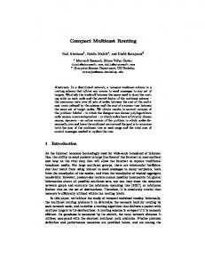
To support real-time multicast, we must first understand real-time switches and their multicast mechanisms. Network switches (no matter real-time or not) can be generally categorized as output queueing or input queueing. In output queueing, input ports (simplified as “inputs” in the following) does not buffer packets. Once a packet enters an input, it is immediately routed to its corresponding output port (simplified as “output” in the following) and buffered there. Though output queueing is simple and intuitive, its inborn “N speed-up” problem1 [14] limits its real-world adoption. Input queueing, instead, becomes the de facto standard among switch vendors. In input queueing, a crossbar fabric connects inputs with outputs (see Fig. 1(a)). Packets are only buffered at inputs; when a packet enters an input, it is immediately routed into the intended queue in the input (see Fig. 1(b)). At scheduled time, an output connects with one input, picks one of its queues, and fetches the queue’s header packet. The fetched packet exits the output directly without further buffering (see Fig. 1(c)). To facilitate scheduling, each packet is typically manipulated as fixed-size (typically 512 bit, and is the same universally) fragments called cells. The time cost to send one cell across the crossbar is called one cell-time. To satisfy the crossbar constraint that at any time instance, an input can connect to at the most one output and vice versa, input switches operate periodically, and the period is one celltime. At the beginning of each cell-time, the switch scheduler decides a one-to-one matching (simplified as “matching” in the following) between inputs and outputs and connect/disconnect crossbar intersections (the grey dots in Fig. 1(a)) accordingly.

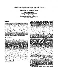
The term “conflict free” means at any slot of the frame, each input is granted by no more than one output, and vice versa. That is, a conflict free schedule is the combined M -slot frame schedules of all N outputs, which dictates a matching between the N inputs and N outputs in each cell-time. Fig. 2 illustrates the meanings of conflict free schedule3 . The above real-time switch design can be easily extended to support multicast (as shown in Fig. 3). When a to-bemulticasted cell enters an input (see Fig. 3 (a)), it is duplicated into m copies (see Fig. 3 (b)), one for each output that it shall multicast to. Each copy enters its corresponding input perflow queue, and the rest is the same as unicast. When the copy enters the next-hop switch, same thing can happen again for further multicasts. Such extension complies with the common constraint of crossbar that at any time instance, one input can connect to at the most one output and vice versa; hence will benefit legacy reuse and smooth design evolution. Note one specialty of the above real-time switch multicast is that output links’ capacities are no longer independent. This is shown by Fig. 4. In the figure, a multicast tree branches to output O1, O2, and O3. The traffic load on O1, O2,

1 For an output queueing switch of N inputs and N outputs, suppose the capacities of all inputs are the same, then inside the switch, the fabric capacity at each output must be N times that of an input’s capacity. This is for the case that all inputs inject traffic to a same output with their full capacities.

2 We can use static schedule because for most real-time applications, such as avionics and industrial control, most flows are for stable and permanent control loops. 3 Interested readers can refer to [16] for the O(N 4 ) scheduling algorithm.

Theorem 1 (Schedulability): For an N × N real-time switch described above, if in every M -slot frame, each output needs to receive no more than M cells, and each input needs to send no more than M cells, then we can always derive a conflict free schedule with a time cost of O(N 4 ).

(a) crossbar fabric, which connects inputs with outputs; each input connects to a data bus (the horizontal line segments) that intersects with each output’s data bus (the vertical line segments); the intersections (grey dots) can be connected/disconnected during runtime by scheduler(s); note at any time, one input can connect to at the most one output, and vice versa.

Fig. 2. Conflict free schedule for real-time switch of [16]: in this example, the switch has N = 4 inputs and outputs, frame size is M = 5 slots (note in reality, M is in the order of 103 ∼ 106 ); each row of the “schedule matrix” is a conflict free schedule for its corresponding output, which means at any time slot (i.e., any column of the “schedule matrix”), no two outputs contend for the same input (for different input queues).

(b) an input port: packet routing and queueing are carried out in it; in input i, the kth queue buffering packets to output j is denoted as Q(i, j, k). (a) Step 1

(c) an output port: at different time slot, the output fetches packets from different input queues according to the switch scheduling scheme. Fig. 1.

Input Queueing Switch Architecture

(b) Step 2 Fig. 3.

Multicast in Real-Time Switch of [16]

Fig. 4. Multiple outputs’ link capacity may be coupled via the shared input during multicast

We can model every multi-hop switched fieldbus as a ~ ~ where V and E ~ are G’s ~ vertex set directed graph G(V, E), and edge set respectively. Every vertex v ∈ V corresponds ~ let src(~e) to a switch in the fieldbus. For every edge ~e ∈ E, and des(~e) denote its source end and destination end vertices respectively. Then ~e represents a physical link that connects an output of switch src(~e) to an input of switch des(~e). We can also denote ~e as hx, yi, where x = src(~e) ∈ V and y = des(~e) ∈ V . Let M represent the set of all real-time multicast groups to be routed. A real-time multicast group m ∈ M is a tuple def of m = (s, D, w, T, H), where s ∈ V is the source end of the multicast, D ⊆ V is the set of destination ends of the multicast. T (cell-time) is the traffic generation period. That is, in every T cell-time, the source end switch s has w cells ready to be multicasted to the group. Note the w cells are released at the exact beginning of each T cell-time period, i.e., there is no jitter in traffic generation at the source end. These w cells must reach all vertices in D within H cell-time. An instance of an RTMS problem can be expressed as a ~ ~ M), who aims to find a feasible schedule tuple q = (G(V, E), ~ ~ so that for each multicast group for every switch in G(V, E), m ∈ M, m’s real-time multicast demand is satisfied. B. RTMS Problem is NP-Hard

and O3 are all 1 cell/frame. But due to the duplication of cells, the upstream input I0 have to schedule 3 cell/frame for the multicast. In an extreme case where M = 2 cell/frame, although none of O1 ∼ O3 reaches its capacity of 2cell/frame, I0 already becomes unschedulable. Also note one common misunderstanding is that the multicast is accomplished by an output connected to multiple next-hop switches. In fact, each output is connected to just ONE input of ONE next-hop switch. The output can create a multicast cell, but the duplication of the cell takes place inside the next-hop input. III. R EAL -T IME M ULTICAST BETWEEN S WITCHES Given individual switch design that supports real-time multicast, we now study how to coordinate these switches for realtime multicast. We can start our discussion from the real-time multicast scheduling (RTMS) problem. A. Real-Time Multicast Scheduling (RTMS) Problem To ease narration, we give the following assumption for this paper (note in the following, our claims on problem complexity still sustain even without this assumption; and we leave the design of real-time multicast under clock skew to our future publications). Assumption 1: In the rest of this paper, we always assume multi-hop switched fieldbuses use the multicast-capable input queueing real-time switch described in Section II. We also assume all switches have the same cell-time duration and the same frame size of M cell-time/frame, a.k.a. M slot/frame.

Before seeking an algorithm for RTMS problem, we are interested in first knowing the problem complexity. We find the following theorem: Theorem 2: RTMS problem is NP-Hard. Proof: Let us first set the following assumption in addition to Assumption 1: Assumption 2 (only used in this proof): We assume all switches are perfectly synchronized, that is, all switches have the same clock phase. With Assumption 2, we can reduce the well-known NPHard problem of Minimum Broadcast Time (MBT) [19] to RTMS problem. For reader’s convenience, MBT problem [19] is re-stated in the following. Definition 1 (MBT Problem): Given a graph G = (V, E), subset V0 ⊆ V , and a positive integer K, can a message be “broadcast” from the base set V0 to all other vertices in K steps. That is, is there a sequence V0 , E1 , V1 , E2 , . . ., EK , VK such that each Vi ⊆ V , each Ei ⊆ E, and for 1 ≤ i ≤ K, (1) each edge in Ei has exactly one end point in Vi−1 , (2) no two edges in Ei share a common end point, and (3) Vi = Vi−1 ∪ {v|hu, vi ∈ Ei }? Our reduction goes as follows. Given an instance of MBT problem, we build an RTMS ~ ′ , E) ~ from the MBT graph G(V, E) through three graph G(V steps: ~ := ∅; i) initially, V ′ := V and E

ii) for every edge e = hu, vi ∈ E, add two directed edges ~ hu, vi and hv, ui into E; iii) if V0 of MBT problem only has one vertex, then denote this vertex as s0 ; otherwise, add a new vertex s0 into V ′ and ~ for each v ∈ V0 . add directed edges hs0 , vi into E The following proof applies to the |V0 | = 1 case; the proof for the |V0 | > 1 case follows the same path, and is left for interested readers for the brevity of analysis. ~ ′ , E), ~ every vertex in V ′ is In our RTMS problem on G(V a multicast-capable input queueing real-time switch described in Section II; and we set the globally consistent frame size M := max{K, |V ′ |}, where K is the broadcast deadline given in the MBT problem, and |V ′ | is the number of elements in set V ′ . Our RTMS problem shall only have one multicast group: m = (s0 , VK , 1, M, K), where as mentioned before, M = max{K, |V ′ |}. That is, in each period of M cell-time, which is also the length of a frame, one cell is generated at s0 ; and this cell must be multicasted from s0 to all the vertices in VK within K cell-time. We claim the above reduction is valid due to the following reasons. First, the reduction apparently takes only polynomial time. Second, our mapped RTMS problem’s solution schedule (if exists) shall satisfy the original MBT problem’s requirement (2). Remember due to Assumption 2, all switches in the fieldbus are perfectly synchronized (0 phase difference), and have the same cell-time and frame duration. Therefore, we can focus on the schedule within just one frame. In each frame, each switch can have at the most one input to be the multicast upstream, i.e., where the singular to-be-multicasted cell c enters. Without loss of generality, let us focus on one such switch and denote its multicast upstream input as I. Then in each cell-time of the frame, at most one output can fetch c from I (due to the feature of crossbar, see Section II). This means no two (out-going) edges of a same vertex (switch) participate multicast in the same cell-time. As all cell-time are globally synchronized, this means MBT problem’s requirement (2) is satisfied (note: view each celltime as a MBT broadcast step). Third, by viewing each cell-time of our RTMS solution schedule as a step, MBT problem’s requirement (1) and (3) are apparently satisfied. Therefore, under Assumption 2, any instance of MBT problem can be reduced (within polynomial time) to an instance of RTMS problem. Therefore, RTMS problem is also NP-Hard. Now, if we remove Assumption 2, RTMS problem becomes more general, and hence more difficult. Therefore, we can claim even without Assumption 2, RTMS problem is still NPHard.  C. Converting RTMS Problem to Real-Time Multicast Routing (RTMR) Problem Due to the NP-Hardness, we cannot find an optimal algorithm for RTMS problem (an optimal algorithm means for any instance of RTMS problem that has solution(s), the algorithm

can always find a solution within polynomial time). Instead, we shall pursue an efficient algorithm that can find a solution in polynomial time for a fairly large number of RTMS problem instances. However, even to design such an efficient algorithm is too difficult. Therefore, we choose to only focus on a RTMS problem subset, whose member multicast groups’ traffic generation periods are always M cell-time, i.e., same as the universal switch scheduling frame size. We call this subset of RTMS problem M -slot Periodic RTMS problem, The above concepts are summarized by the following symbolic notations. Let def

Q = {q|q is an instance of an RTMS problem}

(2)

denote the set of all instances of RTMS problem. Then the set of all instances of M -slot Periodic RTMS problem can be denoted as Q′ : Q′

def

=

~ M) ∈ Q, M = {mi }, {q ′ |q ′ = (G, mi = (si , Di , wi , Ti , Hi ), and ∀i, Ti ≡M },

(3)

where M (cell-time/frame) is the universal switch scheduling frame size. Unfortunately, Q′ is still too difficult. In fact, we have the following proposition: Proposition 1: M -slot Periodic RTMS problem is NPHard. Proof: Same as the proof of Theorem 2.



Therefore, we decide to add some more constraints to further shrink our problem space. Specifically, for each in~ M) ∈ Q′ , where M = {mi }, we construct stance q ′ = (G, ~ M). ˜ G ~ still another instance of problem denoted as q˜ = (G, represents the same multi-hop switch network topology as in ˜ = {m q′ . M ˜ i } is the set of multicast groups in problem q˜, and is constructed from M = {mi } as follows. For each multicast group mi = (si , Di , wi , Ti (≡M ), Hi ) ∈ M, a multicast group ˜ i ) is added to M. ˜ The symbolic m ˜ i = (si , Di , wi , Ti (≡M ), H meanings of si , Di , wi , and Ti (≡M ) are still the same as in mi . However, ˜ i def H = max



  Hi − M ,0 , M +1

(4)

and now means the multicast tree must be NO taller than ˜ i hops. We call the constructed q˜ an instance of real-time H multicast routing (RTMR) problem, and denote the set of all ˜ instances of RTMR problem as Q. We have two observations:

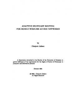
Proposition 2: For a problem instance of ~ ~ {m ˜ if a switch v ∈ V q˜ = (G(V, E), ˜ i }) ∈ Q, participates in the multicast for one multicast group ˜ i ), then in each M -slot m ˜ i = (si , Di , wi , Ti (≡M ), H frame, each of v’s participating output must schedule at least wi slots to fetch (and hence forward) cells for m ˜ i. This proposition also applies to M -slot Periodic RTMS problem. Proof: As the source si generates wi cells per M -slot frame (remember Ti ≡M ), and the real-time switch runs the same TDMA schedule in every M -slot frame, if the output does not schedule at least wi slots per M -slot frame, the queue will overflow and hence cause deadline misses.  Therefore, in designing an efficient algorithm for RTMR problem, we add the following implicit rule: ~ ~ {m Rule 1: For a problem instance of q˜ = (G(V, E), ˜ i }) ∈ ˜ Q, if a switch v ∈ V participates in the multicast for one ˜ i ), then in multicast group m ˜ i = (si , Di , wi , Ti (≡M ), H each M -slot frame, each of v’s participating output must schedule exactly wi slots to fetch (and hence forward) cells for m ˜ i. The other observation is as follows: Proposition 3: If an instance of RTMR problem q˜ is constructed from an instance of M -slot Periodic RTMS problem q ′ through the aforementioned method, then a solution to q˜ is also a solution to q ′ . Proof: Note a solution to q˜ means the end-to-end delay for m ˜ i is bounded by Hi cell-time.  Note the reverse is not necessarily true: a solution to q ′ is not necessarily a solution to q˜. Nonetheless, the above proposition means if an algorithm solves a fairly large number of RTMR problem instances, then it also solves a fairly large number of RTMS problem instances. That is, we can seek an efficient algorithm for RTMR problem as our efficient algorithm for RTMS problem. Besides, RTMR problem itself is also of good practical value, and is mainly about routing, which we are more familiar with. IV. A N E FFICIENT RTMR A LGORITHM Due to the above analysis, we are only interested in finding an efficient heuristic algorithm for RTMR (and hence RTMS) problems. The accurate definition of our heuristic algorithm involves a lot of trivial details. Hence we put it in Appendix A. In this section, we shall only give some high level intuitions. To “grow” (route) a multicast tree for a multicast group, we can either choose “depth first” or “width first”. Without loss of generality, we choose to grow multicast trees in a “depth first” fashion. This is illustrated by Fig. 5. In the figure, the nodes represent real-time switches, which form a network of 4 × 4 grid. The example multicast group roots in node 1, and

Fig. 5.

“Growing” (routing) multicast tree in a “Depth First” fashion

includes destination node 13 and 12. Initially, the tree only includes root node 1, as shown in Fig. 5 (a). Since the closest destination (from existing tree) is node 13, “depth first” routing first “grows” route 1 → 5 → 9 → 13, as shown in Fig. 5 (b). Now the closest destination (from existing tree) is node 12, and the corresponding “branching” node is node 9. So “depth first” routing then “grows” route 9 → 10 → 11 → 12, as shown in Fig. 5 (c). As mentioned before, a fieldbus is a confined system. We can have global information. Besides, fieldbuses are usually configured/reconfigured offline. Therefore, our routing algorithm can be carried out in a centralized way. When there are multiple multicast trees to “grow”, we grow them simultaneously with multiple iterations. In each iteration, one link is added to each tree. Therefore, sometimes multiple trees may contend for outputs and frame time-slots in a same switch. The contention is addressed with a matching algorithm that mimics job-hunting. The intuition of “job-hunting” based matching runs like following. All trees play the role of “applicants” in the “job-hunting”, while all outputs play the role of “employers”. The “jobhunting” runs several iterations until all trees find their preferred outputs and frame time-slots, or declare failure. Each iteration consists of three sequential steps. Step 1 (Apply for Job): Each tree ranks all outputs, and “applies” only to the output that ranks highest. Suppose O is the set of all outputs on the switch; rt,o is the ranking of output o by tree def def t; o(t,1) = argmaxo∈O {rt,o }; and o(t,2) = argmaxo∈O−{o(t,1) } {rt,o }. Then t only applies to o(t,1) . Step 2 (Offer Job): On receiving job application(s), an output o grants the tree who is the most “loyal”, i.e., o shall grant tree t∗ = argmax{t|t applied to o} {rt,o(t,1) − rt,o(t,2) }. Step 3 (Accept Job): If a tree is granted a “job-offer” from Step 2, it accepts the granting output, and reserves on scheduling frame slots accordingly. Note as in Step 1, a tree only applies to ONE output, it can be granted by at the most ONE output in Step 3. More formal details of the “job-hunting” process is described in Fig. 8 of Appendix A. One key element of the above three step “job-hunting” is the calculation of rank in Step 1, as the ranking directly influences

which tree is assigned with which output/route. In our heuristic algorithm, suppose a “growing” tree t attempts to route through an output o on switch u that connects to next hop switch v (i.e. link hu, vi), then t shall rank o as follows: ˜ − H(t, v)) γ o (H rt,o = , (5) dis(v, t.target) ˜ is the maximum tree height limit given by the RTMR where H problem; H(t, v) is the hop count from t’s root to v along the current tree t; t.target is the current depth first routing destination picked by t (e.g., between Fig. 5 (a) to (b), the target is node 13); dis(v, t.target) measures the shortest path hop count between v and t.target in the whole switched network. ˜ − H(t, v)) indicates how much flexibility Therefore, (H ˜ the is left if t picks o. In the extreme case, H(t, v) = H, tree reaches its height upper bound, hence has no flexibility any more. On the other hand, dis(v, t.target) add preference to outputs that lead the tree closer to the intended target destination. The more complicated parameter in Equation (5) is γo . It evaluates the expected congestion increase on switch u (the switch that o belongs to) if the tree t chooses output o:  1 (if maxj∈Ou {Nj }     = maxj∈Ou {Nj′ }), γo = , (6)  exp(maxj∈Ou {Nj } (otherwise)    − maxj∈Ou {Nj′ })

where Ou is the set of all outputs of switch u; Nj is the number of reserved slots of output j’s M -slot frame schedule; and Nj′ is the number of reserved slots of output j’s M -slot frame schedule if tree t finally decides to route through output o. Combining all above, Equation (5) reflects our heuristic of routing preference on a path that is least congested, minimally increases tree height, and leads closer to target destinations. We have the following propositions: Proposition 4: If K trees participate the “job-hunting”-like edge/output-port assignment depicted in the pseudo code of Fig. 8, then the process terminates in at the most K iterations. Proof: Due to line 19 of the pseudo code, the iteration will terminate unless line 25 is executed, which implies line 24 is executed, which implies at least one tree finds its matching and is removed from the “applicant” set (A in Fig. 8). As there are K (i.e., |A| = K) trees, there can be at the most K iterations.  Proposition 5: Our heuristic algorithm terminates in polynomial time. Proof: Due to Proposition 4 and the pseudo code presented in Appendix A. 

Note, as fieldbus routing is planned offline, we leave the more detailed algorithm time complexity analysis to interested readers. V. E VALUATION In the Internet literature, the best known multicast algorithms are Distance Vector Multicast Routing Protocol (DVMRP) [20] and Multicast Extension to Open Shortest Path First (MOSPF) [21][22]. However, under optimal conditions, i.e., the network is static, and all nodes have accurate global information, DVMRP and MOSPF both produce the shortest path tree for the multicast group, using the well-known Dijkstra algorithm [23]. Therefore, we shall compare our RTMR heuristic algorithm with Dijkstra algorithm. Our comparisons are based on simulations. In our simulation, we assume a multihop switched industrial fieldbus with a two-dimensional 12 × 12 switches grid topology. Each switch has a per port capacity of 1Gbps. Without loss of generality, we assume cell size is 500bit/cell; and M = 2000 cell/frame. We generate typical real-time video and sensing/actuation multicast traffic [15] with uniform multicast destinations distribution. Our results show that our RTMR heuristics algorithm achieves a 21% gain on acceptable (i.e., with a routing success rate of over 50%) network utilization demand compared to Dijkstra. More detailed simulation results are to be published in the journal version of this paper due to page limits. VI. R ELATED W ORK Although multicast is not widely supported in the Internet, many multicast schemes are proposed. Such as Reverse Path Broadcasting/Multicasting (RPB/RPM) [24], Truncated Reverse Path Broadcasting (TRPB) [24], Distance Vector Multicast Routing Protocol (DVMRP) [20], Multicast Extension to Open Shortest Path First (MOSPF) [21][22], ProtocolIndependent Multicast (PIM) [25][26], Core-Based Tree Multicast Routing (CBT) [27], and more recently on overlay P2P network multicasting [28][29]. Most Internet multicast routing protocols are to deal with group management in the multicast tree. This is because of the high dynamics of Internet: nodes join/leave multicast groups frequently. Meanwhile, due to the enormous scale of Internet, it is hard to maintain a global view, hence group management must be distributed. Dynamic and distributed group management, however, is not fieldbus multicast routing’s major concern. As a fieldbus is a specialized confined network, we can have global information. Meanwhile, most fieldbus traffic is for periodical sensing/actuating. Such traffic is typically stable and consistent. Changes mainly take place offline during plant reconfigurations. Therefore, we do not have to make the routing algorithm as fast as online algorithms. P2P and overlay network multicast are concerned with statistical performance. Fieldbus multicast, on the other hand, is hard real-time: every deadline must be caught, otherwise major failure may happen.

VII. C ONCLUSION We proved that the Real-Time Multicast Scheduling (RTMS) problem on multi-hop switched fieldbuses is NPHard. To devise an efficient algorithm for RTMS, we transform instances of RTMS problem to instances of Real-Time Multicast Routing (RTMR) problem. We devised a heuristic algorithm that takes into consideration of both link congestion and real-time end-to-end deadline requirements. Simulation results show that our heuristic RTMR algorithm achieves higher routing success rate under high network utilization demand than main-stream multicast algorithm. ACKNOWLEDGEMENT The project related to this paper is supported in part by NSERC Discovery Grant 341823-07, NSERC Strategic Grant STPGP 364910-08, FQRNT grant 2010-NC-131844, CFI Leaders Opportunity Fund 23090, The Hong Kong Polytechnic University (HK PolyU) Internal Competitive Research Grant (DA) A-PJ68, HK PolyU Newly Recruited Junior Academic Staff Grant A-PJ80, HK PolyU Fund for CERG Project Rated 3.5 (DA) grant A-PK46. Dr. Qixin Wang is also funded by Department of Computing start up fund. Mr. Yufei Wang is also supported by HK PolyU FTE fund. Any opinions, findings, and conclusions or recommendations expressed in this publication are those of the authors and do not necessarily reflect the views of sponsors. The authors thank anonymous reviewers for their advice on improving this paper. R EFERENCES [1] Wayne Wolf, “Cyber-physical systems,” IEEE Computer, vol. 42, no. 3, 2009. [2] Edward Lee, “Cyber-physical systems: Design challenges,” Proc. of International Symposium on Object/Component/Service-Oriented RealTime Distributed Computing (ISORC), May 2008. [3] PCAST, Federal Networking and Information technology R&D (NITRD) Program Review, 2007. [4] Fieldbus Foundation. http://www.fieldbus.org. [5] CAN in Automation. http://www.can-cia.org. [6] PI-PROFIBUS & PROFINET International. http://www.profibus.com. [7] Avionics Databus Solutions. http://www.afdx.com. [8] IEEE Standard 1588-2008, 2008. [9] Qing-Long Han, “A new delay-dependent absolute stability criterion for a class of nonlinear neutral systems,” Automatica, vol. 44, no. 1, pp. 272–277, Jan. 2008. [10] Hongbo Li, Zengqi Sun, Mo-Yuen Chow, Huaping Liu, and Badong Chen, “Stabilization of networked control systems with time delay and packet dropout – part ii,” Proc. of IEEE Inernational Conf. on Automation and Logistics, Aug. 2007. [11] Mo-Yuen Chow and Yodyium Tipsuwan, “Network-based control systems: A tutorial,” Proc. of the 27th Annual Conf. of the IEEE Industrial Electronics Society (IECON’01), 2001. [12] Karl J. Astrom and Bjorn Wittenmark, Computer-Controlled Systems: Theory and Design (3rd Ed.). Prentice Hall, Nov. 1996. [13] Gene F. Franklin, J. David Powell, and Abbas Emami-Naeini, Feedback Control of Dynamic Systems. Addison-Wesley Publishing Company, Nov. 1993. [14] Sathish Gopalakrishnan, Marco Caccamo, and Lui Sha, “Switch scheduling and network design for real-time systems,” in Proc. of IEEE RTAS 2006, Apr. 2006. [15] Qixin Wang and Sathish Gopalakrishnan, “Adapting a main-stream internet switch architecture for multi-hop real-time industrial networks,” IEEE Transactions on Industrial Informatics, vol. 6, no. 3, pp. 393–404, 2010.

[16] Qixin Wang, Sathish Gopalakrishnan, Xue Liu, and Lui Sha, “A switch design for real-time industrial networks,” in Proc. of IEEE RTAS 2008, Apr. 2008, pp. 367–376. [17] F. Dopatka and R. Wismuller, “Design of a realtime industrial ethernet network including hot-pluggable asynchronous devices,” IEEE International Symposium on Industrial Electronics (ISIE 2007), 2007. [18] Yiu-Wing Leung and Tak-Shing Yum, “A TDM-based multibus packet switch,” IEEE Trans. on Communications, vol. 45, no. 7, pp. 859–866, Jul. 1997. [19] Michael R. Garey and David S. Johnson, Computers and Intractability: A Guide to the Theory of NP-Completeness. W. H. Freeman and Company, 1979. [20] D. Waitzman, C. Partridge, and S. Deering, Distance Vector Multicast Routing Protocol. RFC 1075, Nov. 1988. [21] John Moy, Multicast Extensions to OSPF. RFC 1584, Mar. 1994. [22] ——, MOSPF: Analysis and Experience. RFC 1585, Mar. 1994. [23] Gary Chartrand, Introductory Graph Theory. Dover Publications, Dec. 1984. [24] Chuck Semeria and Tom Maufer, Introduction to IP Multicast Routing. IETF draft-ietf-mboned-intro-multicast-03.txt, Jul. 1997. [25] B. Fenner, M. Handley, H. Holbrook, and I. Kouvelas, Protocol Independent Multicast – Sparse Mode (PIM-SM): Protocol Specification (Revised). RFC 4601, Aug. 2006. [26] A. Adams, J. Nicholas, and W. Siadak, Protocol Independent Multicast – Dense Mode (PIM-DM): Protocol Specification (Revised). RFC 3973, Jan. 2005. [27] A. Ballardie, Core Based Trees (CBT) Multicast Routing Architecture. RFC 2201, Sep. 1997. [28] Yang-hua Chu, Sanjay G. Rao, Srinivasan Seshan, and Hui Zhang, “A case for end system multicast,” ACM SIGMETRICS, 2000. [29] Xiaowen Chu, Kaiyong Zhao, Zongpeng Li, and Anirban Mahanti, “Auction-based on-demand p2p min-cost media streaming with network coding,” IEEE Transactions on Parallel and Distributed Systems, vol. 20, no. 12, Dec. 2009.

A PPENDIX A RTMR A LGORITHM P SEUDO C ODE In the following, we give the pseudo code of our heuristic RTMR algorithm. ~ ~ and the set We assume the switched fieldbus graph G(V, E) ˜ = {m ˜ i )} are of all multicast groups M ˜ i = (si , Di , wi , M, H given global variables. For convenience, we use the following data structures: We use tuple t = (A, B, m, ˜ a, d, G) to represent a multicast tree for multicast group m. ˜ A is t’s vertex set; B is t’s edge set; m ˜ is the corresponding multicast group; a is the current growing vertex (explained later); d is the current routing target (explained later); and G is a temporary data structure only used in function AssignEdges (see Fig. 8), representing the set of all candidate (a.k.a. granting) outputs for next hop routing. In addition, A, B, m, ˜ a, d, and G are accessible through t.vertex set, t.edge set, t.multicast group, t.vertex to grow, t.cur target, and t.granting outputs respectively. Before our program starts, for each multicast ˜ we initiate m group m ˜ i ∈ M, ˜ i ’s multicast tree ti := ({si }, ∅, m ˜ i , si , null, ∅), i.e., ti .vertex set = {si }, ti .edge set = ∅, ti .multicast group = m ˜ i, ti .vertex to grow = si , ti .cur target = null, ti .granting outputs = ∅.

We use tuple v = (I, O, A) to denote every vertex v ∈ V . Each vertex in V represents an aforementioned real-time switch. I and O are vertex/switch v’s input set and output set respectively. A is a temporary data structure only used in

function AssignEdges (see Fig. 8), representing the set of trees that want to route through this vertex/switch. In addition, I, O, and A are accessible via v.input ports, v.output ports, and v.applicant trees. With the above conventions, Fig. 6 shows the pseudo code of our main program. ~ ~ and M ˜ = {m ˜ i )} // Note G(V, E) ˜ i = (si , Di , wi , M, H // are given global variables 1. main function RTMR() ˜ or find a routing tree ti for 2. result: either claim unable to solve M; each m ˜ i , such that ti ’s root is si , ti ’s leaves are Di , ti is a subgraph ~ every vertex (switch) in ti is schedulable, and ti ’s height is of G, ˜ i hops. no taller than H 3. { ˜ 4. Let the set of all successfully routed (grown) multicast S trees T := ∅; 5. Let the set of all to-be-grown multicast trees T := {ti }; 6. while (T = 6 ∅) { 7. foreach v ∈ V , set v.applicant trees := ∅; 8. foreach ti ∈ T { 9. UpdateVertexToGrow(ti ); 10. Let v := ti .vertex to grow; ˜ 11. if (v = null) return claim unable to solve M; S 12. else v.applicant trees := v.applicant trees {ti }; 13. } 14. foreach (v ∈ V and v.applicant trees 6= ∅) { 15. boolean result := AssignEdges(v); 16. if (result = true) { 17. ∆ := {δ ∈ v.applicant trees|δ reached all intended multicast destinations}; S 18. T˜ := T˜ ∆; T := T − ∆; ˜ 19. }else return claim unable to solve M; 20. } 21. } 22. return the routed trees T˜ ; 23. } Fig. 6.

Main Function for RTMR

Fig. 7 describes the UpdateVertexToGrow function of the main program. UpdateVertexToGrow plays the main role in carrying out the “depth first” tree growth strategy. 1. function UpdateVertexToGrow(t) 2. result: update t.vertex to grow; or set t.vertex to grow := null if failed to find feasible vertex to grow; 3. { ˜ := t.multicast group; 4. denote m ˜ = (s, D, w, M, H) 5. if (t.cur target = null or t has reached t.cur target) { 6. Let D ′ := D − t.vertex set, that is, D ′ is the remaining destinations of m ˜ that t has not yet reached; 7. Choose a′ ∈ t.vertex set and d′ ∈ D ′ such that ∀x ∈ t.vertex set and ∀y ∈ D ′ , dis(x, y) ≥ dis(a′ , d′ ), where dis(x, y) is the shortest hop count from vertex x to y ~ in graph G; 8. if (a′ ’s input can schedule a new branch of t toward d′ ) { 9. t.vertex to grow := a′ ; 10. t.target := d′ ; 11. }else t.vertex to grow := null; //return failure 12. } //else do nothing 13. } Fig. 7.

UpdateVertexToGrow Function for RTMR

Fig. 8 describes the AssignEdges function in the main program. This function carries out the “job-hunting”-like tree

routing contention resolution mechanisms. 1. function AssignEdges(v) 2. result: if successfully assigns each applicant tree an output link (i.e. each tree grows), return true; otherwise, claim failure to find feasible route by returning false. 3. { 4. Let O := v.output ports; //analogy: set of employers 5. Let A := v.applicant trees; //analogy: set of applicants 6. foreach t ∈ A, set t.granting outputs := ∅; 7. boolean inf easible := false; 8. while (A 6= ∅ and not inf easible) { //analogy: another iteration of job-hunting starts 9. ∀t ∈ A and ∀o ∈ O, let rt,o :=Ranking(t, o); 10. o(t,1) := argmaxo∈O {rt,o }; 11. o(t,2) := argmaxo∈O−{o(t,1) } {rt,o }; //analogy: all applicants rank all employers; and apply only to o(t,1) . //rt,o indicates how much t prefers o as its next hop. 12. foreach (o ∈ O) { 13. Choose t∗ := argmax{t|t∈A and o=o(t,1) } {rt,o(t,1) − rt,o(t,2) }; ˜ 14. Suppose t∗ .multicast group = (s, D, w, M, H); 15. if (rt∗ ,o ≥ 0 ){ //o is feasible for t∗ S 16. t∗ .granting outputs := t∗ .granting outputs {o}; //analogy: employer o offers job to the most loyal applicant 17. } 18. } 19. inf easible := true; 20. foreach (t ∈ A) { 21. Denote G = t.granting outputs; 22. if (G = 6 ∅) { 23. t accepts o∗ = o(t,1) ’s grant, i.e., t choose o∗ as the next step output, reserves proper slots on o∗ ’s and corresponding input’s schedule, and update t’s corresponding internal data structures; //analogy: t accepts the best job offer 24. A := A − {t}; 25. inf easible := false; //may have more possible matches 26. } 27. } 28. } 29. if (A 6= ∅ and inf easible) return false; 30. else return true; 31. } Fig. 8.

AssignEdges Function for RTMR

Fig. 9 is the Ranking function called in function AssignEdges. 1. function Ranking(t, o) 2. result: a non-negative number indicating tree t’s preference on choosing output o as its next hop, the larger the more preferable; or −1 if choosing o is infeasible. 3. { ˜ := t.multicast group; 4. Let m ˜ = {s, D, w, M, H} ˜ 5. if (choosing o as next hop output makes t’s height exceed H) return −1; 6. if (o cannot schedule t’s traffic of w cell/frame) return −1; 7. if (in case of multicast branching, the corresponding input cannot schedule additional w cell/frame of t’s traffic) return −1; 8. return ranking calculated per Equation (5) of Section IV; 9. } Fig. 9.

Ranking Function for RTMR