Int. J. Sensor Networks, Vol. 15, No. 2, 2014
95
A real-time routing protocol with mobility support and load distribution for mobile wireless sensor networks Adel A. Ahmed* Faculty of Computing and Information Technology, King Abdulaziz University, Rabigh 21911, KSA E-mail:
[email protected] *Corresponding author
Norsheila Fisal Faculty of Electrical, Telecommunication Department, University Technology Malaysia, Skudai, Malaysia E-mail:
[email protected] Abstract: Mobile wireless sensor network (MWSN) is a wireless ad hoc network that consists of a very large number of tiny sensor nodes communicating with each other in which sensor nodes are either equipped with motors for active mobility or attached to mobile objects for passive mobility. A real-time routing protocol for MWSN is an exciting area of research because messages are delivered according to their end-to-end deadlines. MWSN demands real-time routing in many applications including disasters fighting, forest fire detection and volcanic eruption detection. This paper proposes a novel idea of real-time that provides mobility and load distribution (RTMLD) for MWSN. RTMLD utilised corona mechanism and optimal forwarding metrics to forward the data packet in MWSN. It computes the optimal forwarding node based on RSSI, remaining battery level of sensor nodes and packet delay over one-hop. RTMLD ensures high packet delivery ratio and experiences minimum end-to-end delay in WSN and MWSN compared with baseline routing protocol. RTMLD has been successfully verified through test bed and simulation experiment. Keywords: mobile sensor node; corona mechanism; sensor networks; remaining power; end-to-end packet delay. Reference to this paper should be made as follows: Ahmed, A.A. and Fisal, N. (2014) ‘A real-time routing protocol with mobility support and load distribution for mobile wireless sensor networks’, Int. J. Sensor Networks, Vol. 15, No. 2, pp.95–111. Biographical notes: Adel Ali Ahmed received his BSc in Computer Engineering from Cairo University, Egypt in 2001. He received his MSc and PhD in Telecommunication from University of Technology Malaysia, Malaysia in 2005 and 2008, respectively. He did his Post Doctoral in underground wireless sensor network at University Technology Malaysia 2008. Currently, he is an Assistant Professor at King Abdulaziz University, Rabigh, Saudi Arabia. He is interesting in MANET, mobile WSN, location tracking, security and distributed systems in WSN, and underground WSN. He published many journal and conference papers and he worked reviewer and technical committee in some conferences. Norsheila Fisal received her BSc in Electronic Communication from the University of Salford, Manchester, UK in 1984. MSc in Telecommunication Technology, and PhD in Data Communication from the University of Aston, Birmingham, UK in 1986 and 1993, respectively. Currently, she is the Professor with the Faculty of Electrical Engineering, University Technology Malaysia and Director of Telematic Research Group (TRG) Laboratory.
Copyright © 2014 Inderscience Enterprises Ltd.
96
1
A.A. Ahmed and N. Fisal
Introduction
Wireless sensor network (WSN) may consist of a large number of sensor nodes, which are densely deployed in close proximity to the phenomenon. In WSN, sensors gather information about the physical world and the base station or the sink node makes decision and performs appropriate actions on the environment (Akyildiz et al., 2002; Song et al., 2008). A MWSN can be considered as a collection of distributed sensor nodes, which are capable of sensing, moving, communicating within its allowable range. The complete system architecture of a MWSN includes a group of mobile and static sensor nodes, a mobile base station (laptop or PDA), and upper communication network infrastructures. As shown in Figure 1, the sensor nodes are scattered in the target environment and they form a multi-hop mesh networking architecture. Each of these sensor nodes has the capability of collecting data and routing data peer-to-peer to base stations. The mobile sensor node is in fact an enhanced sensor node. It not only has all the capabilities of the static sensor node, but also realises mobility by adding a robotic base and a driver board. Each mobile sensor node is capable of navigating autonomously or under control of humans. Large numbers of mobile sensor nodes can coordinate their actions through ad hoc communication networks. A base station or mobile sink is used to bridge the sensor network to another network or platform, such as the internet. Mobile sinks offer many benefits to the network. For instance, they help to improve scalability, maintain load balance, conserve energy and prolong network lifetime (Song et al., 2008; Indu et al., 2010). MWSN is very different from traditional networks as it comprises of a large number of nodes that produce a very large amount of data. However, MWSNs are not free of certain constraints such as power, computational capacities and memory. Figure 1
MWSN architecture (see online version for colours)
Moreover, MWSNs are very data-centric, meaning that the information that has been collected about an environment must be delivered in a timely fashion to a collecting agent or mobile sink. Since a large number of
sensor nodes are deployed, neighbour nodes may be very close to each other. Hence, multi-hop routing idea is suitable for MWSN to enable channel reuse in different regions of MWSN and overcome some of the signal propagation effects experienced in long-distance wireless communication (Seada et al., 2004; Chen et al., 2007). Routing Protocols for MWSN is a greater challenge than routing in a WSN due to the following reasons. First, since it is not easy to grasp the whole network topology, it is hard to find a routing path. Secondly, sensor nodes are tightly constrained in terms of energy, processing and storage capacities. Thus, to increase the overall lifetime of MWSN, effective resource management policies and especially efficient energy management are required. Real-time communication is necessary for many MWSN applications. For example, in a fire-fighting application where appropriate actions should be made to the event area immediately as delay may cause some huge damages further. The sensor data collected and delivered must still be valid at the time of decision making since late delivery of data may endanger the fire fighter’s life. Without loss of generality, QoS on the real-time guarantee can be categorised into two classes: hard real-time and soft real-time. In hard real-time system, deterministic end-to-end delay bound should be supported. The arrival of a message after its deadline is considered as a failure of the whole system. While in soft real-time system, probabilistic guarantee can meet requirements and some lateness is tolerable. Hence, supporting real-time in MWSNs means there should be either a deterministic or probabilistic end-to-end delay guarantee. It should be noted that while considering real-time support in MWSNs, energy efficiency should not be ignored (Li et al., 2007; Zhan et al., 2008). This paper reports the following main contributions. First, it proposes a real-time maintain mobility with load distribution (RTMLD) routing protocol for MWSN. RTMLD utilises a corona mechanism as a replacement of location-based routing and computes optimal forwarding node based on received signal strength indicator (RSSI), remaining power of sensor nodes and packet velocity over one-hop. Since forwarding nodes with the best link quality are chosen, the data throughput is improved. By choosing the forwarding nodes with the maximum packet velocity, the real-time packet transfer is ensured in the MWSN. Additionally, choosing nodes with the highest remaining power level ensures sporadic selection of forwarding neighbour nodes. The continuous selection of such nodes spread out the traffic load to neighbours in the direction of the sink, and subsequently prolonging the WSN lifetime. RTMLD reports high performance in terms of delivery ratio, end-to-end delay, and power consumption. It has been successfully studied and verified through the real test bed using TelosB motes and simulation experiment using network simulator-2 (NS-2). Secondly, it proposes a mobility detection mechanism that used corona architecture based on the position of the mobile sink (MS). Corona architecture divides MWSN area into a dynamic corona based on a MS which is assumed to be in the centre
A real-time routing protocol with mobility support and load distribution for mobile wireless sensor networks of coronas (Ferng et al., 2011) as it will be explained in Section 3. The rest of this paper is organised as follows: Section 2 will present related work on real-time communication for MWSN. The design of RTMLD will be described in Sections 3 and 4 will describe the simulation study of RTMLD. Section 5 will describe the test bed implementation. Finally Section 6 will conclude the paper.
2
Related work
While most existing WSN deployments are still terrestrial networks with static sensor nodes, mobile wireless sensor networks (MWSNs) have received increasing attention. During the past few years, several MWSNs have been successfully deployed in which sensor nodes are either equipped with motors for active mobility or attached to mobile objects for passive mobility. For example, researchers have attached wireless sensor devices to micro air vehicles (Allred et al., 2007), bikes (Shane et al., 2009), vehicles (Eriksson et al., 2008; Bret et al., 2006) and animals (Wark et al., 2007; Liu et al., 2004). In addition, wireless sensors are equipped with motors to move underwater to collect data from static sensor devices (Vasilescu et al., 2005). The related research for this paper can be classified into two categories as describes as follows.
2.1 Real-time routing protocol for static WSN MM-SPEED is an extension to SPEED protocol (Felemban et al., 2005). It was designed to support multiple communication speeds and provides differentiated reliability. Scheduling messages with deadlines focuses on the problem of providing timeliness guarantees for multi-hop transmissions in a real-time robotic sensor application (Li et al., 2005). In such application, each message is associated with a deadline and may need to traverse multiple hops from the source to the destination. Message’s deadlines are derived from the validity of the accompanying sensor data and the start time of the consuming task at the destination. The authors propose heuristics for online scheduling of messages with deadline constraints as follow: schedules messages based on their per-hop timeliness constraints, carefully exploit spatial reuse of the wireless channel and explicitly avoid collisions to reduce deadline misses. A routing protocol called real-time power control (RTPC) uses velocity with the most energy-efficient forwarding choice as the metrics for selecting a forwarding node (Chipara et al., 2006). A key feature of RTPC is its ability to send the data while adapting to the power of transmission. Ahmed et al. proposed real-time with load distribution (RTLD) for WSN. RTLD computes the optimal forwarding node based on the packet reception rate (PRR), remaining power of sensor nodes and packet velocity over one-hop. It consists of four functional modules that include location
97
management, routing management, power management and neighbourhood management. The location management in each sensor node calculates its location based on the distance to three pre-determined neighbour nodes. RTLD reports high performance in terms of delivery ratio, control packet overhead and power consumption. However, RTPC, MM-SPEED and RTLD are designed for static WSN and unsuitable for MWSN.
2.2 Real-time routing protocol for MWSN Lee et al. proposed an expected area-based real-time (EAR2) routing protocol in WSNs (Lee et al., 2011; Park et al., 2010). EAR2 is based on an expect area (EA) of the mobile sink and exploit flooding of real-time data within EA. It exploits multicasting and one-hop forwarding time. To support a real-time data with a desired time deadline, EAR2 guarantees that the Tset_deadline is smaller than the total summation of the unicast forwarding time from a source to the closest point (CP) of expect zone (EZ) of the mobile sink, the multicast forwarding time from the CP to the grid header of expect grids (EGs), and the one-hop forwarding time from the grid head of an EG to the mobile sink. However, the proposed routing in (Lee et al., 2011; Park et al., 2010) has some constraints such as mobility only applied for a sink and power consumption is high due to multicast data packet to EZ of mobile sink. Araújo et al. proposed routing protocol called RACE which is a network conditions aware geographical forwarding protocol for real-time applications in MWSN (Araújo and Becker, 2011). RACE aims to provide QoS requirements to the application layer by giving priority to real-time messages and also by handling network congestions. Routing is performed node-by-node, where each node calculates a score to choose the best node to forward the message. The score consists of the link quality, the buffer remaining, and the packet velocity. The main feature of RACE is to consider network conditions for calculating the score and has a mechanism to keep knowledge of the buffer situation from the transmitting node to the sink node. Such mechanism provided a considerable improvement in the packet delivery ratio. Simulation experiments show that RACE presents excellent performance in respect to a message delivery ratio and deadline miss ratio. RACE was compared with a wellknown protocol which is real-time power-aware routing (RPAR) and observed that it outperformed RPAR in both metrics. However, RACE is location based and assumed the sink node was static and their positions were previously known. In addition, RACE did not consider load distribution. Keally et al. (2009) proposed Sidewinder, a predictive data forwarding protocol for MWSNs. Like a heat-seeking missile, data packets are guided towards a sink node with increasing accuracy as packets approach the sink. Different from conventional sensor network routing protocols, Sidewinder continuously predicts the current sink location based on distributed knowledge of sink mobility
98
A.A. Ahmed and N. Fisal
among nodes in a multi-hop routing process. Moreover, the continuous sink estimation is scaled and adjusted to performing with resource-constrained wireless sensors. In addition, the authors show the impact of radio ranges on topology changes when nodes are mobile, concluding that traditional mobile ad hoc routing protocols do not work well for MWSN. Moreover, the authors give test bed evidence that geographic forwarding-based protocols in MWSN (forwarding based on sensor node location) have poor performance in terms of delivery ratio and end-to-end delay. This is mainly due to geographical forwarding-based protocols have been widely used in static WSNs, because they only maintain local information to achieve end-to-end routing. However, a common assumption of these geographic forwarding-based protocols is that all intermediate nodes in a routing path know the exact sink location and use it for multi-hop routing. This assumption is reasonable when the sink is static, but leads to poor performance when the sink is mobile. However, Sidewinder does not design for real-time forwarding which required end-to-end delay enhancement to achieve this goal. Singh et al. (2010) proposed tree-based routing protocol (TBRP) with degree constraint for MWSN. TBRP worked in three phases: Tree formation phase, data collection and transmission phase and finally purification phase. TBRP protocol improves nodes and network life time by moving the node to the next higher level. Simulation results show that the nodes at level 0 consume more energy than at higher levels. When these nodes at a lower level reach a critical level of energy, they move to the next higher level, where energy consumption is less thus improving the lifetime of the nodes and network. Simulation results also show that because of mobility in TBRP energy dissipation is more efficient. However, if nodes in the network die (especially parent nodes in a TBRP, where a ‘funnel’ effect results in nodes closest to the base station expending more power more quickly than nodes further from it), the overall coverage and sensing capability of the network will be degraded. A colour theory-based routing protocol by Shee et al. (2005). This protocol works in three phases. This protocol is based on the colour of the geographical area. In this protocol a colour theory-based localisation algorithm is used to find the position of the sensor node. There are various localisation algorithms such as Monte Carlo localisation algorithm (Hu and Evans, 2004; Baggio and Langendoen, 2008) which are used for the localisation of the sensor nodes. However, location-based algorithms are unsuitable for MWSN because they provided poor performance in terms of delivery ratio and end-to-end delay MWSN. RTMLD has the following advantages. First, it utilised corona mechanism rather than location management to deliver the data packet to the MS. Secondly, it maintained corona structure using corona discovery. Thirdly, it utilised the backward corona mechanism to solve the hole routing problem and to produce more flexibility of forwarding.
Fourthly, it simplified optimal calculation equations because RSSI and battery level are measured. Fifthly, RTMLD routing protocol considered mobility in MSN and MS. Finally, RTMLD with application code is small (29662 bytes in ROM; 3000 bytes in RAM) at the memory and suitable for tiny devices such as smart mobile phone.
3
Design of RTMLD
RTMLD is based on our previous routing protocol which is RTLD (Ahmed and Fisal, 2008). The differences between RTLD and RTMLD are as follows: •
Sensor location management: RTLD is depending on location management which calculates the location of a sensor node based on the distance to three pre-determined neighbour nodes. However, geographic forwarding-based is suitable for static WSN and leads to poor performance when the sink and/or intermediate nodes are mobile. Hence RTMLD used corona mechanism as a replacement for location management.
•
Optimal neighbour selection: RTLD computes optimal forwarding node based on the PRR, remaining power of sensor nodes and packet velocity over one-hop. PRR reflects the diverse link qualities within the transmission range and approximately calculated as the probability of successfully receiving a packet between two neighbour nodes (Zuniga and Krishnamachari, 2004). If PRR is high that means the link quality is high and vice versa. However, PRR requires extra time, more energy and complexity mathematical calculation based on IEEE 802.15.4/Zigbee RF transceiver. Hence, RTMLD saves calculation time by utilising RSSI which is a built-in physical layer parameter and does not require any additional calculation.
•
Routing problem handler: in RTMLD, if a mobile sensor node cannot forward data packets to the next-hop neighbour, it backwards a data packet to any node in high corona level and it will inform its parent to stop sending data. This mechanism is called backward corona mechanism. This routing flexibility is not founded on RTLD.
In Figure 2, RTMLD consists of four functional modules that include corona mechanism, routing management, power management and neighbourhood management. The corona mechanism in each sensor node calculates its corona based on the distance to the sink. The power management determines the state of the transceiver and the transmission power of the sensor node. The neighbourhood management discovers a subset of forwarding candidate nodes and maintains a neighbour table of the forwarding candidate nodes. The routing management computes the optimal forwarding choice, makes a forwarding decision and implements a routing problem handler.
A real-time routing protocol with mobility support and load distribution for mobile wireless sensor networks Figure 2
Block diagram of the RTMLD routing protocol
99
shows the forwarding of data packet from mobile sensor node (MSN) to MS. The data travels from MSN that is at a high level of corona to MSN in low levels of the corona. In case MSN does not have any candidate in the neighbour table with low level corona, data packet will be forwarded to MSN that has the same value of the corona. Figure 3
Corona mechanism in MWSN: (a) MWSN model using coronas concentric to MS and (b) MWSN coordinate system after MS travelled (see online version for colours)
3.1 Corona mechanism In corona structure, the whole network is divided into coronas centred on the sink. On the basis of the corona width/radius, the corona model can be classified into uniform-width and non-uniform width corona models. If a uniform width/radius is employed, it is referred to as a uniform width corona (Ferng et al., 2011). The uniform corona model is considered in this paper and simply called corona mechanism for simplicity. It is interested to note that corona structure is similar to tree-based structure. However, the proposed corona mechanism has more flexibility to connect with parents or child this will allow MSN to connect to any child without going through the parent. In addition, to determine corona ID (C_ID) for all sensor nodes in MWSN, MS can broadcast corona control packet (CCP) periodically to one hop neighbours which they will forward CCP again to their neighbours. Figure 3 features MWSN immediately after deployment in which MS is assumed to be in the middle of MWSN. Corona is a concentric circle at the sink. For the sake of simplicity, it is assumed that the corona width is equal to the sensor transmission range r, and hence the radius ri of corona Ci is equal to r × i. The main task of corona mechanism is to imposing a coordinate system of MWSN in such a way that each sensor belongs to exactly one corona (the identity of the corona in which it lies) as illustrated in Figure 3(a). From the experimental work, we found that the optimal coverage distance between two TelosB sensor nodes is 25 m with stable link connection. To maintain corona structure, MS sends CCP every 8 s because if we assume the speed of MSN is between 1 m/s and 5 m/s, and MSN is in the middle between Ci and Ci+1 so MSN will traverse between coronas with 2.5–12.5 s. Therefore, the average is 7.5 s and MSN will send CCP every 8 s. If MSN does not obtain C_ID, it will invoke corona discovery as will be explained below. It is interested to know that MS has enough power to broadcast CCP because it is connected to the laptop or PDA using USB so it has two optional sources of power which are its own battery and laptop or PDA battery. Since MS can travel to any random position, the coordinate system of MWSN and the C_ID of sensor nodes are changed accordingly. As shown in Figure 3(b), MS moves to the left down coroner so the C_ID for sensor nodes is change based on position of MS. Figure 3(b) also
(a)
(b)
3.1.1 Corona discovery Corona discovery is an essential part in the proposed mechanism because it is required in routing management. In the normal case; MS broadcasts CCP which has C_ID to all one hop neighbours. Any MSN receives CCP; it will increase C_ID by one; adjust its C_ID and rebroadcast the CCP again. If MSN receives same CCP, it will discard it. This procedure will be repeated until most MSN obtains C_ID. If any MSN does not obtain C_ID (or MSN has C_ID but it is travelling) and received neighbour discovery request for data forwarding, the corona discovery is invoked. In this discovery, MSN will broadcast C_ID request to all one hop neighbours which will reply with their
100
A.A. Ahmed and N. Fisal
C_ID as illustrated in Figure 4. Upon MSN receives replies, it will calculate C_ID as a roundup average of receiving C_ID in the replies. In Figure 4, MSN H and M did not obtain C_ID and they will send C_ID request. After receiving replies, C_ID of H and M are 5 and 4, respectively. The flowchart diagram of corona mechanism is depicted in Figure 5. In this figure, corona mechanism starts at the MS which will broadcast CCP to all one-hop neighbours. Figure 4
Corona discovery in RTMLD (see online version for colours)
The main fields in the CCP are C_ID (initial value is 0) and CCP_ID. If MSN receives CCP, it will fetch CCP_ID and C_ID. Then, MSN will check CCP_ID whether it has already received the CCP or not. If it has received CCP, MSN will discard this CCP. On the other hand, if CCP has not been received, MSN will increase C_ID field in CCP and save the new value of C_ID in its neighbour table. After that, MSN will broadcast CCP to its local neighbour. If C_ID of MSN is equal to zero, MSN will change its status to idle mode and wait until it gets new C_ID. Moreover, to respond to the dynamic topology change in MWSN, MS will periodically broadcast CCP and the previous scenario will be repeated. In case any MSN does not obtain C_ID but receive neighbour discovery; MSN will invoke corona discovery. If corona discovery does not success to obtain C_ID, route problem handler will be invoked.
3.2 Routing management
Figure 5
Flowchart diagram of corona mechanism
The routing management consists of three sub functional processes; forwarding metrics calculation, forwarding mechanism and routing problem handler. Specifically, the chosen optimal nodes rely on RSSI, the delay per hop and the remaining battery level of the forwarding nodes. Since forwarding nodes with the best RSSI are chosen, the network improves the packet delivery ratio (Zhao and Govindan, 2003). By choosing the forwarding nodes with the minimum delay limit, the network ensures real-time packet transfer in the MWSN. Additionally, choosing nodes with the highest remaining power level ensures sporadic selection of forwarding neighbour nodes. The continuous selection of such nodes spread out the traffic load to neighbours in the direction of the sink, hence, prolonging the MWSN lifetime. The routing problem handler is used to solve the routing hole problem due to hidden sensor nodes or MSN that does not obtain C_ID. Moreover, Unicast forwarding is used to route the data packet.
3.2.1 Optimal forwarding calculation To carry out the optimal forwarding calculation, the routing management calculates three parameters namely packet delay, RSSI as link quality and remaining battery voltage for every one hop neighbours. Eventually, the router management will forward a data packet to the one-hop neighbour that has an optimal forwarding. The optimisation problem is then to find for instance x in I, an optimal solution that is a feasible solution y with which can be calculated as m( x, y ) = g{m( x, y ) | y ∈ f ( x)}.
(1)
Equation (1) is a general optimisation equation which used in the proposed forwarding optimisation. The quadruple parameters (I, f, m, g) in this research represent the trial of Ȝ1, Ȝ2 and Ȝ3, the performance of RTMLD in each specific trial, measure of optimal forwarding (OF) and maximum goal function, respectively. The exhaustive search optimisation method is used to select the weightage
A real-time routing protocol with mobility support and load distribution for mobile wireless sensor networks of the three metrics that will produce optimal performance for RTMLD as follows: § § RSSI max OF = max ¨¨ λ1 × ¨ © RSSI ©
§ Vbatt · · ¸ ¸ + λ2 × ¨ V ¹ © mbatt ¹
D ·· § + λ3 × ¨ 1 − ¸¸, DETE © ¹¹
(2)
where RSSImax is the signal strength at reference point 1 m which equals í45 dBm;Vmbatt is the maximum battery voltage for sensor nodes and is equal to 3.2 volts (Chipcon CC2420, 2011); D is the average one hop delay and DETE is end-to-end delay for real-time which was setting to 250 ms (Chipara et al., 2006). The values of Ȝ1, Ȝ2 and Ȝ3 are the weighting of RSSI, battery level and packet delay, respectively. They can be estimated by exhaustive search optimisation using NS-2 simulation such that Ȝ1 + Ȝ2 + Ȝ3 = 1 as explained in details in Ali et al. (2007). The number of possible values for each Ȝ is 11 (from 0.0 to 1.0) and the number of trials for the event Ȝ1 + Ȝ2 + Ȝ3 = 1 is 66. The optimal trial from the 66 trials has been determined using NS-2 simulation with four types of grid network topology which are low density, medium density, high density with one source and high density with several sources. In each type of topology, three types of traffic load are examined. The finding in (Ali et al., 2007) shows that the trial with 0.6, 0.2 and 0.2 for Ȝ1, Ȝ2 and Ȝ3 experiences high performance in terms of delivery ratio and power consumption. Therefore, equation 1 can be written as § §V · § RSSI max · OF = max ¨¨ 0.6 × ¨ + 0.2 × ¨ batt ¸ ¸ © RSSI ¹ © Vmbatt ¹ © D ·· § +0.2 × ¨ 1 − ¸ ¸. © DETE ¹ ¹
(3)
Equation (3) is a linear and depends on the optimal fixed value of Ȝ1, Ȝ2 and Ȝ3 during all experiments. This is mainly due to the real-time routing needs less processing and fast decision to meet the time constraint. The three metrics of equation (3) (RSSI, delay and battery level) are not correlated which means that if RSSI is high; the delay and battery level will not affect because delay does not mean propagation delay only as will be explained below. In the design of RTMLD routing protocol, the link quality is considered to improve the delivery ratio and energy-efficiency. It should be noted that the link quality is measured based on RSSI to reflect the diverse link qualities within the transmission range. RSSI can be measured directly from MAC of sensor nodes. However, in the simulation, RSSI is calculated from the signal propagation model such as the log-normal shadowing model. RSSI can be estimated as in (Ali et al., 2004, 2007; Latiff et al., 2005): §d · RSSI(d ) = Pt − PL(d 0 ) − 10 β log ¨ ¸ + X σ , © d0 ¹
(4)
101
where, Pt is the transmit power in dBm (maximum is 0 dBm or 1 mW for TelosB MEMSIC Technology, 2012), PL(d0) is the path loss for a reference distance d0, d transmitterreceiver distance, ȕ is the path loss exponent (rate at which signal decays), which depends on the specific propagation environment. For example, ȕ equals to 2 in free space and will have a larger value in the presence of obstructions. This work estimates the value of to be in ȕ between 2.4 and 2.8 as calculated in Latiff et al. (2005) and Ali et al. (2004). Xı is a zero-mean Gaussian distributed random variable in (dB) with standard deviation ı. In the simulation experiment, the battery voltage is computed as follows (The Network Simulator – NS-2, 2012):
PPT × Txtime Vbatt = ® ¯ PPR × Rxtime
for packet transmision, for packet receiving,
(5)
where, PPT is energy usage for packet transmission, and PPR is energy usage for packet receiving. However, to compute the remaining power in the battery of a sensor node, TelosB has an accurate internal voltage reference that can be used to measure battery voltage (Vbatt) (Chipcon CC2420, 2011). The battery voltage is computed as follows: Vbatt =
Vref × ADC _ FS , ADC _ Count
(6)
ADC_FS equals 1024 while Vref (internal voltage reference) equals 1.223 volts and ADC_Count is the ADC measurement data at internal voltage reference. The average delay to one hop neighbour (N) from the source (S) can be calculated as follows: D( S , N ) = Tc + Tt + Tpp + Tp + Tq + Ts =
Round _ trip _ time , 2 (7)
where, Tc is the time it takes for S to obtain the wireless channel that contains carrier sense delay and backoff delay. Tt is the time to transmit the packet. It is determined by channel bandwidth, packet length and the coding scheme adopted. Tpp is the propagation delay, which is determined by the signal propagation speed and the distance between S and N. Tp is the processing delay, which depends on network data processing algorithms. Tq is the queuing delay, which depends on the traffic load. In a heavy traffic case, queuing delay becomes a dominant factor. Ts is the sleep delay which is caused by nodes periodic sleeping. When S gets a packet to transmit, it must wait until N wakes up. Equation (1) shows that the delay between two pair of nodes is not equal because the Tc and Tq delays are not equal for all nodes. It is interested to note that the average delay calculation does not require synchronisation timing because transmission time is inserted in the header of a request to route (RTR) packet. When receiving node N replies to sensor node S, it inserts the RTR transmission time in its reply. Once S receives the reply, it subtracts the transmission time from the arrival time to calculate the round trip time.
102
A.A. Ahmed and N. Fisal
3.2.2 Forwarding mechanisms and RTMLD operation Figure 6 shows the forwarding mechanism of RTMLD that uses unicast forwarding to route data packet from MSN to the destination which is assumed to be always MS. In unicast forwarding, MSN will check its C_ID. If MSN does not obtain C_ID, it will invoke corona discovery. On the other hand, if MSN has C_ID, it will compare with C_ID of all neighbours in the neighbour table. If the C_ID of any neighbour node is less or equal to source node C_ID, the optimal forwarding algorithm will be invoked to choose the optimal neighbour. If there is no node in the neighbour table has C_ID less or equal to source node’s C_ID, the source node will invoke the neighbour discovery. Once the optimal forwarding choice is obtained, the data packet will be unicast to the selected node. This procedure continues until the MS is one of the chosen node’s neighbours. The forwarding policy may fail to find a forwarding node when there is no neighbour node currently in the direction of the destination. The routing management recovers from these failures by using a routing problem handler as described in the following section. Figure 6
Unicast forwarding in RTMLD based on corona mechanism
3.2.3 Routing problem handler A known problem with routing in a wireless network is the fact that it may fail to find a route in the presence of network holes even with neighbour discovery. Such holes may appear due to voids in node deployment or subsequent
node failures over the lifetime of the network. Routing management in RTMLD solves this problem by introducing routing problem handler which has two recovery methods; fast recovery using power adaptation and slow recovery using backward corona mechanism. The fast recovery is applied when the diameter of the hole is smaller than the transmission range of the maximum power. The routing problem handler will inform neighbour discovery to identify a maximum transmission power required to efficiently transmit the packet across the hole as shown in Figure 7. In this figure, if nodes A and G are failures due to some problems such as diminishing energy of sensor node or due to unreliable connection, S will use the maximum transmission power (0 dBm in IEEE 802.15.4) to send RTR. Therefore, node E will receive RTR from S and will reply using maximum transmission power. Hence, node E will be used as OF node. If the fast recovery cannot solve routing hole problem, the slow recovery is applied. Figure 8 shows the slow recovery in RTMLD. In this figure OF node A has a data packet from parent node D, however, MSN A cannot cross over the hole routing problem using fast recovery. Hence, MSN A will search in its neighbour table about higher corona (C_ID of MSN + 1) and will select OF from different candidates. So a data packet will be sent backward one corona. Figure 7
Fast recovery of routing hole problem (see online version for colours)
Figure 8
Feedback mechanism in routing problem handler (see online version for colours)
A real-time routing protocol with mobility support and load distribution for mobile wireless sensor networks In Figure 8, we assumed MSN A sends data packet to MSN C and will also inform MSN D to stop sending data packet toward itself. This mechanism is called backward corona mechanism. When D received backward control packet, it will implement routing management again. During the time that MSN D search about another OF candidate, MSN A will forward data packets backward to MSN C. In this scenario; MSN D has two choose C or E.
3.3 Neighbourhood management The design goal of the neighbourhood manager is to discover a subset of forwarding candidate nodes and to maintain a neighbour table of the forwarding candidate nodes. Owing to the limited memory and a large number of neighbours, the neighbour table is limited to a small set of forwarding candidates which are most useful in meeting the one-hop end-to-end delay with the RSSI and remaining power. The neighbour table format contains node ID, corona ID (C_ID), remaining power, one-hop end-to-end delay, RSSI, corona control packet ID (CCP_ID), location information and expiry time. The proposed system manages up to a maximum store of 16 sensor node’s information in the neighbour table.
3.3.1 Neighbour discovery The neighbour discovery procedure is executed in the initialisation stage to identify a node that satisfies the forwarding condition. The neighbour discovery mechanism introduces small communication overhead. This is necessary to minimise the time it takes to discover a satisfactory neighbour. The source node invokes the neighbour discovery by broadcasting RTR packet. Some neighbouring nodes will receive the RTR and send a reply. Upon receiving the replies, the neighbourhood management records the new neighbour in its neighbour table.
3.4 Power management The main function of power management is to adjust the power of the transceiver and select the level of transmission power of the sensor node. It significantly reduces the energy consumed in each sensor node between the source and the destination to increase node lifetime span. To minimise the energy consumed, power management minimises the energy wasted by idle listening and control packet overhead. The transceiver component in TelosB consumes the most energy compared with other relevant components of the TelosB. The radio has four different states: down or sleep state (1 µA) with a voltage regulator off, idle state (20 µA) with a voltage regulator on, send state (17 mA) at 1 mW power transmission and receive state (19.7 mA) (Chipcon CC2420, 2011). According to the data sheet values, the receive mode has a higher power consumption than other states. In RTMLD, the sensor node sleeps most of the time and it changes its state to idle if it has a neighbour in the
103
direction of the destination. In addition, if the sensor node wants to broadcast RTR, it changes its state to transmit mode. After that, it changes to receive mode if it waits for replies or data packet from its neighbour. Since the time taken to switch from sleep state to idle state takes close to 1 ms (Bougard et al., 2005), it is recommended that a sensor node should stay in the idle state if it has neighbours. Thus, the total delay from the source to the destination will be decreased. The power management also proposes that a sensor node should change its state from idle to sleep if it does not have at least one neighbour at the neighbour table that can forward data packets to the destination.
4
Simulation measurements
The NS-2 simulator has been used to simulate the RTMLD routing protocol. IEEE 802.15.4 MAC and physical layers are used to reflect a real access mechanism in MWSN.
4.1 Model and assumptions To create a realistic simulation environment, the RTMLD has been simulated based on the characteristics of the TelosB mote from MEMSIC. Table 1 shows the simulation parameters that used to simulate RTMLD in NS-2. Manyto-one traffic pattern is used. This traffic is typical between multiple MSN and single MS. In this work, 50–500 MSNs are distributed in the area (300 m × 200 m) using a random manner as shown in Figure 9. To increase the hop count between source and the sink, the source node was selected from the rightmost and the sink from the left most of the topology. Therefore, a node numbered as 18 is MSN and node 0 is MS. We assume that the MS has an ability to communicate with the outside world (the internet, local LAN and etc.) via WLAN interface card and can communicate with mobile sensor node via a low-power transceiver based on a CC2420 from ChipCon that employs IEEE 802.15.4 physical and MAC layers specifications. In the following simulation study; RTMLD utilises on demand neighbour and corona discovery scheme. When the periodic beacon scheme is employed, the data packets will transmit after 10 s to allow neighbour table forwarding metrics to be initialised. It is important to note that in this scenario, the data packet travels between 20 and 25 hops to reach the sink and it can travel further more hops if the distance between sink and source nodes is long. We assume the traffic used is constant bit rate (CBR). RTMLD is compared with three other baseline protocols that consider multiple packet speeds (MM-SPEED), packet velocity with link quality and buffer remaining (RACE) and RTLD. MM-SPEED and RTLD are mainly designed for static WSN; however, RACE is designed for MWSN. The feedback control and differentiated reliability in MM-SPEED routing protocol have not been taken into account in this work because they require modification
104
A.A. Ahmed and N. Fisal
at the MAC layer protocol. The simulation evaluates the performance of all forwarding policies in a situation whereby the neighbour table at each node does not have forwarding choices. Packet delivery ratio, normalised power consumption, normalised control packet overhead and average end-to-end delay are the metrics used to analyse the performance of all routing protocols. All metrics are defined with respect to the network layer. The packet delivery ratio is the ratio of packets received at the destination to the total number of packets sent from the source in a network layer. Normalised energy consumption is the energy consumed in each sensor node for each packet delivered and normalised control packet overhead counts the number of control packets sent in the network for each data packet delivered while end-to-end delay is the total delay from the source to the destination. Figure 9
Table 1
Simulation parameters
Parameter
IEEE 802.15.4
Propagation model
Shadowing
Path loss exponent
2.5
Shadowing deviation (dB)
4.0
Reference distance (m)
1.0
Packet size
70 bytes
PhyType
Phy/WirelessPhy/802_15_4
MacType
Mac/802_15_4
freq_
2.4e+9
Initial energy
3.3 Joule
Transmission power
1 mW
Traffic
CBR
Network simulation model of initial state (see online version for colours)
RTLD, RACE and MM-SPEED routing protocols are a location-based routing protocols. The location mechanism uses at least three signal strength measurements
extracted from RTR packets broadcasted by predetermined nodes at various intervals. Each pre-determined node (relay or sink) broadcasts RTR packet and inserts
A real-time routing protocol with mobility support and load distribution for mobile wireless sensor networks its location in the packet header. However, the MSN location can be determined in NS-2 without using location tracking mechanism. Moreover, RTMLD is a corona-based routing protocol in which MS broadcasts CCP every 8 s. If MSN does not obtain C_ID, it invokes corona discovery. The MSN mobility and position are created based on the random function in NS-2 which is available under ns/indeputils/cmu-scen-gen/setdest directory.
Figure 10 Comparison between baseline routing and RTMLD routing protocols in static WSN (a) delivery ratio; (b) energy per packet received; (c) normalised packet overhead and (d) average end-to-end delay (see online version for colours)
4.2 Comparison between RTMLD and baseline routing protocol The real-time transfer requires that each packet reaches its destination within the deadline period. The deadline delimits the lifetime of a packet traversing the MWSN. Simulation study of the influence of the forwarding mechanism is carried out using parameters configured in Table 1. The packet rates were varied from 1 packet/s to 10 packet/s while the distance between sensor nodes is varying between 5 m and 20 m.
(a)
4.2.1 Static network topology In this simulation, 50 mobile nodes are simulated as static nodes and the simulation time is 100 s. The simulation results in Figure 10(a) show that the RTMLD experiences higher delivery ratio than a baseline by 28%. This is primarily due to the RTMLD forwarding strategy that used corona and optimal forwarding mechanism without depending on location management. In the location-based routing protocol, some data packets miss its deadline because of time taken to estimate a position of MSN and MS. In addition, the forwarding mechanism in RTMLD is more flexible than a baseline because it implements backward corona to cross over the hole problem. Figure 10(b) demonstrates that RTMLD consumes 84% less power compared with a baseline routing protocols because of constraints in baseline such as directional and location calculation that expend more energy per packet forwarding. Moreover, Figure 10(c) shows that RTMLD spends a large number of packets overhead compared with baseline routing protocols. This is largely due to the location management packet overhead in the baseline was not considered. Also, RTMLD has two types of discoveries which are neighbour discovery, and corona discovery. However, this large of control packet overhead is essential to achieve high performance in dynamic topology for MWSN. Figure 10(d) shows that RTMLD possesses shorter average delay which is 65% less compared with RTLD routing protocols because of the convergence corona forwarding mechanism in RTMLD. Besides that, Figure 10(d) shows the average end-to-end packet delay is around 60 ms. Beyond this, the packet delivery ratio remains unchanged from its maximum throughput. It is important to note that the data packet travels between 5 and 10 hops to reach the sink.
105
(b)
(c)
(d)
106
A.A. Ahmed and N. Fisal
4.2.2 Dynamic network topology This simulation studies the effect of varying MSN mobility on the performance of RTMLD and baseline routing protocol. The number of mobile node is varying between 0% and 100% of all MSNs including MS using random speed between 5 and 10 m/s to reflect on low short-range radio frequency transmissions in IEEE 802.15.4 (Lymberopoulos et al., 2005; IEEE 802.15.4 Standard, 2003). In this simulation, 500 mobile nodes are simulated. The simulation results in Figure 11(a) show that RTMLD experiences five times higher delivery ratio than RACE and MM-SPEED. This is basically due to the following reasons. First, the routing protocol in RACE and MM-SPEED has failed to utilise location management to determine the MSN location at high dynamic topology. Secondly, the change of MS position causes many data packets loss their destination. Finally, most of data packets drop due to the end to end delay exceeds the real-time deadline. In addition, Figure 11(b) shows RTMLD consumes very less power per packet received compared with RACE routing protocol. This is because the number of lost packets using RACE and MM-SPEED is high and dissipates the power of MSNs. Moreover, Figure 11(c) shows that RTMLD spends two times packets overhead compared with RACE and MM-SPEED routing protocols. This is largely due to two types of discoveries which are neighbour discovery, and corona discovery. Furthermore, the location management packet overhead in RACE and MM-SPEED was not considered. Figure 11(d) shows that RTMLD possesses average delay twice less compared with RACE and MM-SPEED routing protocol because of the flexibility of forwarding mechanism in RTMLD.
Figure 11 Comparison between RTMLD and baseline routing protocols at the variation of a number of mobility nodes (a) delivery ratio; (b) energy per packet received; (c) normalised packet overhead and (d) average end-to-end delay (see online version for colours) (continued)
(b)
(c)
Figure 11 Comparison between RTMLD and baseline routing protocols at the variation of a number of mobility nodes (a) delivery ratio; (b) energy per packet received; (c) normalised packet overhead and (d) average end-to-end delay (see online version for colours)
(d)
4.2.3 Study load distribution by RTMLD and baseline
(a)
In this simulation, 100 sensor nodes have been simulated while 20% of MSNs (20 nodes) have been changed their position randomly using fixed speed at 5 m/s. To test the
A real-time routing protocol with mobility support and load distribution for mobile wireless sensor networks load distribution on RTMLD, RACE and MM-SPEED, the simulation time was increased to 5000 s. The simulation results in Figure 12(a) show that the RTMLD experiences higher delivery ratio than RACE by 42%. This is mainly due to the distribution of routing load by RTLMD among multiple neighbours in the same corona. Therefore, load distribution by RTMLD assists to prolong the MWSN lifetime and preserves the packet delivery ratio at higher level. However, in RACE and MM-SPEED some MSNs diminish the battery power and many holes appear in the route between MSN and MS which reduce the packet delivery ratio. In addition, Figure 12(b) shows RTMLD consumes 39% less power per packet received compared with RACE routing protocol between 4 p/s and 10 p/s. This is because the number of lost packets using RACE and MM-SPEED is higher which dissipates the power of MSNs. Moreover, Figure 12(c) shows that RTMLD spends large number of packet overhead compared with RACE and MM-SPEED routing protocols. However, this large of control packet overhead is essential to achieve high performance in dynamic topology. Figure 12(d) shows that RTMLD possesses shortest average delay which is 31% compared with RACE and MM-SPEED routing protocol because of the flexibility of forwarding mechanism in RTLMD. The minimum average end-to-end packet delay is shown around 50 ms.
107
Figure 12 Load distribution effect on RTMLD and RACE routing protocols on MWSN (a) delivery ratio; (b) energy per packet received; (c) normalised packet overhead and (d) average end-to-end delay (see online version for colours) (continued)
(c)
Figure 12 Load distribution effect on RTMLD and RACE routing protocols on MWSN (a) delivery ratio; (b) energy per packet received; (c) normalised packet overhead and (d) average end-to-end delay (see online version for colours)
(d)
•
Energy consumption overhead of corona mechanism at the mobile sink
MS has two optional sources of power which are two AA batteries and laptop or PDA battery as illustrated in Figure 13. To update the C_ID of MSNs, RTMLD requests MS to send CCP (40 bytes) every 8 s. If MS uses only two AA NiMH rechargeable batteries, the total energy stored in these batteries can be calculated as (a)
Energy (Joules) = Power × Time = Current × Time × Voltage = 2000 (mAh) × 3.0 = 6 Wh = 6 × 3600 = 21600 J
(b)
(8)
Thus, MS sends 10800(3600 × 24/8) CCP packets in 1 day and each CCP consumes 0.06528 mJ (17 mA × 3.0 × 40 × 8/(250 × 103)). The total consumed power in 1 day is 0.705 J. However, TelosB can operate without flashing program until the voltage in the two batteries is 1.8 V which is equal to 12960 J (MEMSIC Technology, 2012). In addition, the percentage of 1 day power consumption to the total energy in MS due to corona mechanism is 0.00815% (0.7/(21600–12960)), which allows MS to
108
A.A. Ahmed and N. Fisal
operate more than four months. As a conclusion, RTMLD routing will cause MS to spend very small power due to the corona mechanism. Figure 13 Network test bed architecture (see online version for colours)
5
Experimental results
As evidence that RTMLD is experimentally verified, MultihopOscilloscopeLqi in tinyos-2.x application is modified to measure temperature and light intensity based on the RTMLD routing as shown in Figure 15. This figure illustrated all forwarding parameters such as ETE delay, battery remaining and sensor reading. The test bed performance in terms of the packet delivery ratio and the average end to end delay from the source to the destination are analysed. The results are compared with the simulation output. Many-to-one traffic pattern with unicast forwarding mechanism is used in these experiments. The network in the test bed has been configured similar to the network in the simulation. In real test bed, the experiment time was fixed at 100 s and the packet interval is varied from 1 p/s to 5 p/s to emulate low data rate in IEEE 802.15.4. Figure14 Network simulation architecture (see online version for colours)
The running of RTMLD in MWSN test bed has been verified. In this work, six TelosB sensor nodes are distributed in a 60 m × 40 m region as shown in Figures 13 and 14. Nodes numbered as 1, 2, 3, 4 and 5 are MSNs and node 0 is MS. The transceiver in TelsoB is CC2420 from ChipCon which implements IEEE802.15.4 MAC and physical layers as configured in a simulation experiment. The mobility function in MSN is carried out using a toy car and MS is carried by human. The default power of transmission is 1 mW and the data rate is 250 kbps. Figure15 MultihopOscilloscopeLqi with RTMLD routing protocol (see online version for colours)
A real-time routing protocol with mobility support and load distribution for mobile wireless sensor networks
109
5.1 Influence of MSN mobility on performance of RTMLD
5.2 Influence of MS mobility on performance of RTMLD
In this experiment, MSN varies its position randomly. The results in Figure 16(a) show that the RTMLD routing protocol in the simulation environment experiences slightly higher delivery ratio (~5%) compared with the real test bed implementation. This is due to the wireless propagation in test bed is affected by unpredictable path fading, diffraction, reflection, interference and scattering which are not all considered in the simulation environment. In the simulation environment the shadowing model of propagation signal has been used to predict the signal receiving power based on fading effect only. Figure 16(b) shows that the end-to-end delay in the real test bed is higher compared with the simulation study. The delay is largely in test bed due to the processing delay caused by the slow microprocessor in TelosB (8 MHz) compared with personal computer processing in the simulation. In addition, the higher delay is due to unreliable communication links in wireless networks which cause the transceiver resends the packet many times (maximum retransmission is 5 in CC2420). The links failure cause retransmission of the packet at the MAC layer which increases the average delay.
In this experiment, mobile sink varies its position randomly. The results in Figure 17(a) show that the RTMLD routing protocol in the simulation environment experiences slightly higher delivery ratio (~7%) compared with the real test bed implementation. This is primarily due to the differences in the signal propagation between simulation and test bed as explained in the above subsection. Figure 17(b) shows that the end-to-end delay in the real test bed is higher compared with the simulation study. Figure 17 Influence of mobile sink on RTMLD test bed performance (a) delivery ratio and (b) average end-to-end delay (see online version for colours)
Figure 16 Influence of mobile sensor on RTMLD test bed performance (a) delivery ratio and (b) average end-to-end delay (see online version for colours) (a)
(a) (b)
5.3 Influence of MSN and MS mobility on performance of RTMLD
(b)
In this experiment, mobile sink and mobile sensor vary their position randomly. The results in Figure 18(a) show that the RTMLD routing protocol in the simulation environment experiences slightly higher delivery ratio (~7%) compared with the real test bed implementation. Figure 18(b) shows that the end-to-end delay in the real test bed is higher compared with the simulation study.
110
A.A. Ahmed and N. Fisal
Figure 18 Influence of mobile sensor and mobile sink on RTMLD test bed performance (a) delivery ratio and (b) average end-to-end delay (see online version for colours)
(a)
(b)
6
Conclusion
This paper presents an RTMLD routing protocol for MWSN. RTMLD used corona mechanism and optimal forwarding metrics such as RSSI, remaining battery level of sensor nodes and packet delay over one-hop. The finding concludes that location-based routing is unsuitable for MWSN. RTMLD ensures high packet delivery ratio up to 42% compared with the baseline routing protocol and experiences acceptable packet overhead and minimum endto-end delay for MWSN. RTMLD with corona mechanism enhances the performance, reliability and flexibility of data forwarding mechanism in MWSN. The proposed mechanism has been successfully studied through simulation work and real experimental test bed based on a radio model of Telosb motes.
Acknowledgements This work was funded by the Deanship of Scientific Research (DSR), King Abdulaziz University, Jeddah, under grant No. 830-003-D1434. The authors, therefore, acknowledge with thanks DSR technical and financial support.
References Ahmed, A. and Fisal, N. (2008) ‘A real-time routing protocol with load distribution in wireless sensor networks’, Elsevier Computer Communication Journal, Vol. 31, No. 14, pp.3190–3203. Akyildiz, I., Su, W., Sankarasubramaniam, Y. and Cayirci, E. (2002) ‘Wireless sensor networks: a survey’, Computer Networks, Vol. 38, No. 4, pp.393–422. Ali, A., Latiff, L. and Fisal, N. (2004) ‘GPS-free indoor location tracking in mobile ad-hoc network (MANET) using RSSI’, RF and Microwave Conference, IEEE Proceedings, KL, Malaysia, pp.251–255. Ali, A., Rashid, R.A., Arriffian, S.H.F. and Fisal, N. (2007) ‘Optimal forwarding probability for real-time routing in wireless sensor network’, ICT-MICC 2007, 14–17 May, Malaysia, pp.419–424. Allred, J., Hasan, A.B. ,Panichsakul, S., Pisano, W., Gray, P. and Huang, J. (2007) ‘Sensor flock: an airborne wireless sensor network of micro-air vehicles’, ACM SenSys, Sydney, Australia, pp.117-129. Araújo, G.M. and Becker, L.B. (2011) ‘A network conditions aware geographical forwarding protocol for real-time applications in mobile wireless sensor networks’, AINA 2011 IEEE International Conference, Biopolis, Singapore, pp.38–45. Baggio, A. and Langendoen, K. (2008) ‘Monte Carlo localization for mobile wireless sensor networks’, Ad-hoc Networks, Vol. 6, No. 5, pp.718–733. Bougard, B., Catthoor, F., Daly, D., Chandrakasan, A. and Dehaene, W. (2005) ‘Energy efficiency of the IEEE 802.15.4 standard in dense wireless microsensor networks: modeling and improvement perspectives’, IEEE DATE 2005, Munich, Germany, pp.196–201. Bret, H., Vladimir, B., Yang, Z., Kevin, C., Michel, G., Allen, K., Eugene, S., Hari, B. and Samuel, M.. (2006) ‘CarTel: a distributed mobile sensor computing system’, ACM SenSys, Proceedings of the 4th International Conference on Embedded Networked Sensor Systems, Boulder, CO, pp.125–138. Chen, M., Leung, V.C.M., Mao, S. and Yuan, Y. (2007) ‘Directional geographical routing for real-time video communications in wireless sensor networks’, Elsevier Computer Communications Journal, Vol. 30, No. 17, pp.3368–3383. Chipara, O., He, Z., Xing, G., Chen, Q., Wang, X, Lu, C., Stankovic, J. and Abdelzaher, T. (2006) ‘Real-time power-aware routing in sensor networks’, IWQoS 2006, 14th IEEE International Workshop on Quality of Service, New Haven, CT, USA, pp.83–92. Chipcon CC2420 (2011) Low Power Radio Transceiver, http://www.chipcon.com (Accessed June 2011). Eriksson, J., Girod, L., Hull, B., Newton, R., Madden, S. and Balakrishnan, H. (2008) ‘The pothole patrol: using a mobile sensor network for road surface monitoring’, ACM MobiSys, Proceedings of the 6th International Conference on Mobile Systems, Applications, and Services, Breckenridge, USA, pp.29–39. Felemban, E., Lee, C.G., Ekici, E., Boder, R. and Vural, S. (2005) ‘Probabilistic QoS guarantee in reliability and timeliness domains in wireless sensor networks’, 24th Annual Joint Conference of the IEEE Computer and Communications Societies, IEEE Proceedings, pp.2646–2657.
A real-time routing protocol with mobility support and load distribution for mobile wireless sensor networks Ferng, H-W., Hadiputro, M. and Kurniawan, A. (2011) ‘Design of novel node distribution strategies in corona-based wireless sensor networks’, IEEE Transactions on Mobile Computing, Vol. 10, No. 9, pp.1297–1311. Hu, L. and Evans, D. (2004) ‘Localization for mobile sensor networks’, Tenth International Conference on Mobile Computing and Networking (MobiCom’04), Philadelphia, Pennsylvania, USA, pp.45–57. IEEE 802.15.4 Standard (2003) Part 15.4: Wireless Medium Access Control (MAC) and Physical Layer (PHY) Specifications for Low-Rate Wireless Personal Area Networks (LR-WPANs), IEEE Standard for Information Technology, IEEE-SA Standards Board. Indu, S., Bhattacharyya, A., Venu Kesham S. and Chaudhury (2010) ‘Self deployment of mobile sensor network for optimal coverage’, International Journal of Engineering Science and Technology, Vol. 2, No. 7, pp.2968–2975. Keally, M., Zhou, G. and Xing, G. (2009) ‘Sidewinder: a predictive data forwarding protocol for mobile wireless sensor networks’, Secon09, 6th Annual IEEE Communications Society Conference, Rome, pp.1–9. Latiff, L., Ali, A., Ooi, C. and Fisal, N. (2005) ‘Development of an indoor GPS-free self positioning system for mobile ad-hoc network (MANET)’, Proceedings of the 13th IEEE International Conference on networks, MICC-ICON 2005, Malaysia, pp.1062–1067. Lee, E., Park, S.C., Oh, S.M., Kim, S-H. and Nam, K-D. (2011) ‘Real-time routing protocol based on expect grids for mobile sinks in wireless sensor networks’, Vehicular Technology Conference (VTC Fall), San Francisco, CA, pp.1–5. Li, H., Shenoy, P. and Ramamritham, K. (2005) ‘Scheduling messages with deadlines in multi-hop real-time sensor networks’, IEEE Real-Time and Embedded Technology and Applications Symposium (RTAS 2005), San Francisco, California, pp.415–425. Li, Y., Chen, C.S., Song, Y. and Wang, Z. (2007) ‘Real-time QoS support in wireless sensor networks: a survey’, The Proceedings of 7th IFAC Int. Conf. on Fieldbuses & Networks in Industrial & Embedded Systems (FeT’07), Toulouse, France, pp.373–380. Liu, T., Sadler, C.M., Zhang, P. and Martonosi, M.R. (2004) ‘Implementing software on resource-constrained mobile sensors: experiences with impala and ZebraNet’, Proceedings of the 2nd International Conference on Mobile Systems, Applications, and Services, Hyatt Harborside, Boston, Massachusetts, USA, pp.256–269. Lymberopoulos, D., Lindsey, Q. and Savvides, A. (2005) An Empirical Analysis of Radio Signal Strength Variability, IEEE 802.15.4 Networks using Monopole Antennas, Yale ENALAB Technical Report 050501. MEMSIC Technology (2012) http://www.memsic.com/products/ wireless-sensor-networks.html (Accessed June 2012).
111
Park, S.C., Lee, E., Park, H.S., Jung, J.Y. and Kim, S-H. (2010) ‘Strategy for real-time data dissemination to mobile sinks in wireless sensor networks’, IEEE 21st International Symposium on Personal Indoor and Mobile Radio Communications (PIMRC), Istanbul, pp.1905–1910. Seada, K., Zuniga, M., Helmy, A. and Krishnamachari, B. (2004) ‘Energy-efficient forwarding strategies for geographic routing in Lossy wireless sensor networks’, IEEE SECON 2004, Santa Clara, CA, pp.108–121. Shane, B., Emiliano, M., Nicholas, D., Ronald, A., GahngSeop, A., and Andrew, T. (2009) ‘The BikeNet mobile sensing system for cyclist experience mapping’, ACM Transactions on Sensor Networks Journal, Vol. 6, No. 1, pp.1–39. Shee, S.H., Wang, K. and Hsieh, I.L. (2005) ‘Color-theory-based dynamic localization in mobile wireless sensor networks’, Proceedings of Workshop on Wireless Ad-hoc Sensor Networks, Columbus, OH, USA, pp.73–78. Singh, M., Sethi, M., Lal, N. and Poonia, S. (2010) ‘A tree based routing protocol for mobile sensor networks’, (IJCSE) International Journal on Computer Science and Engineering, Vol. 02, No. 01S, pp.55–60. Song, G., Zhou, Y., Ding, F. and Song, A. (2008) ‘A mobile sensor network system for monitoring of unfriendly environments’, Sensors Journal, Vol. 8, No. 11, pp.7259–7274. The Network Simulator – NS-2 (2012) http://www.isi.edu/ nsnam/ns/ (Accessed June 2012). Vasilescu, I., Kotay, K., Rus, D., Dunbabin, M. and Corke, P. (2005) ‘Data Collection, storage, and retrieval with an underwater sensor network’, ACM SenSys, Proceedings of the 3rd International Conference on Embedded Networked Sensor Systems, San Diego, CA, USA, pp.154–165. Wark, T., Crossman, C., Hu, W., Guo, Y., Valencia, P., Sikka, P., Corke, P., Lee, C., Henshall, J., Prayaga, K., Grady, J., Reed, M. and Fisher, A. (2007) ‘The design and evaluation of a mobile sensor/actuator network for autonomous animal control’, ACM/IEEE IPSN, Proceedings of the 6th International Conference on Information Processing in Sensor Networks, Cambridge, MA, pp.206–215. Zhan, A., Xu, T., Chen, G., Ye, B. and Lu, S. (2008) ‘A survey on real-time routing protocols for wireless sensor networks’, Chinese Journal of Computer Science, Vol. 35, No.11, pp.234–238. Zhao, J. and Govindan, R. (2003) ‘Understanding packet delivery performance in dense wireless sensor networks’, Proceedings of the 1st International Conference on Embedded Networked Sensor Systems, New York, NY, USA, pp.1–13. Zuniga, M. and Krishnamachari, B. (2004) ‘Analyzing the transitional region in low power wireless links, sensor and ad-hoc communications and networks’, IEEE SECON2004, 1st Annual IEEE Communications Society Conference, Santa Clara, California, USA, pp.517–552.