PAPER MANUSCRIPT SUBMITTED TO THE COMPUTER JOURNAL (Final Version)
Paper Title:
A Real-Time Self-Adaptive Classifier for Identifying Suspicious Bidders in Online Auctions 1
Authors:
Benjamin J. Ford, Graduate Student Computer and Information Science Department University of Massachusetts Dartmouth Email:
[email protected] Dr. Haiping Xu, Associate Professor Computer and Information Science Department University of Massachusetts Dartmouth Email:
[email protected] Iren Valova, Professor Computer and Information Science Department University of Massachusetts Dartmouth Email:
[email protected]
Corresponding Author: Dr. Haiping Xu, Associate Professor Computer and Information Science Department University of Massachusetts Dartmouth 285 Old Westport Rd. North Dartmouth, MA 02747, USA Phone: +1 508 910-6427 Fax: + 1 508 999-9144 Email:
[email protected]
1
Paper Manuscript received 21 November 2011; revised 9 January 2012; accepted 21 February 2012
A Real-Time Self-Adaptive Classifier for Identifying Suspicious Bidders in Online Auctions BENJAMIN J. FORD, HAIPING XU* AND IREN VALOVA Computer and Information Science Department University of Massachusetts Dartmouth, North Dartmouth, MA 02747, USA *Corresponding author:
[email protected] Received 21 November 2011; revised 9 January 2012; accepted 21 February 2012
Abstract With the significant increase of available item listings in popular online auction houses nowadays, it becomes nearly impossible to manually investigate the large amount of auctions and bidders for shill bidding activities, which are a major type of auction fraud in online auctions. Automated mechanisms such as data mining techniques were proven to be necessary to process this type of increasing workload. In this paper, we first present a framework of Real-Time Self-Adaptive Classifier (RTSAC) for identifying suspicious bidders in online auctions using an incremental neural network approach. Then we introduce a clustering module that characterizes bidder behaviors in measurable attributes and uses a hierarchical clustering mechanism to create training datasets. The neural network in RT-SAC is initialized with the training datasets, which consist of labeled historical auction data. Once initialized, the network can be trained incrementally to gradually adapt to new bidding data in real-time, and thus, it supports efficient detection of suspicious bidders in online auctions. Finally, we utilize a case study to demonstrate how parameters in RT-SAC can be tuned for optimal operations and how our approach can be used to effectively identify suspicious online bidders in real-time. Keywords: Self-adaptive classifier; incremental neural network; e-commerce; online auctions; auction fraud detection.
1. INTRODUCTION Online auction houses, such as eBay, have recently experienced a dramatic increase in their popularity. From December 1, 2009 to July 1, 2010, the number of listings hosted by eBay has increased from approximately 37.2 million to a staggering 110 million [1]. However, this significant increase in popularity also means more chances for online auction fraud, such as shill bidding, bid
1
shading, and user collusion, to be conducted [2-4]. Some online auction houses (e.g., eBay) have recently instituted a policy where bidders’ identities are obfuscated from other users. Such a policy makes things even worse since it becomes more difficult for users to carry out their own investigation on suspicious bidders. To protect online business from auction fraud, there is a pressing need to introduce effective mechanisms for detecting online auction fraud in real-time. Due to a large amount of auction data that needs to be processed for detection of auction fraud, automated mechanisms, such as data mining techniques, have become more important than ever [5-7]. Shill bidding is a type of auction fraud which refers to the practice of sellers using a “fake” bidder account or asking another bidder to place bids on their auctions for the purpose of raising the final auction prices. This fraudulent activity causes honest bidders to pay significantly more for winning an auction. In addition to this undesirable effect, Dong et al. discussed the potential market failure that could result from excessive shill bidding [2]. In a faceless environment, such as the Internet, a seller can easily create a secondary account or participate in an organized group dedicated to shill bidding. Unlike blatantly obvious forms of auction fraud, such as non-delivery fraud, shill bidding typically goes undetected by those victimized, especially by those who do not know how to recognize the subtle signs of shill bidding. Existing approaches, such as Dempster-Shafer (D-S) theory based shill verification, are capable of verifying shill bidding behavior using collected evidence [8]. However, since such approaches require collecting a large amount of evidence in addition to the auction bidding history, they are not efficient for analyzing a large number of bidders in real-time. Therefore, it is important to define automated mechanisms that can efficiently detect suspicious bidders, in order to narrow down the number of bidders to be verified for shill bidding. By reducing the workload for shill verifiers, our approach supports efficient detection of shill bidders and exposal of fraudulent sellers and colluding users in real-time. In this paper, we introduce a Real-Time Self-Adaptive Classifier (RT-SAC) to identify suspicious bidders in online auctions. The main component of RT-SAC is a feedforward backpropagation neural network that can be trained incrementally in real-time. When the network receives a set of bidders, it automatically decides which ones are suspicious. Once suspicious bidders are identified, they can be sent to an external shill verifier for further investigation [8]. As time progresses and the popularity of particular items changes, bidding trends are sure to change. If a classifier is not constantly reevaluating itself, it is likely that the classifier will become outdated and unable to correctly classify new data. Therefore, we use the classification and verification results to adapt the network to new bidding data. Since reinitializing a network is a computationally expensive process, to meet the realtime requirements, we adjust the network incrementally by training it only on recent data points each time. By doing so, our classifier can accurately follow changing market trends without decreasing its classification accuracy or throughput. Before the classifier can function properly, it needs to be initialized using a suitable training dataset. Although many areas of research, such as cancer study [9] and computational biology [10],
2
benefit from the availability of a vast selection of well-studied scientific data, there are no such existing training datasets for our research due to a lack of study on shilling behaviors. Therefore, we must collect, analyze, and label historical auction data in order to create a training dataset by ourselves. In our approach, we first define a set of attributes, in quantifiable terms, which can be used to describe behavior related to shill bidding. Then, we characterize auction data using these attributes and adopt a hierarchical clustering approach to arrange bidders into numerous groups. Finally, we manually examine each group and label each bidder as either normal or suspicious. The labeled bidders are saved in a central data pool, which is used to create a training dataset to initialize a supervised neural network and generate test sets for evaluation purpose. In our recent work, we demonstrated some preliminary results on using data mining approaches for detecting suspicious bidders in online auctions [11]. We developed a training dataset using a hierarchical clustering algorithm and created decision trees to classify online bidders. Our previous work demonstrated that automated techniques such as the data mining approach are feasible for detection of suspicious bidders. However, the error rates of the resulting decision trees were generally over 5% and could be up to 13%, which are not suitable for practical usage. In addition to accuracy concerns, time performance is also an important measure of the usefulness of our approach. Decision trees cannot gradually adapt to new data points; thus, they need to be reconstructed in order to learn new data. This is a very time consuming process. To address the above concerns, in this paper, we adopt neural networks, which can be updated incrementally when learning new examples and also support more accurate classification than the existing decision tree based approach. The rest of the paper is organized as follows. Section 2 summarizes the related work to our approach. Section 3 presents the overall framework and the dataset creation process, including attribute definitions and bidder labeling. The RT-SAC framework and its various components are discussed in Section 4. To demonstrate the effectiveness of our approach, we present a case study in Section 5. Section 6 concludes the paper and mentions future work.
2. RELATED WORK Previous work on categorizing groups of bidders using data mining techniques is summarized as follows. Bapna et al. utilized k-means clustering to generate five distinct groups of bidding behavior in online auctions [12]. They demonstrated how the taxonomy of bidder behavior can be used to enhance the design of some types of information systems. Shah et al. analyzed collected auction data from eBay to generate four distinct groups of bidding behavior [13]. The analysis revealed that there were certain bidding behaviors that appeared frequently in online auctions. Hou and Rego used hierarchical clustering to generate four distinct groups of bidding behaviors for standard eBay auctions, namely goal-driven bidders, experiential bidders, playful bidders, and opportunistic bidders [14]. They concluded that online bidders were a heterogeneous group rather than a homogenous one.
3
Although the above approaches are closely related to our approach, they focus on creating clusters based on the assumption that bidders are honest and have no malicious intentions. On the other hand, Chau et al. proposed a 2-level fraud spotting method that could detect fraudulent personalities at user and network levels [5]. The features defined in the user level and network level can be used to establish the initial belief for spotting fraudsters and capture the interactions between different users for detection of auction fraudsters, respectively. Ku et al. attempted to detect Internet auction fraud using social network analysis (SNA) and decision trees [6]. They demonstrated that their approach could provide a feasible way of monitoring and protecting buyers from auction fraudsters. Ochaeta et al. used a data mining approach for fraud detection based on variables derived from auctioneers’ transaction history [7]. The proposed approach employed two learning algorithms, namely C4.5 and Support Vector Machines (SVM), which could provide improved performance for fraud detection. Although the above approaches demonstrated their usefulness in detecting auction fraudsters using data mining techniques, they require analysis of large volumes of offline auction data, thus they do not support detection of auction fraud in real-time. Unlike these methods, our approach aims to design an on-the-fly classifier for detection of shill suspects using real-time auction data, so suspicious bidders with abnormal bidding behaviors can be discovered in a timely fashion. There has been some recent work on estimating the outcomes of an online auction based on users’ behaviors. Gelenbe and Gyorfi developed an automated auction model that can be used to predict the outcomes of users’ decision mechanisms [15, 16]. In their approach, the final auction price and the resulting income per unit time are defined as a function of two inputs, namely, the rate at which bidders provide the bids and the time taken by the seller to decide whether to accept a bid. Dong et al. employed chi-square test of independence and logistic regression to examine whether the difference between the final auction price and the expected auction price implies shill bidding, where the expected auction price can be predicted based on users’ bidding behaviors [17]. Gelenbe and Velan proposed a probabilistic auction model that can be used to study the interaction of bidders and sellers in sequential automated auctions [18]. Such model also allows us to compute the probabilistic outcomes of the auctions and to examine the bidder performance [19]. On the other hand, the topics of detecting and verifying shilling behavior in online auctions based on users’ behaviors have attracted much research attention. Kauffman and Wood attempted to detect shilling behaviors in online auctions using a statistical approach and demonstrated how the statistical data of an online market would look when opportunistic behaviors exist [20]. They also defined an empirical model for detecting questionable behaviors. However, their approach requires review of multiple auctions over a long period of time, thus it is not suitable for real-time usage. Xu et al. applied a real-time model checking approach to calculating bidders’ shilling scores in ongoing online auctions [21]. The approach monitors a bidder’s behavior in the auction and updates the bidder’s shilling score if any shilling behavior is detected. Although this approach can be used to efficiently detect shilling behavior in online auctions, it assumes predefined shill patterns. Thus, it is inflexible to changes in
4
bidding trends. In contrast, since our proposed neural network based approach can continuously adapt to new bidding data, it is able to account for changes in bidding trends without a significant loss in accuracy or efficiency. Dong et al. proposed a formal approach to verifying shill bidders using D-S theory [8]. The verification approach utilizes additional evidence, such as various bidding histories and statistics regarding bidder and seller interactions, to verify if an online bidder is a shill. The belief of whether a bidder is a shill is calculated using the D-S theory, which allows the verifier to reason under uncertainty. If the belief of a bidder for being a shill exceeds a certain threshold, the bidder is marked as a shill bidder. Goel et al. used a multi-state Bayesian network to verify detected shill suspects [22]. Similar to the D-S theory based approach, Bayesian networks are capable of reasoning under uncertainty and can be used to calculate the probability of a bidder being a shill. These techniques, however, suffer from being time consuming in their investigation of bidders. Since most bidders do not behave suspiciously, a verifier that processes every bidder will find that most of its execution time is spent on investigating normal bidders. By detecting suspicious bidders before being verified, our approach can significantly reduce the workload for shill verification. As such, this work is complementary to other research efforts that precisely verify shill bidders using additional evidence [8, 22]. Artificial neural networks (ANN) are used in a wide variety of fields due to their ability to automatically learn the underlying complexities of a dataset, given sufficient training data. Kamo and Dagli presented two models, namely a committee machine with simple generalized regression neural networks (GRNN) experts and a similar committee machine along with a hybrid type gating network that contains fuzzy logic, to forecast stock market [23]. Both models use the same simple candlestick patterns to provide a basis for comparison, and their experimental study show that the performance of the models was satisfactory based on the mean squared error. Järvelin et al. used ANN to computationally model word production and its disorders [24]. They developed an algorithm to generate distributed semantic coding from a given semantic tree-structure classification of words, which can account for a variety of performance patterns observed in four Finnish aphasia patients suffering from word-finding difficulties. There has also been previous work to use ANN to analyze online auctions. For example, Wang and Chiu applied a neural network and statistical models to identify instances of artificially inflated feedback scores [25]. Dong et al. used the large memory storage and retrieval neural network to predict the final auction prices [26]. However, to the best of our knowledge, there have been no existing efforts on using ANN for detection of shill suspects in real-time. In this paper, we propose an approach to using ANN for detection of shill suspects on-thefly. Since there are readily available datasets that can be collected from existing online auction houses, such as eBay, ANN has been a natural choice for our research. In addition to domain flexibility, ANN can adapt to changes in data quickly enough to be used in situations requiring a significant amount of time efficiency. Yin et al. developed a model that combined a fuzzy clustering approach and a standard neural network approach to predict urban traffic
5
flow [27]. Instead of training the neural network on a single large batch of data, they incrementally trained the network as the system received data so that the network could quickly adapt to changing traffic trends. Yang et al. used a neural network to control the speed of a complex permanent-magnet motor [28]. They trained the neural network with a large batch of data and used an incremental training approach to adapting the neural network to changing environmental conditions and demands without taking the motor offline. On the other hand, self-adaptive software has also been proposed for efficient operations in real-time environments such as avionics, air traffic control, and medical monitoring systems [29]. For example, Sztipanovits et al. showed how to implement self-adaptive system for large-scale applications such as turbine engine testing [30]. They proposed a two layered architecture, which supports efficient computations and reconfiguration management. Hou et al. introduced a conceptual framework for agent interaction in intelligent adaptive interface (IAI) design [31]. The framework and its associated IAI models can be used to develop high-performance knowledge-based systems, such as a UAV control station interface. Inspired by the above approaches, in this paper, we introduce a neural network based real-time self-adaptive classifier with an incremental training mechanism that can provide a viable way to detection of suspicious online bidders and can also quickly adapt to changing bidding trends.
3. IDENTIFYING SUSPICIOUS ONLINE BIDDERS 3.1. A Framework for Identifying Suspicious Bidders A user’s bidding behavior in an online auction can be described using a variety of measurable attributes or features. According to statistics we observed for typical datasets of online auctions, many bidders exhibit similar bidding behavior. For example, in a collected dataset of “Used Playstation 3” auctions, 57% of bidders only bid once during an auction, 19% of bidders bid twice, and 8% of bidders bid three times. Furthermore, 11% of bidders only bid in the early hours of an auction, whereas 46% of bidders only bid in the final hours of an auction. In addition to measuring these behaviors, we specifically define attributes that describe behaviors related to shill bidding. For example, bid unmasking refers to the practice of placing many small bids to uncover the true valuation of the current high bidder [13]. An attribute that measures the average time span between two bids from the same user is useful for identifying bid unmaskers. By using techniques such as hierarchical clustering to organize bidders into groups, bidders can be grouped with those who exhibit similar behavior [11, 32]. Since most bidders exhibit bidding behavior similar to that of others, bidders that do not appear in the large groups deviate from the norm and are possibly suspicious. Further investigation into the characteristics of a group of bidders may reveal whether or not those bidders are shill suspects. The framework for identifying suspicious online bidders in real-time is illustrated in Figure 1. We first retrieve real auction data from an auction house (e.g., eBay), and store it as historical data for
6
creating training datasets. The clustering module then parses the bidding history of each auction, and uses the parsed bidding histories to calculate and normalize values for a collection of well-defined attributes related to shill bidding. Each bidder in the dataset has its own values for such attributes (e.g., a bidder’s feedback rating). Once all of the bidders are described using these attributes, a hierarchical clustering algorithm is applied to the dataset to create sets of grouped bidders. By looking into the characteristics of each cluster, we manually label the clusters of bidders as either normal or suspicious. For example, if a cluster’s average number of bids in the beginning of an auction is 9, we label this cluster as suspicious, since very few bidders place more than 3 bids in the beginning of an auction. On the other hand, if a cluster does not exhibit any suspicious behavior, it is labeled as normal. In a case when there is an outlier, who is a bidder that exists in its own group that does not exhibit similar behavior to bidders from any other groups, we consider it as a suspicious bidder. When all clusters have been labeled, the cluster labels are applied to their bidders. The resulting labeled bidders constitute a training dataset, which can be used to initialize the RT-SAC. Historical Auction Data
Auction Data Preprocessing
Real-Time Auction Data
Auction Data Preprocessing
Real-Time Self-Adaptive Classifier (RT-SAC)
External Verifier for Shill Bidders
Clustering Module
classify
Cluster Labeling
initialize
Hierarchical Clustering
results
suspicious
normal
Additional Evidence
Training Dataset
Decision
FIGURE 1. A framework for identifying suspicious online bidders in real-time.
After the RT-SAC is initialized, it can be used to classify and adapt to new auction data in realtime. If a bidder from the real-time auction data is classified as normal, the classification result is returned to the RT-SAC, and the result can be directly used for incremental training. On the other hand, if a bidder is classified as suspicious, it must be sent to an external shill verifier for further investigation. The verifier uses additional evidence to thoroughly inspect each of the suspicious bidders. When the verification procedure completes, the classifier makes a decision as to whether the bidder is a shill, based on the verification results, and then the suspicious bidder is labeled either as normal or suspicious. More specifically, if a suspicious bidder is verified as a normal one, it should be re-labeled as normal; otherwise, if a suspicious bidder is verified as a shill bidder, the label of suspicious is not changed. As such, any false positive classifications (i.e., normal bidders classified as suspicious) by the RT-SAC can be corrected by the external verifier. Note that the above scheme does
7
not handle the presence of false negatives (i.e., suspicious bidders classified as normal) because such handling requires verifying a large number of normal bidders. Although we do not use a verifier to correct any false negatives, we can adjust the classifier in such a way that it could classify more bidders as suspicious and significantly decrease the number of false negatives. For example, if the classifier displays some uncertainty in deciding whether a bidder is normal or suspicious, we can adjust the classifier so that it can always classify such bidders as suspicious. The details about the adjustment process are discussed in Section 4.2. Note that the design of an external shill verifier is beyond the scope of this paper. For more details on shill verification, refer to previous work [8, 22].
3.2. Definitions of Attributes Related to Shill Bidding In order to identify suspicious bidders, we define a set of attributes that can be measured based on the bidding history of an auction [11]. These attributes effectively describe a bidder’s behavior over the course of an entire auction or in a particular auction stage, as well as an auction’s potential to be involved with shill bidders. We categorize the attributes into three groups, namely user attributes, stage attributes, and auction attributes. Figure 2 illustrates the organization of these three groups, with the major attributes defined in each group. In the following sections, we give detailed descriptions of the major attributes in each group.
Attribute Definition
User Attributes
Stage Attributes
Auction Attributes
Elapsed Time before First Bid (ETFB)
Average Bid Increment (ABI)
Auction Starting Price (ASP)
Bidder Feedback Rating (BFR)
Average Increment Difference (AID)
Seller Feedback Rating (SFR)
Remaining Time after Last Bid (RTLB)
Average Time between User Bids (ATUB) Average Outbid Time (AOT) Number of Bids (NB)
FIGURE 2. Three groups of attributes for identifying suspicious bidders.
3.2.1. User Attributes User attributes are specific for each bidder, which examine immutable information about a user during an auction. Three examples of user attributes are described as follows. Elapsed Time before First Bid (ETFB) is the time that elapses from the start of an auction to a bidder’s first bid. A large value of ETFB indicates that the bidder started participating late in the
8
auction, whereas a small value of ETFB indicates that the bidder participated very early in the auction. Although it is possible for a normal bidder to place bids early in an auction, placing bids extremely close to the start of the auction implies the bidder’s possible prior knowledge about the auction. Thus, a bidder with a very small value of ETFB is suspicious. Bidder Feedback Rating (BFR) is useful in describing a bidder’s experience level and established trustworthiness [8, 14]. However, we should also notice the potential for fabricating feedback rating through collusion between misbehaving users and fraudulent bidding rings [2, 4]. Thus, a feedback rating should not be considered as a primary factor for describing the trustworthiness of a user. Remaining Time after Last Bid (RTLB) is the time left in an auction after the bidder places his last bid. A small value of RTLB indicates that the bidder has been actively participating in the final stage of the auction, likely with the intent of winning the auction. On the other hand, a large value of RTLB indicates that a bidder stopped bidding early before the auction ended. Note that shill bidders typically do not place bids late in an auction to avoid winning the auction [21].
3.2.2. Stage Attributes The mutable attributes for each bidder are specified as stage attributes. Following the definitions in [21], we divide the auction duration into three stages, namely early stage, middle stage and final stage. The early stage refers to the first quarter of the auction duration; the middle stage refers to [0.25, 0.9] of the auction duration; and the final stage refers to the last 10% of the auction duration. Thus, each stage attribute of a bidder has three values that correspond to the three stages, respectively. Since a bidder can choose to participate in any number of stages, we set the bidder’s stage attribute value of a certain stage to 0 if the bidder does not participate in that stage. Five major examples of stage attributes are described as follows. Average Bid Increment (ABI) refers to the average amount that a bidder outbids the current high bidder during a certain auction stage. For example, if the current high bid is $30.00 and a bidder places a new bid for $40.00, the bidder’s bidding increment is $10.00. A very high value of ABI indicates a bidder’s suspicious bidding behavior. Although a high value may be due to a bidder’s significant interest in an item, this is unlikely for auctioned items that are in relatively high supply. Furthermore, a high ABI value at the early stage or middle stage is more suspicious than a high ABI value at the final stage because most shill bidders would not risk placing a significantly high bid in the final stage that results in a high possibility of winning the auction. The ABI value in a certain stage can be calculated as in (1). ⎧ ⎪ ABI = ⎨ ⎪ ⎩
∑
n
i =1
0
Xi − Y i n
if
n >= 1
(1)
otherwise
where Xi is the user’s new bid, Yi is the previous bid of Xi, and n is the total number of bids placed by the user in this stage.
9
Average Increment Difference (AID) is the average difference of a bidder’s bidding increments. For example, if a bidder’s previous bidding increment is $20.00 and his current bidding increment is $30.00, the increment difference is $10.00. The average increment difference takes the average of the computed differences. The AID value in a certain stage can be calculated as in (2). ⎧ ∑n ( Xi − Yi ) − ( Xi − 1 − Yi − 1) ⎪ i =1 AID = ⎨ n −1 ⎪ 0 ⎩
if
n >1
(2)
otherwise
where Xi is the user’s new high bid, Yi is the previous bid of Xi, X0 – Y0 = 0, n is the total number of bids placed by the user in this stage. We divide the sum by n-1 because there are n-1 changes of bidding increment for n bids. Note that if n equals 1, AID is set to 0 since a change in bidding increment requires at least two bids placed by the user. A significant increment difference indicates a change in a user’s bidding behavior or valuation of the auctioned item. If a bid fight is occurring, where bidders are rapidly outbidding each other to be the high bidder, a large increment difference is likely to occur. If the difference is negative, it may indicate that the bidder does not want to raise auction price too much but is willing to increase his valuation slightly to win the item. On the other hand, if the difference is positive, it may indicate that the bidder intends to stop the bid fight by placing a bid for his true valuation of the item, possibly deterring others from rapidly placing bids to be the high bidder. A substantial positive AID in the early or middle stage could indicate efforts to raise the price of the auction, after seeing initial bidder interest. A negative AID in the early or middle stage, combined with a number of bids placed close together, may indicate that a suspicious bidder does not want to scare off the currently active bidders and is possibly participating in bid unmasking. However, if the negative increment difference occurs in the final stage, it could indicate a desire of a normal bidder to stop raising the price of the auction too much. Average Time between User Bids (ATUB) refers to the average time that elapses between two bids placed by the same bidder. Since we try to identify aggressive bidders with this attribute, we define ATUB as the inverse of the average elapsed time between bids as in (3). n −1 ⎧ ⎪ n ATUB = ⎨ ∑ Ti − Ti − 1 i =2 ⎪ 0 ⎩
if
n >1
(3)
otherwise
where Ti is the time of the user’s bid, and n is the total number of bids placed by the user in this stage. Note that if n equals 0 or 1, ATUB is set to 0 because the calculation of ATUB requires at least two bids placed by the user. A large value of ATUB indicates the bidder is actively participating in the auction by placing bids soon after he is outbid. On the other hand, a small value of ATUB implies that the bidder is not participating heavily in the auction and is cautious before placing a new bid. A large value of ATUB in the early or middle stage indicates possible bid unmasking behavior. For example, the proxy bidding
10
system used at eBay facilitates the practice of bid unmasking because a new bid is immediately outbid if another user’s maximum bid is higher than the new bid. Therefore, a shill bidder can bait a proxy bidding system with small manual bids over the current high bid, and let the auction price quickly climb to other bidders’ true valuations [33]. A large value of ATUB in the final stage indicates a bidder’s strong desire to win the auction, because a bidder participating heavily in the final stage will likely win. In contrast, a shill bidder usually does not have a large value of ATUB in the final stage due to the risk of winning the auction. Average Outbid Time (AOT) is the average time that elapses when a user places a new high bid since another user placed the previous high bid. For example, if a bidder placed a bid 20 seconds after another bidder placed a bid, the outbid time would be 20 seconds. The AOT value in a certain stage can be calculated as in (4). ⎧ ⎪ AOT = ⎨ ⎪ ⎩
∑
n
i =1
0
Ti − Ui
if
n
n >= 1
(4)
otherwise
where Ti is the time of the user’s bid, Ui is the time of the previous high bid, and n is the total number of bids placed by the user in this stage. A small value of AOT indicates the user’s strong interest in the auction and possible participation in a bid fight if n is large enough, whereas a large value of AOT typically indicates the user’s passing interest in the auction or the bidder is evaluating the status of the auction before placing a new bid. A substantially small value of AOT in the early stage may indicate a suspicious bidder’s desire to raise the price of the auction and uncover the true valuations of other bidders. On the other hand, a substantially small value of AOT along with many bids in the final stage typically indicates a bidder’s strong desire to win the auction, as it is very likely that a bidder who participate frequently and respond timely in this auction stage will win. Number of Bids (NB) refers to the number of bids placed by a bidder in a particular auction stage. A large value of NB at the early stage typically indicates a suspicious bidder’s desire to raise the auction price quickly. A large value of NB at the middle stage might also be suspicious since the bidder might attempt to uncover the true valuations of other bidders; however, it is not considered as a strong indicator because a normal bidder may legally participate in a bid fight in the middle stage. A large value of NB at the final stage typically indicates a bidder’s strong desire to win the auction. Note that due to the risk of winning the item, shill bidders typically has a very small value of NB in the final stage of an auction.
3.2.3. Auction Attributes Various properties of an auction may influence a bidder’s decision to participate in the auction, and particular values of auction attributes may cast more suspicion on the trustworthiness of an auction as well as the likelihood of shill bidding taking place. We now give two examples of auction
11
attributes as follows. Auction Starting Price (ASP) may have an impact on a bidder’s decision to participate in the auction. A high ASP can deter many bidders from participating in the auction, especially if they are bargain hunters. A low ASP combined with very early bids may indicate a seller’s attempt to avoid the additional reserve price fee. Dong et al. discussed the effects of ASP on the possibility of an auction involving shills [8]. It was concluded that an auction with a low ASP is more likely to involve reserve price shilling, where a seller sets a low ASP and uses a “fake” bidder ID to place shill bids to raise the price up to an acceptable level in order to avoid paying additional fees associated with a high reserve price. Thus, bidders who participate in auctions with a low ASP are more likely to be suspicious. Seller Feedback Rating (SFR) is another important factor that influences bidding behaviors in an auction since most bidders are more likely to bid in an auction if the seller has significant positive feedback [34-35]. However, as described by other researchers, SFR can also be fabricated through collusive users and fraudulent bidding rings, and thus cannot be entirely trusted to be accurate [2, 4].
3.3. Generation of Training Dataset We adopt hierarchical clustering techniques to cluster collected data points. Hierarchical clustering is known to have significant advantages over flat clustering techniques such as k-means [32]. Flat clustering algorithms require the number of clusters to be defined prior to execution, which may significantly affect the clustering results. However, determining the proper number of clusters is not a trivial and arbitrary task. Flat clustering algorithms may also lead to nondeterministic results. For example, given an input, the algorithm generates many different sets of results, but it is impossible to know whether the set of results is complete or if the optimal result has been generated. Thus, justifying a set of results generated using a flat algorithm is very difficult. Although hierarchical clustering algorithms are quadratic in time complexity, this does not matter since the cluster analysis is performed offline and not constrained by time. As shown in Algorithm 1, an important aspect of hierarchical clustering is the similarity measure, which determines when elements shall be added into a cluster. At a given point in a clustering process, two clusters deemed to be the most similar are the ones to be combined into a single cluster. As shown in (5), the similarity between two clusters is determined by the similarity between the centers, called centroids, of the two clusters. The centroid of a cluster is equivalent to the vector average of the cluster’s members, as defined in (6). r r n SIM (Ca, Cb) = x • y = ∑i =1 xi * yi
(5)
r 1 Nb r y= bi ∑ Nb i =1
(6)
r 1 Na r x= ∑ ai Na i =1
r where x and yr refer to the vector average of the members in cluster Ca and Cb, respectively; Na and
Nb are sizes of the cluster Ca and Cb, respectively.
12
Algorithm 1: Cluster Generation Input: A set of data points and a predefined minimal similarity Output: a set of clusters that meet the minimal similarity requirement 1. GenerateClusters (DataSet dPoints, ClusterSet clusters, double minSimilarity) 2. if size (clusters) == 0 // initially, there are zero clusters 3. for each element e in dPoints 4. create a new cluster c for e and add c into clusters 5. return GenerateClusters (dPoints, clusters, minSimilarity) 6. else if size (clusters) == 1 // there is only one cluster 7. return clusters 8. else // there are at least two clusters in set clusters 9. initialize maxSimilarity to 0 10. initialize mergeClusters to false 11. for each pair of clusters c1 and c2 in clusters 12. calculate the similarity between c1 and c2 13. if similarity > maxSimilarity && similarity ≥ minSimilarity 14. maxSimilarity = similarity 15. set mergeClusters to true 16. if mergeClusters == true 17. merge c1 and c2 into a new cluster c3 18. replace c1 and c2 by c3 in clusters 19. return GenerateClusters (dPoints, clusters, minSimilarity) 20. else // no more clusters can be merged 21. return clusters
Clustering using centroids is known to be not as heavily affected by outliers as single-link or complete-link similarity measures [32]. Since bidding behavior can vary significantly, any auction dataset will contain outliers. Thus, it is important to adopt a clustering approach that can perform effectively with the presence of outliers. In addition to the similarity measure, it is also important to specify a minimum similarity cutoff. The cutoff value determines when the clustering process should terminate. If two clusters’ similarity value does not exceed this cutoff value, they are not combined. Note that if the similarity cutoff is not specified, the clustering algorithm eventually outputs a single cluster containing all of the elements. To fully utilize the available domain knowledge, we make use of weighted attribute values. We noticed that certain attributes should be more important in determining cluster membership than others. For instance, bidders with low feedback rating might be simply new users, who are not necessary suspicious; while bidders who place a lot of bids in an early auction stage are more likely to be suspicious bidders. By weighting the normalized values, our clustering method provides a more accurate solution to clustering bidders in terms of suspicious bidding behaviors. Once the auction data has been analyzed, normalized, and weighted, it is passed as a parameter dPoints to the cluster generation algorithm for hierarchical clustering (as defined recursively in Algorithm 1). Note that the cluster set clusters initially contains no clusters, but as a starting point for the clustering process, the algorithm creates a set of clusters in which each cluster consists of a single data point. The basic idea of the hierarchical clustering approach is to repeatedly merge the two closest clusters until there is only one cluster left or the similarity measures of all pairs of clusters become less than a predefined
13
minimum similarity minSimilarity. The set of clusters generated using the cluster generation algorithm are merely numbered without any semantic meaning associated with membership in a particular cluster. In order to give each cluster and its members a semantic meaning, we need to properly label the clusters. This is done by manually inspecting each cluster and assigning a label (i.e., normal or suspicious) based on its most prevalent features. In Section 5 (case study), we give examples to show how such labeling can be done.
4. NEURAL NETWORK BASED RT-SAC 4.1. Architectural Design of RT-SAC The architectural design of RT-SAC is illustrated in Figure 3. When real-time auction data comes in, the attributes related to shill bidding are preprocessed. The preprocessed real-time auction data is then sent to two modules, namely the Adaptive Neural Network (version k) and the Outlier Detection module for concurrent processing. The reason for outlier detection is that outliers typically have significant negative effects on a classifier’s training performance [36-37]. By removing outliers, the performance of the classifier can be improved. During the outlier detection process, each bidder is compared with the groups of normal bidders and suspicious bidders from the data pool. If a bidder is detected as an outlier, it is marked as such. Note that the outlier detection process is supported by reasoning Prolog rules stored in the Knowledge Base using a Prolog engine.
Adaptive Neural Network (k )
Adaptive Neural Network (k +1)
Prolog Engine
Knowledge Base normal
suspicious
External Shill Verifier
Real-Time Training (RTT)
RT-SAC
clasification results
concurrent processing
Preprossessed Real-Time Auction Data
update
Outlier Detection
normal/suspicious
labeled bidders
with marked outliers
Training/ Validation Set Generation Data Point Replacement
Data Pool
SR Module
FIGURE 3. Architectural design of RT-SAC.
While the classifier checks for outliers, it concurrently classifies new bidders using the Adaptive Neural Network (version k). If a bidder is classified as normal, it is labeled as such. Otherwise, if the bidder is classified as suspicious, it is sent to an External Shill Verifier (e.g., a D-S theory based shill verifier [8]) for further investigation. Depending on the verification results, the suspicious bidder will
14
be labeled as either normal or suspicious. All labeled bidders are combined with the outlier detection results, so outliers among the labeled bidders are properly marked. The Selection and Replacement (SR) module then uses the labeled bidders with marked outliers to update the data pool according to predefined Prolog rules. After replacing data points in the data pool, the SR module uses the most recent data points that are not marked as outliers from the current data pool to create the training and validation set. The generated training and validation set is then sent to the Real-Time Training (RTT) module for incremental training. After the training is completed, a new Adaptive Neural Network (version k+1) is created, which is used to update the existing network (version k) for the next classification and incremental training phase. The most recent data points are selected by the SR module using the window concept. As shown in Figure 4, when the window size is defined as 9, the SR module uses the latest 9 bidders (excluding those marked as outliers) to create a training set and a validation set. The 9 bidders include 3 new bidders recently processed by RT-SAC and 6 other recent data points from the data pool. The window speed refers to how many bidders RT-SAC processes before it adapts the network to the current window. In this example, since RT-SAC processes 3 bidders at a time, the window speed is 3. When new bidders are added into the data pool, the oldest bidders in the current window are pushed out of the window to make room for new bidders. Although the SR module should not use any bidders marked as outliers when creating the training set and validation set, outliers are still kept in the data pool because they are useful as test data to evaluate the performance of the network. Data Pool (fixed size n)
removed data others (n-9)
recent data (6)
...
new data (3) incoming data time
window (size 9)
FIGURE 4. Illustration of data selection with a window size of 9
Note that when the window size is 9 and the window speed is 3, the 3 newest bidders will be used for training or validation three times before they are phased out of the window. This reintroduction of data to the network causes the network to adapt to new data in a smoother and more predictable manner than if the network was trained on a dataset only once. However, it is important not to set the window’s moving speed too fast or too slow. A window speed that is too slow may cause overfitting, since bidders may be reused for training too many times. On the other hand, a speed that is too fast may cause underfitting because the network will not have sufficient time to learn the bidding behaviors of new bidders from the window.
15
4.2. A Neural Network for Classification of Bidders One of the major components of RT-SAC is a neural network, which is used to classify participating bidders of a recently completed auction. Different from other classification approaches such as decision trees [11], neural networks are typically a black-box approach that uses a set of nodes, called neurons, to process an input signal and produce an appropriate output signal. A neuron in the network can have multiple input and output links to send and receive signals, respectively. A neural network processes its input by sending the input signals through those connecting input and output links. If a particular neuron’s input exceeds a threshold, the neuron “fires” and sends a signal through its output links; otherwise, the neuron drops the signal. A feed-forward neural network transmits signals in one direction, from the input layer to the output layer. Each link in a neural network is associated with a weight that determines the relative importance of signals being sent. In addition, each neuron is associated with a bias term that determines the relative importance of the neuron for classifying data. For example, if a neuron has a higher bias, it “fires” more often than a node with a lower bias. Basic neural networks, such as perceptrons, can be used to effectively classify data that is linearly separable. However, due to the changing nature of bidding behavior and the subtleties of shill bidding, it is difficult to justify bidding data as linearly separable. As a result, we looked into classifiers that are capable of classifying linearly inseparable data. Feed-forward backpropagating neural networks are known to possess enough complexity to effectively classify linearly inseparable data [38]. In addition, most types of neural networks do not require a complete reconstruction when new training data becomes available; instead, they can adapt to new data by training them on new datasets. The incremental nature of the neural network approach brings the distinct advantage of using a smaller new training set for a faster training time, while still retaining the network’s ability to correctly classify old data points. Although this approach can be prone to overfitting on the current training data, our process overcomes this disadvantage by utilizing the previously described window concept and various stopping conditions discussed in Section 4.5. The neural network we adopted in RT-SAC consists of three layers. The first layer, called the input layer, contains neurons for each of the input attributes related to shill bidding. The second layer, called the hidden layer, contains a reasonable number of neurons for computation. Note that an improper number of hidden neurons may lead to very poor performance of the classifier. For example, too few hidden neurons may result in fast but inaccurate training, whereas too many hidden neurons may lead to unnecessarily long processing times. Since there is no general approach to determining the optimal number of neurons in the hidden layer, this number is typically found by experimentation [38]. The last layer, called the output layer, consists of two neurons, one for each possible bidder class assignment, namely normal or suspicious. The activation function defined for a layer determines the firing rules for its residing neurons. In our approach, we adopted the commonly used sigmoid function as the activation function for the hidden layer and the output layer.
16
To handle the issue of false negatives we discussed earlier, we define an adjustable decision function that interprets the outputs of the neural network. When the neural network produces outputs at its output neurons, the outputs are in the form of real numbers from -1 to +1. A decision function can interpret the outputs of all output neurons and classify the input example. For our approach, we require that the decision function classifies a bidder as normal only if it is fairly certain of the bidder’s innocence. For example, if the “normal” neuron outputs 0.9 and the “suspicious” neuron outputs -0.6, the decision function should interpret the classification as normal with a large degree of certainty. On the other hand, if both neurons output a value of 0.6, the decision function should interpret it as being unsure whether the bidder is normal or suspicious. In the case of uncertainty, the outputs of the classifier are interpreted as a suspicious classification. By doing so, we can reduce the number of potentially harmful false negatives in favor of insignificantly increasing the number of harmless false positives. The algorithm for the decision function is defined as in Algorithm 2. Algorithm 2: Decision Making Input: The outputs from the “normal” neuron and the “suspicious” neuron, and a threshold Output: Suspicious / Normal 1. DecisionFunction (NormalOutput out1, SuspiciousOutput out2, float threshold) 2. if (out1 and out2 are both negative) 3. return Suspicious 4. else if (out1 = 100. validationPerformanceAcceptable(V):- V >= 90. validationImprovementLimitReached(I):- I >= 100.
Because network training may potentially never end, it is required to define a maximum number of epochs that are allowed to take place. As shown in the above Prolog rules, for the first stopping condition, we define the maximum number of epochs as 5,000 since they can complete in a reasonable amount of time without significantly sacrificing performance. In reality, due to other stopping conditions, this number is rarely reached. Note that too many epochs may lead to overfitting because the training process will continually present the same examples to the network. On the other hand, too few epochs can lead to underfitting since the network does not have sufficient time to learn the training data. Thus, we define the second stopping condition as a minimum number of epochs along with a satisfactory classification for the validation set. As shown in the Prolog rules, we impose a minimum of 100 training epochs, which is typically sufficient to change a network’s weights and biases reasonably, and we also require 90% of the data points from the validation set be classified correctly before the training process can stop. Note that when the window size is small (e.g., a window size of 9), the second stopping condition essentially requires all data points in the validation set be correctly classified. Since the validation set is not overlapped with the training set, it is possible that the validation performance stops improving too early, so the requirement of correctly classifying 90% of the data points from the validation set cannot be satisfied with continued iterations on the training set. In this
20
case, it is likely that the network has been overfitted to the training data, and the performance on the validation data will become worse if the training process continues. Thus, as a third stopping condition, if the network’s performance on the validation set does not improve after 100 consecutive iterations, the RTT module discontinues training before the network become too heavily overfitted on the training data. Note that 100 consecutive iterations are sufficient for determining whether the network’s performance on the validation set is improving; meanwhile, 100 consecutive iterations would not result in dramatic performance downgrading due to overfitting.
5. CASE STUDY In the following case study, we present a series of experiments designed to demonstrate the feasibility and real-time performance of our RT-SAC approach. We first discuss the datasets used in the experiments and summarize the results of using hierarchical clustering for creation of the training and simulation datasets. Then we demonstrate how certain parameters can be tuned for optimal operations in RT-SAC based on experimental results. Finally, we present two real-time simulations to show how RT-SAC can effectively classify new data points and how it can adapt itself when there is a market change for the auctioned item. 5.1. Data Collection and Preprocessing In order to demonstrate the classifier’s ability to adapt to new auction data, we collected two separate datasets from eBay. Both datasets consist of completed 1-day eBay auctions for “Used Playstation 3” auctioned items. Dataset 1 contains 153 auctions with a total of 1,845 bidders, which was collected in October and November 2009 for over 30 days. Dataset 2 was collected after 6 months for 2 days and contains 23 auctions with a total of 180 bidders. Although the two datasets are auction data for the same auction type, during the 6 month period, the number of 1-day auction listings for “Used Playstation 3” dropped drastically, as most of the auctions available at that time were for 3 or 5-day auctions. In addition, there is a slight difference concerning the number of bids placed by the bidders in the datasets. For example, 57% of bidders in dataset 1 placed only one bid in an auction, while in dataset 2, the percentage of bidders who placed only one bid in an auction dropped to 48%. Before applying the cluster generation algorithm to the collected auction data to generate training datasets, we first assign weights to the various attributes. We deem the attributes NB (early, middle), ETFB, and ATUB (early, middle) to be the most important evidence for suspicious bidding behavior, so we assign these attributes a weight of 3. The attribute ABI (early, middle) is useful in describing how aggressive a bidder is, but it is not as strong as the above ones. Thus, we assign this attribute a weight of 2. Other attributes are assigned the default weight of 1. After running the cluster generation algorithm and examining the clustering results, we found that a minimum similarity cutoff point of 89.6% led to a reasonable number of clusters. Note that a more restrictive cutoff value results in more
21
clusters with similar behavior and a less restrictive cutoff value leads to fewer clusters with combinations of normal and suspicious behaviors. After the clusters are generated, we label them with either normal or suspicious based on the common bidder behaviors in each cluster. Table 1 lists the manual labeling results for dataset 1. As an example for manual labeling, cluster 1 is the largest cluster of bidders, in which most bidders placed their bids very late in their auctions. Since shill bidders will not risk placing bids late in an auction for fear of winning, cluster 1 is considered to contain bidders with normal behavior. On the other hand, cluster 17 contains bidders that start bidding very early (during the first 45 minutes of the auction). Since such behavior denotes possible prior knowledge of the auction, we consider the bidders in this cluster to be suspicious. Note that most of the suspicious activity listed in the table can be directly linked to a certain type of shilling behavior described in [21, 42]. To ensure correct labeling, we further utilize the D-S based shill verifier described in [8] to verify the results of the labeling process. This verification process is necessary especially for bidders that are difficult to classify when they are near the boundaries of two or more differently labeled clusters. By verifying the clustering results using the shill verifier, we ensure that the boundary bidders can be correctly classified as suspicious ones if additional evidence supports their shilling behaviors. TABLE 1. Cluster labeling for dataset 1. Cluster 1 2 3 4 5 6 7 8 9 10 11 12 13 14 15 16 17 18 19 20 21 22
Size 62%