A Reassessment of the Simultaneous Dynamic Range of the Human Visual System Timo Kunkel∗ University of Bristol
Erik Reinhard† University of Bristol
Abstract The dynamic range of the human visual system should be an important parameter in the design of high dynamic range (HDR) display devices. A good display should at least approximate this range. However, the literature reports a simultaneous dynamic range between 2 and 4 log units of luminance, leaving ambiguity as to what dynamic range HDR display devices should cater for. In this paper we present a sequence of psychophysical experiments, carried out with the aid of a high dynamic range display device, to determine the simultaneous dynamic range of the human visual system under full adaptation to a given background luminance. Our findings show that the human visual system is capable of distinguishing contrasts over a range of 3.7 log units under specific viewing conditions. Further, we show how the dynamic range is affected by stimulus duration, contrast of the stimulus as well as background illumination, thereby accounting for the differences reported in the literature and providing guidance for display design. CR Categories: I.3.m [Computer Graphics]: Miscellaneous— Perception; J.4 [Social and Behavioral Sciences]—Psychology Keywords: High Dynamic Range Imaging, Dynamic Range, Human Vision
1
Introduction
High dynamic range display devices are able to emit a much larger range of luminances than conventional displays. This is achieved by extending the range both towards darker as well as lighter values as a result of fitting a conventional LCD panel with a spatially varying backlight. The backlight can either be a projector [Seetzen et al. 2003] or a panel of LEDs which are individually addressable [Seetzen et al. 2004]. With the advent of high dynamic range display devices, a range of fundamental questions has appeared regarding the design of such displays. For instance, viewer preferences regarding overall luminance levels as well as contrast were determined previously [Seetzen et al. 2006], as are design criteria for displays used under low ambient light levels [Mantiuk et al. 2009]. Further, recent studies have revealed viewer preferences for HDR imagery displayed on HDR displays [Aky¨uz et al. 2007], and assessed video viewing preferences for HDR displays under different ambient illuminations [Rempel et al. 2009]. Although this gives good insight into various aspects of HDR display design, it leaves a fundamental question unanswered, namely ∗ e-mail: † e-mail:
[email protected] [email protected]
Starlight
10-6
HVS
Display
{ {
10-4
Moonlight
10-2
Sunlight
Indoor Lighting
10 0
102
104
106
108
Luminance in cd/m2 Rod Function Scotopic
Mesopic
Cone Function Photopic Steady-State HVS LDR display HDR display
Figure 1: The overall range of the HVS compared to the ranges of its approximate steady state as well as LDR and HDR displays. While the overall dynamic range of the HVS and the mentioned display display devices is known, this is not easily the case with the steady-state of the visual system. After [Hood and Finkelstein 1986; Ferwerda et al. 1996]. how high should the dynamic range of a display be? We surmise that a good display would be able to accommodate a dynamic range that is somewhat larger than the simultaneous dynamic range afforded by human vision, possibly also taking into account the average room illumination. There is some agreement as to what range of illumination a human can adapt to. A value of 14 log units has been reported, ranging from 10−6 to 10 cd/m2 for scotopic light levels where light transduction is mediated by the rods, and from 0.01 to 108 cd/m2 for the photopic range where the cones are active [Hood and Finkelstein 1986; Ferwerda et al. 1996] (Figure 1). In the overlap, called the mesopic range, both rods and cones are involved. At any one time, human vision is able to operate over only a fraction of this enormous range. This subset is called the simultaneous or steady-state dynamic range. It shifts to an appropriate light sensitivity due to various mechanical, photochemical and neuronal adaptive processes [Ferwerda 2001], so that under any lighting conditions the effectiveness of human vision is maximized. The simultaneous dynamic range over which the human visual system (HVS) is able to function can be defined as the ratio between the highest and lowest luminance values at which objects can be detected, while being in a state of full adaptation. In a given room that contains a display device, the human visual system will typically be in a steady state of full adaptation. Hence, in our study we remove factors that could cause drifting adaptation throughout the experiment. This instantaneous sensitivity is much lower than the full dynamic range to which the HVS can adapt for several reasons. Light scattering in the optical media, for instance, reduces contrast [Spencer et al. 1995; Badano and Flynn 2000]. Second, there is a limit to the value of the action potential that photoreceptors can transmit. The number of pulses that neurons elsewhere along the visual pathway can propagate per second also has a set upper and lower bound,
Response V (in µV)
800
given by the Naka-Rushton equation [Naka and Rushton 1966]:
Adapting Luminance Level
400
DA 2 3
4
5
6
200 0 -200 0
-1
1 0
2 1
3 2
6 7 8 5 8 7 5 4 6 Retinal Illuminance (in log10 td) Luminance (in log10 cd/m2)
4 3
Figure 2: Cone responses as function of retinal illuminance E and luminance L, ranging from dark adapted (DA) towards higher luminance levels (2 to 6). Adapted from Valeton and van Norren [1983]. The luminance axis (in log cd/m2 ) is computed from retinal illuminance (in log Trolands) using the conversions presented by Moon and Spencer [1944] and de Groot and Gebhard [1952].
leading to a limited simultaneous dynamic range. Unfortunately, there is no clear agreement as to what the simultaneous dynamic range of human vision is. Differences may be attributed to experimental setups as well as the precise definition of dynamic range. Suggestions are 2 log units (in cd/m2 ) [Myers 2002; Fairchild 2005], 3 log units [Purves and Lotto 2003] and 3.5 log units [Normann and Perlman 1979]. This means that there is a discrepancy of about 1.5 orders of magnitude in the literature, which is too much to effectively guide display design. The dynamic range of individual photoreceptors hovers around 2.5 log units [Baylor et al. 1984; Baylor et al. 1987; Walraven et al. 1990], but this does not necessarily mean that the contrast detection cannot operate over a larger range, for instance due to pooling. Moreover, these values appear to not stem from direct measurement, but from interpreting the photoreceptor response curves such as those plotted in Figure 2. This means that there is sufficient uncertainty as to what the simultaneous dynamic range of the human visual system is to necessitate a reassessment of the simultaneous dynamic range of human vision, as presented in this paper.
2
V Ln = n Vmax L +σn
600
Background
Most of the response compression in the human visual system is due to the non-linear behavior of the photoreceptors. Three sensitivity regulating mechanisms are thought to be present in cones, namely cellular adaptation, pigment bleaching, and response compression [Valeton and van Norren 1983]. While the first two mechanisms to a large extent facilitate light- and dark adaptation and are hence considered true adaptation mechanisms, the latter one accounts for non-linear range compression and has therefore been termed the instantaneous non-linearity [Baylor et al. 1974]. The steady-state dynamic range of the photoreceptors can be described as the range of stimulus-intensities over which photoreceptors are able to give signals indicating a change either as increase or decrease [Davson 1990]. The behavior of cones was measured by Valeton and van Norren. Their data is reproduced in Figure 2. It can be modeled by a sigmoid-based non-linear compression of the input signal L [Michaelis and Menten 1913; Naka and Rushton 1966; Valeton and van Norren 1983; van Hateren 2005], which in its steady state is
(1)
Here, V is the cone response, Vmax is the maximum cone response and σ is the semi-saturation constant which determines the input luminance for which the response is half-maximal. By increasing or decreasing σ the sensitivity of the photoreceptors can be adjusted to higher or lower luminance levels. Finally, the exponent n governs the steepness of the slope of the sigmoid. Electro-physiological and psychophysical experiments indicate that for the cones, the values of the exponent n range from 0.7 to 1.0 [Valeton and van Norren 1983; Davson 1990], although Davson suggests that most studies set the exponent n to 1.0, thereby reducing the Naka-Rushton equation to the MichaelisMenten equation. Equation 1 does not necessarily imply that we can easily deduce the minimum and maximum luminance levels at which the steadystate HVS is still capable to differentiate contrasts in stimuli, as evidenced by the range of estimates discussed in the preceding section. We therefore carry out a psychophysical study to identify the upper and lower thresholds of the steady-state cone photoreceptors under photopic conditions as well as their contrast range (at daylight levels, the rod mechanism becomes saturated and is no longer capable of responding to an increase or decrease of stimulus intensity [Aguilar and Stiles 1954; Fuortes et al. 1961]).
3
Method
To determine the dynamic range over which the HVS functions at any one time, a detection experiment is designed whereby a given contrast is presented to an observer in the form of a Gabor grating [Gabor 1946]. Such gratings are commonly used in vision science, as they afford control over spatial frequency, orientation as well as amplitude [Watson et al. 1983]. They are essentially sinusoids modulated by Gaussians, which in two dimensions is formulated as [Daugman 1985]: � � � � 2 2π u u + γ 2 v2 G(x, y) = La + Lo + A exp − cos + φ (2) λ 2σ 2 where u = x cos(θ ) + y sin(θ ) v = −u sin(θ ) + v cos(θ )
(3) (4)
The parameters λ and σ govern the spatial aspect ratio and size of the Gaussian, whereas λ and φ are the wavelength and phase offset of the cosine. Further, the spatial orientation is specified by θ and the amplitude by A. Finally, we assume that the grating is lighter or darker by some offset Lo to the adapting luminance La . As shown in Figure 3, photoreceptors would respond to a grating if the peaks and the troughs elicit a difference in response ∆V that is above visual threshold. Here, the amplitude of the grating is represented in log space, i.e. ∆L = log(A). We can now increase or decrease the overall luminance of the Gabor grating with respect to La by adjusting Lo . We ensure that while doing so, the contrast remains constant in log space. This adjusts the stimulus for Weber’s law, which states that ∆L/L = c, i.e. at low luminance levels a smaller amplitude would be detectable than at high luminance values. The consequence of the overall approach is that the grating will become undetectable when the magnitude of the offset |Lo | becomes
Relative Cone Response - V/Vmax
1.0
3.1
0.8 Semi-saturation constant n = 0.7 n = 1.0
¨V1
0.6
0.4
0.2
0.0
¨L1
¨V2
¨L1 = ¨L2 ¨V1 > ¨V2
¨L2 -2
0
2
4 6 Luminance log10 cd/m2
Figure 3: Typical response functions based on the Naka-Rushton sigmoidal compression with exponents of n = 0.7 (solid line) and n = 1.0 (dashed line). A given contrast ∆L produces different response increments ∆V dependent on how far it is removed from the adapting luminance La .
Apparatus
Conventional display devices do not have the required dynamic range for our experiment. Therefore, the experiment is carried out using a 37 inch Dolby Laboratories prototype high dynamic range display [Seetzen et al. 2004] (code-name “Seymour”) with a spatial resolution of 1920 × 1080 pixels. This display has a backlight consisting of individually modulated LEDs, which combined with the LCD front panel generate a calibrated luminance range between 0.07 and 3548 cd/m2 . This is equivalent to 4.7 log units. The display is connected to an NVidia 7900GTX graphics card with a 60Hz refresh rate. The calibration was carried out using a Minolta CS-100A Chromameter to create a custom lookup-table. To avoid errors introduced by luminance variations, the display was allowed to warm up for 15 minutes while displaying the adaptation background used in the final experiment. The display is placed in a room painted black to minimize ambient light scatter that could influencing our results. Matlab and the PsychToolbox extensions [Brainard 1997; Pelli 1997] are used to present the high dynamic range stimuli with the aid of OpenGL. Further, Dolby’s 8Bit+ mode enables the transport of HDR data via conventional LDR display interfaces by using one row of the image to address the backlight LEDs.
3.2
Stimuli
To achieve the highest possible detection rate of the Gabor stimulus, several issues should be taken into account. The HVS is most sensitive at perceiving differences in contrast at spatial frequencies of about 2 to 5 cycles per degree, depending on the level of adaptation [van Nes and Bouman 1967]. We therefore use 3.5 cycles per degree for all experiments reported here so that we can be confident that higher and lower frequencies are less detectable. With an intended viewing distance of 1.5 m to the display, a single pixel subtends a visual angle of ≈ 1 arcmin, making them indistinguishable to human vision. To achieve 3.5 cycles per degree between peaks of the Gabor grating, each cycle comprises of 16 pixels. The size of the stimulus is 400 × 400 pixels, so that the grating contains 25 peaks. Unless noted otherwise, the amplitude A of the grating is set to 0.02 log cd/m2 which is the smallest interval that can be accurately displayed for all stimuli used with this study. Figure 4: Example stimulus showing a Gabor-grating. The background shows achromatic spatial 1/ f noise and serves as the adaptation target.
large. Thus, the stimuli in our experiment consist of a background that elicit an adapting luminance La upon which at regular intervals a Gabor grating is presented. The grating will have an average luminance that is Lo above or below the adapting luminance. Just detectable gratings will occur at some values of Lo below and above the adapting luminance which, when summed, will determine the simultaneous dynamic range of the HVS. An example stimulus is shown in Figure 4. To determine the largest offsets for which the grating could be detected, we use the two-alternative forced-choice (2AFC) paradigm as this is a robust method with straightforward subsequent analysis [Levitt 1971; Gescheider 1997]. The orientation of the grating is either horizontal or vertical at each trial, and participants are asked to indicate this orientation by pressing one of the arrow keys on a standard keyboard. The assumption is that at or below threshold, the answer will become random so that the threshold can be easily detected. In the following sections, the detailed design decisions associated with this basic set-up are discussed.
We have chosen horizontal and vertical gratings over any other orientations for two reasons. First, due to the oblique effect [Mach 1861; McMahon and MacLeod 2003], visual acuity is better at 0 and 90 degrees than for other orientations. Second, displaying gratings horizontally or vertically on a raster-based display avoids aliasing effects which could bias the results. A chin-rest assures that the eyes and the display are aligned to each other, while also maintaining the required distance to the display. The gratings are always displayed by modulating the LCD panel, while the LEDs located behind the stimulus all emit the same amount of light during each trial.
3.3
Adapting Background
The background consists of achromatic spatial 1/ f noise (pink noise) [Field 1987] with a mean representing the adapting luminance La and an amplitude of ±0.3 log cd/m2 (Figure 4). The use of 1/ f noise makes the adapting field somewhat closer to natural images in the statistical sense. It also helps participants to stay focused on the screen during inter-stimulus intervals. Based on the display’s calibrated dynamic range covering 4.7 log cd/m2 , we leave 0.1 log unit of headroom to accommodate the amplitude of the Gabor grating. This would leave a range from 10−1.05 to 103.55 to vary the mean adapting luminance level La ,
3 min Stimulus
‘Empty’ Target 200 ms
200 ms 1s 10 s
User Input
0s
Threshold (in log10 cd/m2)
Displayed on HDR-screen User interaction / feedback Display time
Adaptation Target
4
3 Mean threshold ȝ Standard deviation ı
2
Log Average Luminance between Thresholds 1
Adapting Luminance La
Adaptation Target 0
-1
Each repeat forms a trial of the experiment
i.e. 101.25 = 17.78 cd/m2 in total. However, based on the findings of Valeton and van Norren [1983], La is adjusted to 9.1 cd/m2 to account for the difference between adapting luminance La and semi-saturation constant σ , allowing sufficient head-room to carry out our experiments.
3.4
Trials
The time-course of the experiment is illustrated in Figure 5. It starts with a three minute adaptation phase allowing the visual system of the participant to adjust to the adapting luminance. Each trial consists of multiple steps. First, to indicate the imminence of a new trial, an acoustic signal is given one second before the display of a new stimulus. Then, the stimulus is presented in a square window centered on the screen. Except in the experiment where the stimulus duration was varied, we kept the duration of the stimulus at 200 ms. A pilot study revealed that some observers use after-images to identify the orientation of the grating for very bright stimuli. To prevent after-images to be useful as cues, the stimulus presentation is immediately followed by a blank field of the same luminance level. This blank field will produce a square after-image that cannot be used to determine the orientation of the grating. Unless otherwise noted, the blank field is presented for 200 ms. Immediately afterwards, the experiment returns to the adapting background awaiting a user response. In a pilot-study the interstimulus interval was determined to be 11 seconds. This allows the cones to return to their resting potential based on the luminance of the adaptation target. Light and dark stimuli are randomly interleaved to ensure that the cones remain in their steady state thus avoiding drifting adaptation of the cones [Crawford 1947; Fairchild and Reniff 1995]. The thresholds at which the gratings are visible are determined with a 2AFC using a transformed up-down procedure (3 up / 1 down) with fixed step sizes. After a warm-up period which completed after 6 reversals, the experiment continued until 10 further reversals were recorded for each of the light and dark stimuli. The experiments on average converged within 30 to 40 minutes. The mean and standard deviation of Lo obtained at each trial were then computed. The difference between the means for the light and the dark stimuli are then an indication of a participant’s simultaneous dynamic range.
1
5
10
15
20 24 Participant
Figure 6: Thresholds for the individual participants as well as their means both for the light and dark stimuli. Dynamic Range (in log10 cd/m2)
Figure 5: Time-course of the experiment. The luminance of the stimulus is adjusted for each new trial based on the user response. The process is repeated until 16 reversals have occurred.
4.5 Mean dynamic range ȝ Standard deviation ı
4.0
3.5
3.0
1
5
10
15
20 24 Participant
Figure 7: Simultaneous dynamic range for each participant.
4
Experiment 1: Simultaneous Dynamic Range
In this experiment, we are interested in establishing the simultaneous dynamic range for a Gabor grating of a given amplitude at a set adaptation luminance. Each participant was familiarised with the task before beginning the experiment. Visual acuity was tested by means of a standard acuity test using a Snellen chart to confirm that the participant has normal or corrected to normal vision. The experiment was carried out by 24 participants (16 male / 8 female), ranging between 23 and 41 years of age. Figure 6 shows the mean and standard deviation for each individual observer. Also shown are the average mean and standard deviations over all participants. Although we include the data for participant 20 in the figure, the recorded thresholds for this participant differed significantly from all other observers. As such, we deem this participant’s result an outlier and therefore exclude it from further analysis.
3
TK
ER
2 Adapting Luminance La
1
Min. Display Luminance 100
200
ER 3.0
TK
2.5
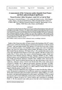
Figure 9: Measured threshold luminance as function of grating contrast.
ER -1
3.5
0.01 0.02 0.05 0.1 Contrast ǻL of Gabor Grating (in log 10 cd/m 2)
TK
0
300 400 500 Stimulus duration (in ms)
Repeats (200 ms)
Figure 8: a. Luminance thresholds as function of stimulus duration. b. Repeatability. The average lower threshold is 0.32 cd/m2 (σ = 0.09 cd/m2 ), while the upper threshold is 1716.3 cd/m2 (σ = 427.0 cd/m2 ). Thus, under the given experimental conditions, the simultaneous dynamic range of human vision is 3.73 log cd/m2 (σ = 0.18 log cd/m2 ), which is indicated in Figure 7. A one-way ANOVA was carried out to determine if there exist significant differences between the thresholds measured for each participant. We found that for both light and dark stimuli such differences do exist (dark: F(22, 230) = 36.49, p = 0.000, light: F(22, 230) = 20.62, p = 0.000); The standard deviations suggest that the inter-observer variability is low, meaning that the experiment has produced a reliable result. It also means that differences between individuals are small enough that these results can serve as guidance towards the design of high dynamic range display devices. Both authors repeated the experiment twice, results of which are shown in Figure 8b. As expected the standard deviations recorded in this manner are even lower than the inter-observer variability. TK’s thresholds are 0.477 cd/m2 (σ = 0.108) and 1520.2 cd/m2 (σ = 90.7), while ER’s thresholds are 0.423 cd/m2 (σ = 0.009) and 1818.6 cd/m2 (σ = 157.6). The standard deviations show a high degree of repeatability, which has prompted us to run subsequent experiments on the authors only.
5
Threshold (in log10 cd/m2)
Threshold (in log10 cd/m2)
Max. Display Luminance
Experiment 2: Stimulus Duration
There are several free parameters in the design of our experiment. To assess how they influence the perceived dynamic range, we have carried out further experiments, using the authors as participants. In Experiment 2, we identify the relation between stimulus duration and simultaneous dynamic range. We include stimulus display times from 100 ms to 500 ms in 100 ms intervals, as shown in Figure 8a. Shorter durations are not desirable, as it takes at least 90 ms for a stimulus to become detectable [Valeton and van Norren 1983]. As shown in Figure 8a, ER reached the maximum display luminance for 300, 400 and 500 ms., while this happened to TK for the 500 ms trials. Moreover, for the 500 ms. trials, TK reached the lower bound of the display range. While this limits our ability to infer a relationship between stimulus duration and luminance
threshold, there is a clear trend towards a higher simultaneous dynamic range for longer stimuli. The ease with which the limits of the display are reached in this experiment suggests that the ideal dynamic range of a monitor should be higher than the 4.7 log units that our prototype affords. In these experiments, the display is the only illuminant in the room. In practical scenarios however, the room will be illuminated, which will change the state of adaptation of the observer. It will also reduce contrast of the display, as it will reflect a portion of the incident light [Devlin et al. 2006] while scattering inside the display panel will further reduce contrast [Flynn and Badano 1999]. We expect that under such conditions the dynamic range required to accommodate the HVS’s will be higher.
6
Experiment 3: Contrast Magnitude
A second free parameter in our design is the amplitude A of the Gabor grating. We varied the grating amplitude from 0.01 to 0.1 log cd/m2 . However, this increases the risk of stimuli exceeding the display range. To prevent this, we lowered the adapting luminance for experiments 3 and 4 to 3 cd/m2 , and increased the presentation of the blank stimulus from 200 ms to 350 ms. In this configuration we are able to measure the upper threshold only. However, we surmise that the lower threshold would exhibit similar behavior. Nonetheless, the 2AFC is still interleaved with dark stimuli to maintain the observer’s state of full adaptation. However, no key presses needed to be given for the dark stimuli. Measuring only the upper threshold also enables the use of a grating amplitude of 0.01 log cd/m2 which would be too small for dark stimuli. The results for participants TK and ER are shown in Figure 9. The smallest of the amplitudes proved to yield a much more difficult task than any of the other amplitudes, as evidenced by the large standard deviations, and the large difference between the two participants. As expected, the remaining data points show good agreement between the participants, and have much lower variance, revealing that the upper threshold increases with increasing grating amplitude. Unfortunately with the current hardware we cannot test larger amplitudes without lowering the adapting luminance into the mesopic range, and thereby unduly complicating the analysis.
7
Experiment 4: Adapting Luminance
The final study examines the effect of changing the adapting luminance La , which we varied between 1.78 cd/m2 and 17.8 cd/m2 , i.e. between 0.25 and 1.25 in log units. We expect the upper threshold to co-vary to a large extent with the adapting luminance, given that previous studies have shown that adjusting La has the effect
Threshold (in log10 cd/m2)
3.5
ER TK
3.0
2.5
0.25
0.50
0.75 1.00 1.25 Adapting Luminance La (in log10 cd/m2)
Figure 10: The threshold luminance as function of adapting luminance La for participants TK and ER. of shifting the sigmoidal response function of the photoreceptors, without appreciably changing its shape. Thus, if the semi-saturation constant σ of Equation 1 and the adapting luminance La are equivalent, plotting the threshold luminance against the corresponding adapting luminance should result in a straight line with a slope of 1. For TK and ER varying La results in the thresholds shown in Figure 10. Note that the relationship between threshold luminance and adapting luminance is indeed a straight line in this plot. However, rather than being 1 the slope is 0.33. As can be seen in Figure 2, the relationship between adapting luminance La and semi-saturation constant σ is more complicated, which would explain our results. La0.33 ,
Thus, if we set σ = we find that the relationship between σ and the threshold luminance exhibits the anticipated behavior. This is consistent with the measurements of others for background luminances in the range that are examined here [Valeton and van Norren 1983; Normann and Perlman 1979].
8
Discussion
The development of high dynamic range display devices involves design decisions that are currently difficult to make without further knowledge of the HVS. In particular, the simultaneous dynamic range of human vision is an important design parameter, as it would be advantageous for HDR displays to exceed this range by a certain amount. However, the current literature is unclear about what the simultaneous dynamic range of human vision is. It is possible to infer the photoreceptor response curve from neurophysiological measurements, but this does not directly address the question of dynamic range. To resolve this issue, we have mounted a set of tightly controlled psychophysical experiments. With the aid of a high dynamic range display device we have established that under specific conditions the HVS functions over a range of 3.7 log units. Furthermore, we have determined the relationship between this range and several design parameters, including the contrast of the stimulus, the duration over which the stimulus is displayed, and the background luminance. We have found that the HVS is able to distinguish higher contrasts over a greater range of luminances, so that dependent on the application, a good HDR display should exceed 3.7 log units. However, within the limits of our current display, we are not able to assess by how much. The same holds for stimulus duration. If the stimulus can be inspected for longer, contrasts become visible more readily. Finally, the upper threshold relates to the adapting luminance in a
predictable manner. This means that if the HVS is adapted to higher luminances, the upper threshold will be elevated. Thus, if the display is located in a lit environment its maximum display luminance should also be increased. In all, this means that for HDR display devices to cover the full simultaneous dynamic range, their maximum display luminance should be increased with respect to current prototypes. The maximum display luminance of our display is rated at 3548 cd/m2 after calibration. For an adapting luminance that is near the boundary between photopic and mesopic vision, it is straightforward to create stimuli at the maximum display luminance that can still be distinguished. Our results therefore indicate that current display technologies do not yet adequately match the human visual capabilities. However, our experimental design has proven to be stable, which means that it would be possible for manufacturers to build a prototype display with a higher dynamic range and repeat these experiments with a small number of participants, extending the plots presented in this paper.
Acknowledgments We would like to thank Gerwin Damberg for suggesting this research, and for his thoughts and comments. Timo Kunkel’s research was sponsored by Dolby Canada.
References AGUILAR , M., AND S TILES , W. 1954. Saturation of the rod mechanism of the retina at high levels of stimulation. Journal of Modern Optics 1, 1, 59–65. ¨ , A. O., F LEMING , R., R IECKE , B., AND B ULTHOFF ¨ A KY UZ , H. H. 2007. Do HDR displays support LDR content? A psychophysical evaluation. ACM Transactions on Graphics 26, 3, 38. BADANO , A., AND F LYNN , M. J. 2000. Method for measuring veiling glare in high-performance display devices. Applied Optics 39, 13, 2059–2066. BAYLOR , D. A., H ODGKIN , A. L., AND L AMB , T. D. 1974. The electrical responses of turtle cones to flashes and steps of light. Journal of Physiology 242, 685–727. BAYLOR , D. A., N UNN , B. S., AND S CHNAPF, S. L. 1984. The photocurrent, noise and spectral sensitivity of rods of the monkey Macaca fascicularis. Journal of Physiology 357, 575–607. BAYLOR , D. A., N UNN , B. S., AND S CHNAPF, J. L. 1987. Spectral sensitivity of cones of the monkey Macaca fascicularis. Journal of Physiology 390, 145–160. B RAINARD , D. H. 1997. The psychophysics toolbox. Spatial Vision 10, 443–446. C RAWFORD , B. H. 1947. Visual adaptation in relation to brief conditioning stimuli. Proceedings of the Royal Society of London 128, 283–302. DAUGMAN , J. G. 1985. Unvertainty relations for resolution in space, spatial frequency, and orientation optimised by twodimensional visual cortical filters. Journal of the Optical Society of America A 2, 7, 1160–1169. DAVSON , H. 1990. Physiology of the Eye, 5th ed. Pergamon Press.
D EVLIN , K., C HALMERS , A., AND R EINHARD , E. 2006. Visual calibration and correction for ambient illumination. ACM Transactions on Applied Perception 3, 4, 429–452.
M OON , P., AND S PENCER , D. E. 1944. On the stiles-crawford effect. Journal of the Optical Society of America 34, 6, 319– 329.
FAIRCHILD , M. D., AND R ENIFF , L. 1995. Time course of chromatic adaptation for color-appearance judgments. Journal of the Optical Society of America A 12, 5, 824–832.
M YERS , R. L. 2002. Display Interfaces: Fundamentals and Standards. Wiley Series in Display Technology. Wiley Blackwell.
FAIRCHILD , M. D. 2005. Color Appearance Models, 2nd ed. Wiley-IS&T Series in Imaging Science and Technology. F ERWERDA , J. A., PATTANAIK , S. N., S HIRLEY, P., AND G REENBERG , D. P. 1996. A model of visual adaptation for realistic image synthesis. In Proceedings of the 23rd Annual Conference on Computer Graphics and Interactive Techniques, ACM, New York, 249–258. F ERWERDA , J. A. 2001. Elements of early vision for computer graphics. IEEE Computer Graphics and Applications 21, 5, 22– 33. F IELD , D. J. 1987. Relations between the statistics of natural images and the response properties of cortical cells. Journal of the Optical Society of America A 4, 12, 2379–2394. F LYNN , M. J., AND BADANO , A. 1999. Image quality degradation by light scattering in display devices. Journal of Digital Imaging 12, 2, 50–59. F UORTES , M. G. F., G UNKEL , R. D., AND RUSHTON , W. A. H. 1961. Increment thresholds in a subject deficient in cone vision. Journal of Physiology 156, 1, 179–192. G ABOR , D. 1946. Theory of communication. Journal of the Institute of Electrical Engineers 93, 3, 429–457. G ESCHEIDER , G. A. 1997. Psychophysics: The Fundamentals. Lawrence Erlbaum Associates. G ROOT , S. G., AND G EBHARD , J. W. 1952. Pupil size as determined by adapting luminance. Journal of the Optical Society of America 42, 7, 492–495.
DE
H ATEREN , H. 2005. A cellular and molecular model of response kinetics and adaptation in primate cones and horizontal cells. Journal of Vision 5, 4, 331–347.
VAN
H OOD , D. C., AND F INKELSTEIN , M. A. 1986. Visual sensitivity. In Handbook of Perception and Human Performance, K. Boff, L. Kaufman, and J. Thomas, Eds., vol. 1. Wiley, New York, 5–1 — 5–66. L EVITT, H. 1971. Transformed up-down methods in psychoacoustics. Journal of the Acoustical Society of America 49, 2, 467–477. ¨ M ACH , E. 1861. Uber das Sehen von Lagen und Winkeln durch die Bewegung des Auges. Sitzungsberichte der Kaiserlichen Akademie der Wissenschaften 43, 2, 215–224. M ANTIUK , R., R EMPEL , A. G., AND H EIDRICH , W. 2009. Display considerations for night and low-illumination viewing. In Proceedings of the 6th Symposium on Applied Perception in Graphics and Visualization, ACM, 53–58. M C M AHON , M. J., AND M AC L EOD , D. I. A. 2003. The origin of the oblique effect examined with pattern adaptation and masking. Journal of Vision 3, 3, 230–239. M ICHAELIS , L., AND M ENTEN , M. L. 1913. Die Kinetik der Invertinwerkung. Biochemische Zeitschrift 49.
NAKA , K. I., AND RUSHTON , W. A. H. 1966. S-potentials from luminosity units in the retina of fish (Cyprinidae). Journal of Physiology 185, 587–599. N ES , F. L., AND B OUMAN , M. A. 1967. Spatial modulation transfer in the human eye. Journal of the Optical Society of America 57, 3, 401–406.
VAN
N ORMANN , R. A., AND P ERLMAN , I. 1979. The effects of background illumination on the photoresponses of red and green cones. Journal of Physiology 286, 1, 491–507. P ELLI , D. G. 1997. The VideoToolbox software for visual psychophysics: Transforming numbers into movies. Spatial Vision 10, 437–442. P URVES , D., AND L OTTO , R. B. 2003. Why We See What We Do: An Empirical Theory of Vision. Sinauer Associates, Inc. R EMPEL , A. G., H EIDRICH , W., L I , H., AND M ANTIUK , R. 2009. Video viewing preferences for HDR displays under varying ambient illumination. In Proceedings of the 6th Symposium on Applied Perception in Graphics and Visualization, ACM, 45– 52. S EETZEN , H., W HITEHEAD , L. A., AND WARD , G. 2003. A high dynamic range display using low and high resolution modulators. The Society for Information Display International Symposium 34, 1, 1450–1453. S EETZEN , H., H EIDRICH , W., S TUERZLINGER , W., WARD , G., W HITEHEAD , L., T RENTACOSTE , M., G HOSH , A., AND VOROZCOVS , A. 2004. High dynamic range display systems. ACM Transactions on Graphics 23, 3, 760–768. S EETZEN , H., L I , H., Y E , L., H EIDRICH , W., W HITEHEAD , L., AND WARD , G. 2006. Observations of luminance, contrast and amplitude resolution of displays. Proceedings of the Society for Information Display 37, 1, 1229–1233. S PENCER , G., S HIRLEY, P., Z IMMERMAN , K., AND G REEN BERG , D. P. 1995. Physically-based glare effects for digital images. In SIGGRAPH ’95: Proceedings of the 22nd annual conference on Computer graphics and interactive techniques, ACM, 325–334. VALETON , J. M., AND VAN N ORREN , D. 1983. Light adaptation of primate cones: an analysis based on extracellular data. Vision Research 23, 12, 1539–1547. WALRAVEN , J., E NROTH -C UGELL , C., H OOD , D. C., M AC L EOD , D. I. A., AND S CHNAPF, J. L. 1990. The control of visual sensitivity. In Visual Perception: The Neurophysiological Foundations, L. Spillmann and J. S. Werner, Eds. Academic Press, Inc., San Diego, 53–102. WATSON , A., BARLOW, H., AND ROBSON , J. 1983. What does the eye see best? Nature 302, 5907, 419–421.