A recursive spatial equilibrium model for planning large-scale urban ...

Environment and Planning B: Planning and Design 2013, volume 40, pages 1027 – 1050

doi:10.1068/b39134

A recursive spatial equilibrium model for planning large-scale urban change Ying Jin, Marcial Echenique, Anthony Hargreaves Martin Centre for Architectural and Urban Studies, Department of Architecture, University of Cambridge, 1–5 Scroope Terrace, Cambridge CB2 1PX, England; e‑mail: [email protected]; [email protected]; [email protected] Received 3 August 2012; in revised form 25 April 2013; published online 19 October 2013 Abstract. This paper presents a recursive spatial equilibrium model for urban activity location and travel choices in large city regions that anticipate major development or restructuring. In the model, producer and consumer choices that adjust quickly to stimuli reach temporary equilibria subject to recursively updated activity churn, background trends, estate development, and transport supply. The city region’s performance at each time horizon affects the recursive variables for the next. The model builds on field leaders of urban general equilibrium, spatial interaction, and nonequilibrium dynamic models, and offers theoretical and practical improvements in order to fill an important gap in longrange urban forecasting. Linking the equilibrium and nonequilibrium models enables the simulation of path dependence in urban evolution trajectories that neither could produce in isolation. At the same time the model provides quantification of impacts of different policy interventions on a consistent basis for a given time horizon. The model is tested on the main archetypal urban development strategies for large-scale development and restructuring. Keywords: land-use and transport model, infrastructure investment, travel demand forecasting, spatial equilibrium, recursive dynamics, urban restructuring, urban futures

1 Introduction The 21st century as an ‘urban century’ has started to witness urban development and restructuring that are unprecedented in nature and scale. Over the next thirty to forty years accelerated urbanisation and lifestyle changes in the emerging economies are expected to lead to city building of a magnitude hitherto unseen in human history (UN Habitat, 2008); in countries that are already urbanised, some cities are still growing strongly. Numerous existing cities face challenges of restructuring and retrofit to tackle productivity growth, urban poverty, energy inefficiency, high per capita resource use, environmental degradation, and aging of citizens (Batty, 2010; Wegener, 1982; 2011). Bolder interventions have been called for (Fiorello et al, 2006; Wegener, 2011). Large-scale urban change may result from major new growth or restructuring. Evolution in the governance of cities has cast a new light upon growth and restructuring. In addition to existing powers of land-use planning and regulation, municipal governments are often offered responsibilities for infrastructure investment, major transport and urban service operations, and ultimately attracting inward investment. For instance, such powers have been gradually decentralised to the municipal level in China since the 1980s (Lin and Liu, 2000); the on‑going implementation of the 2010 election pledge (The Conservative Party, 2010) in the UK is a prominent example among the developed countries. Since the 2008 financial crisis, productivity growth has jumped to the top of the policy agenda across the world’s municipalities. Under tight public finance, productivity growth

1028

Y Jin, M Echenique, A Hargreaves

holds the key to social and environmental policies since the large investments required ultimately have to come from increased per capita output. This modifies the context for computer modelling that supports municipal decision making. It is instructive to review the experience in London, a UK city which has over the years seen a fair share of active development and use of computer models for major policy decisions on both new development and restructuring. 1.1 Policy concerns versus unmet modelling needs

In any city the most relevant policy concern is the viability to fund (electoral) commitments to local constituencies. This was true even before the financial crisis. Volterra and CBP (2007, page 47) provide an insight into the unmet modelling needs in London, particularly concerning “the links between productivity, wages and rents and the full implications of these for output growth”. They go on to list the unanswered questions as: What are the behavioural responses to overcrowding and to new transport availability? What are the effects of co-location and clustering of different firms, and do these vary among industries? What are the trade patterns and how do they change? How can we test that the models we use reflect the world in which we operate? Decentralised decision making strengthens the above concerns. Local authorities are focused on the ‘business case’ of any intervention and feasibility under financial and fiscal constraints. Since any assessment of a large development proposal will be subject to debate, the models must be transparent and empirically robust (Rosewell, 2011). The criticism is that methods for assessment (eg, of transport investments in the UK) are “unconnected to the real economy” (Wenban-Smith, 2011). Similarly unmet policy needs are apparent across the OECD (OECD, 2012). In the developing countries our experience shows that the policy concerns are similar, but the modelling tools remain unavailable in most cities. It seems that it was not technical complexity of models per se that deterred policy applications. For instance, the aspiration for identifying ‘the full implications’ of productivity, wages, and rents shows that there is a genuine appetite for general equilibrium modelling. However, large urban models are seen as ‘black boxes’ by critics (Lee, 1973) as well as modellers (Eliasson and Mattsson, 2001), and users often avoid the large models, even if that means reduced form rather than general equilibrium modelling (DfT, 2006; Volterra and CBP, 2007). Short mayoral election cycles and the need to face the public call for quick turnaround and transparency. The world after the financial crisis does not seem to have fundamentally altered the key modelling questions. Rather, the need to understand drivers to productivity and offer practical insights to policy making are highlighted. This means that the models need to operate in the world of markets, prices, finance, budget constraints, physical and institutional inertia, individual behaviour, and their combined impacts. 1.2 Existing modelling methods

It is useful to contrast user needs with what is already available for policy modelling. Such models sprang from many different fields and disciplines, and they are far from paradigm convergence (Batty, 2009). Given the traditional emphasis on land-use and transport planning, the main urban models in policy use since Lowry (1964) are built on spatial interaction models (Batty, 1976; Wilson, 1967). Effective and practical models have been created for assessing property development and transport options at detailed geographic scales through a close integration of the spatial interaction model with random utility theory (McFadden, 1974), national/regional input– output tables (Leontief, 1986), land-use and floorspace stock market models (Echenique, 2004; Echenique et al, 1969), transport demand forecasting (Ben-Akiva and Lerman, 1985; Daly and Zachary, 1978; Domencich and McFadden, 1975), road traffic assignment

RES model for planning large-scale urban change

1029

(Sheffi, 1985), GIS and big data analyses (Batty, 2010; Batty et al, 2013). Their strengths lie in the explicit incorporation of planning and infrastructure constraints and the incorporation of policy inputs over explicit time horizons. However, those models rarely address endogenous productivity growth or urban dynamics. A second strand of models investigates general equilibrium of the spatial economy. The relationships between the economy, activity location, and transport costs have been a focus of new economic geography (Fujita, 1989; Fujita et al, 1999; Krugman, 1991; Venables, 1996) and of spatial general equilibrium models (Anas and Kim, 1996; Anas and Liu, 2007; Bröcker, 1998; Ivanova and Tavasszy, 2007; Oosterhaven et al, 2001). Those models are focused on the effects of spatial costs on producers and consumers whilst giving a fuller representation of product varieties and economies of scale. Some models account for urban agglomeration and related productivity effects. Significant progress has been made in empirical model estimation (Redding, 2010). Production, trade, transport demand, and location are endogenously and mutually determined at spatial general equilibrium. Although, like the spatial interaction models, they can be used for discrete time horizons, existing spatial equilibrium models in their published form tend to focus on the end state rather than on the trajectories leading to the equilibrated state. Anas and Liu (2007) have introduced a dynamic property development sector within a general equilibrium model with exogenously determined total size of the city and of development. Dynamic general equilibrium models that represent intergeneration linkages and forward-looking behaviour have been at an exploratory stage (see Bröcker and Korzhenevych, 2011) or on the longer term research agenda (Anas, 2013). A third strand of models is focused on urban dynamics, which are either represented in the aggregate (Allen, 1997; Forrester, 1969; Simmonds, 2001; Wegener, 2001; Wilson, 2000; Zondag and de Jong, 2011) or at a microlevel through cellular automata, agent-based models, and other forms of microsimulation (Batty, 2005; Chapin and Weiss, 1968; Clarke, 1996; Ingram et al, 1972). Microlevel dynamic models have been developed for land-use activities (UrbanSim, 2011; Waddell, 2002) and traffic flows (Nagel et al, 1999). They offer insights into microscopic interactions among agents, particularly in property development and traffic management. They also introduce physical inertia explicitly. However, they are predominantly used for investigating mechanisms and system-level emergence of microscopic interactions rather than for policy analysis (Batty, 2009), with a few exceptions such as those models developed by Wegener (2001), Simmonds (2001), Zondag and de Jong (2011), and UrbanSim (2011) which have been used for policy studies. A prominent feature of the applied models is their disregard for market equilibrium (Simmonds et al, 2013). It is clear that the needs of policy analysis will be better served if the model features could be applied across paradigms.(1) In particular, policy making requires not only insights into interdependencies at any point in time but also into how cities evolve. In summary, cities facing major growth and restructuring would require planning models that can examine (1) implications of planned intervention on productivity, wages, and rents over policy horizons that relate to tenure lengths of mayoral offices; (2) effects of planning, building, and infrastructure constraints which are dominated by inertia and take decades to reach any equilibrated state if ever; and (3) dynamics of people and investment in response to prices, productivity, and citizens’ well-being. In addition, such models should (4) be built upon technical data that most cities already have, such as censuses, input–output tables, urban traffic models, travel behaviour surveys, and any emerging big data. So far as we are aware, (1)

Where such progress has been made, the results are promising: for example, in linking spatial interaction and general equilibrium modelling (de la Barra, 1989; Echenique, 2004), cellular automata with input–output modelling (eg, White et al, 2000), or incorporating principles of microsimulation within aggregate urban land-use activity and stock modelling (Simmonds et al, 2013; Wegener, 2001).

1030


no models currently meet the above four requirements simultaneously, least of all in those emerging economies that matter the most to world poverty alleviation and sustainability. 1.3 Aims of this paper

The aims of this paper are (1) to present the design of a new, generic model that starts to incorporate the above four requirements simultaneously for practical urban applications; and (2) to test it on a wide range of archetypal development scenarios for insights into fundamental model assumptions, roles of key parameters, and the added value of the new method. The tests help to set a prioritised research agenda for empirical implementation for assessing individual projects and policy initiatives. The paper provides a summary of the model and tests for model users whilst addressing the key concerns of specialist modellers. More specialist material on equations, data, algorithm, and tests are presented in a supplementary working paper (Jin et al, 2013). 2 Model design We consider each model component in turn before linking them together. Key concepts are reviewed where the context requires but space does not allow a literature survey—for such surveys see Wegener (2005; 2011), Hunt et al (2005), Iacono et al (2008), and Batty (2009). As it is a spatial model, locations are defined as discrete and contiguous zones; the model divides the world into two categories of zones: ‘internal’ ones that represent areas within a city region;(2) and ‘external’ ones for the city region to trade with and to exchange migrants, supercommuters, and investment funds with. 2.1 Components for a new model

We follow a widely shared convention between spatial interaction and general equilibrium models and classify the economy into producers which include private, public, and voluntary businesses; and final consumers which include households, governments, collectives, investors, and exports. We further follow that convention and consider trade in labour, goods, and services between locations which is determined simultaneously with prices at market equilibrium, subject to idiosyncratic circumstances. We follow nonequilibrium dynamic models and define the stock of existing urban activities, buildings, transport infrastructure, and land as stock constraints which may be updated periodically subject to background trends, inertia, investment, and planning regulations. Finally, we consider how boundary conditions—such as business relocation and household migration between internal and external areas and cross-boundary investment—occur subject to prices, physical constraints, citizens’ well-being, and idiosyncratic circumstances. For simplicity, when the model components are discussed for one period only the time period subscripts t, t + 1, etc, are omitted; to account for flows of money (eg, production, consumption) and effort (eg, hours of labour, utility gains) all such quantities are defined in annual units unless noted otherwise. 2.1.1 Producers The producers are represented by a set of production functions that define how they use capital, labour, properties, raw materials, and services, particularly how their input choices and productivity change with prices and externalities. A nested Cobb–Douglas–constant elasticity of substitution (CD‑CES) function has been broadly accepted as a standard for this purpose in spatial general equilibrium analyses since Krugman (1991) and Fujita et al (1999). We follow Anas and Liu (2007), who developed a leading urban general equilibrium model, and define

(2)

This is usually a reasonably self-contained area for daily commutes.


1031

the production function as a variant of their CD-CES specification: n j

n j

n vn j

dn wn i n i n j

/ (L

X = E A (K ) c n j

w

/ (B

) m c

nn kn g n g n j

k

) m

%(Y

mn c mn j

)

,

(1)

m

where  X nj  is the output of industry n in zone j. The main inputs to production are capital K, labour L, buildings B, and intermediate inputs Y; and the function implies constant internal returns to scale of production through specifying the sum of cost share parameters for the n respective input groups, v n + d + n n + m c mn = 1 . For w varieties of labour and k varieties of buildings, a CES function is used to represent the substitution effects within each input, the elasticities of substitution being governed by parameters i n  and  g n  . A nj  is a function of the economic mass for producer n in zone j that represents Hicksian-neutral total factor productivity effects resulting from learning and transfer of tacit knowledge (Graham and Kim, 2008; Rice et al, 2006), which are an important component of urban agglomeration effects. We define  A nj = A nj (M nj / M nj ) r, where  A nj  is a constant representing baseline economic mass effects;  M nj  is a function of the economic mass accessible by producer n from zone j;  M nj  is a constant representing the baseline economic mass for product n in zone j; and π is a parameter to be calibrated. Following Graham et al (2009) we define  M nj = w d n i Lwi (dij) - \ , where  M nj  is a measure of the accumulated economic mass for industry n in location j;  Lwi  is the total size of employment of type w that is relevant to industry n in zone i; dij  is the economic distance from location i to location j; and \> 0 is a distance-decay parameter. Finally, E nj  is a constant scalar representing any additional zonal effects on total factor productivity, which is to be calibrated empirically. The production function (1) differs from that of Anas and Liu (2007) in two ways. First, an economic mass function A nj  is introduced to represent increasing external return to scale in production: that is, those urban agglomeration effects that arise from land-use and transport changes.(3) Secondly, labour and intermediate inputs enter the production as quantities by zone rather than by zone pair. This makes it easier to calibrate the models empirically, because zonal observations are much more easily found; also the production function is more readily interfaced with existing social accounting matrices (Echenique et al, 2013) and fourstep transport models for commuting and for goods transport (see subsection 2.1.3). Each type of labour and of intermediate inputs consists of commuters and goods/services, respectively, supplied from all available model zones i (including i = j); the sourcing of those inputs among zones is modelled through spatial interaction. Each type of building stock in zone j is fixed for the period and updated in the following period as a result of obsolescence, renovation, new construction, etc represented in a recursive model (see subsection 2.1.4). We follow standard assumptions that producers are cost minimisers under budget and input supply constraints, and operate with zero economic rent and constant internal returns to scale. The price of goods or service n produced in zone j can then be derived as an average and marginal cost. In turn, given X nj , the demands for inputs of capital, labour, buildings, and intermediate inputs can be derived from equation (1).(4) Imports into the city region are included as external production.

/

/

(3)

/

When such agglomeration effects are strong the model could produce multiple equilibria (Anas and Kim, 1996). Here we expect the parameter π for most cities to be generally below 0.1 (Graham and Kim, 2008; Rice et al, 2006; Rosenthal and Strange, 2004). Zhu (2012) has tested parameter π in the range 0.0–0.2 for primary and secondary industries, and 0.0–0.4 for tertiary industries with a model calibrated for southern England and found that a single quilibrium exists from a reasonable range of alternative input values. The higher the π value, the more is required in calibration to check for possible multiple equilibria. (4) For further equations and discussions, see Jin et al (2013). This split between summary and detail also applies to the rest of this paper.

1032


2.1.2 Final consumers For the final consumers, we model household choices and leave government budgets, other collective spending, investment decisions, and exports as scenario inputs. The reconciliation between production output (subsection 2.1.1), budget, spending, and investment is a policy decision that should be made explicit as model input. On the other hand, inward investment and export levels may be recursively updated to reflect productivity and prices in the city region. Household choices here refer to how households source goods and services, choose where to live, and, in the case of working households, determine how to divide time between work and leisure on the basis of utility, prices, and externalities. Households are assumed to maximise utility under constraints of income and time. We follow Anas and Rhee (2006) in including households’ consumption of leisure time as well as goods, services, and housing: V iH =

/ ^a

mH

m

ln zimH h + b H ln ;

/ (b k

1 H kH g g H i

) E

+ c H ln liH ,

(2)

where ViH  defines the economic well-being for household type H which is derived from consumption and leisure in residential zone i;  zimH  is the demand per household H for goods/ services of type m in zone i; similarly bikH  is the housing demand; liH  is the leisure time in hours for household of type H during working days of the year; a mH , b H , and c H ,  where  ` m a mH j + b H + c H = 1 , are parameters for consumption in goods/services, housing, and leisure time, respectively; and g H  is a parameter for the nested CES function for choosing among housing varieties. Household consumption utility increases not only through consumption, but also through a rise in the number of varieties of housing available for better matching with needs. Households may also trade off consumption against leisure time. Households’ demands for consumption and leisure time are derived through the household budget and the level of incomes, prices, and rents. The households may be segmented by socioeconomic profile, life-cycle, size, etc,

/

2.1.3 Location choices and trade patterns In many cities, commuting, shopping, and goods delivery patterns and residential location choice have already been modelled by spatial interaction models that are embedded in transport models, often with a richness in market segmentation and behavioural calibration that is worth building upon. The zonal production and consumption functions defined above facilitate a relatively easy interface with spatial interaction models. Following the random utility interpretation of such models (McFadden, 1974), if the location utility for obtaining input m in zone i for user n in zone j is oijm = oim - dijm - }ijm - Wim + f m  (where  oim  is the utility of input m from zone i; dijm  is a generalised transport cost function including travel and logistical costs to transport a unit of input m from zone i to zone j;  }ijm  and  Wim  are observable nonmonetary barriers for trading from zone i to zone j and for production in zone i, respectively; and  fijm  is a constant representing unobservable idiosyncratic variations in utility that follow an independent and identical distribution of the Gumbel type) then the trade volume  Zijm  can be expressed generally as: Zijm = Z mj *

Sim exp 6 m m (oim - dijm - }ijm - Wim)@ , Sim exp 6 m m (oim - dijm - }ijm - Wim)@ 4

/ i

(3)

m where  Z mn j  is the total demand for input m by user n in zone j; S i  is a size term that corrects for the bias introduced by the uneven sizes of zones in the model (see Ben-Akiva and Lerman, 1985); and  m m  is a scale parameter that measures the concentration of trade among alternative sources which is empirically calibrated along with parameters  }ijm  and  Wim .


1033

More specifically, for sourcing of goods and services, oim =- pim , where  pim  is the factorygate price for goods m(5). This applies to both intermediate and consumer goods/services, including the special cases where the services are travel for leisure and personal business. Commuter households choose where to live based on oim = ViH and on dijm  , a generalised cost function for commuting. For noncommuter households, equation (3) is relevant only in cases where their residential locations are determined by previous commuting choices. An important aspect of spatial choice that has been overlooked in both urban general equilibrium models and land-use and transport interaction models at the city-region scale is the formulation of the dijm  function. City regions with a reasonably self-contained commuting catchment today tend to have a radius of 50 km or more. At this metropolitan scale, extensive analyses of travel choices data show that a dijm  function that is linear to travel costs and times will have great difficulties in representing realistic demand elasticities throughout; a nonlinear, Box–Cox transformation of utilities is required (Gaudry and Laferrière, 1989). Fox et al (2009) put forward a log-linear transformation that is a close equivalent to the Box– Cox function whilst being easier to calibrate. This function should fit, in the form:

/h

dijmn = a m a

k

mn k

/h

m m \ijk k + (1 - a ) ln a

k

mn k

m m \ijk k - a ,

(4)

mn  are the attributes of travel, such as cost or time, and the h kmn  and a m  are where the \ijk parameters.

2.1.4 Stock constraints We define stock constraints in line with Wegener (2001) to cover not only land, buildings, and transport infrastructure but also existing urban activities such as job and home locations which may evolve or ‘churn’ slowly. For instance, there may be a lag of many years between a utility change and household relocation. For each period, only a proportion of the existing households will be ready to move. Whilst the commuter households make their choices according to equation (3), the moving noncommuter households face the utility level U Hj = V jH - W Hj - h H dijH + f Hj , where W Hj  is a nonmonetary barrier for locating in zone j, and dijH  is a measure of perceived distance from zone i to zone j. We thus obtain a discrete choice model: X lijH = X liH *

S Hj exp 6 m H (V jH - W Hj - dijH )@ . S Hj exp 6 m H (V jH - W Hj - dijH )@ 4

/

(5)

j

At spatial equilibrium, the demand for all types of buildings stock, Bik  and bik , must be equal to available supply, B| kj  and b| kj .  B| kj  and b| kj  , as well as the associated land supply, respond to demand through development/restructuring but subject to regulation, planning, speculation, procurement, construction/renovation, commission and decommission, and inertia. It is thus more appropriate for a model user to specify detailed estate development plans, subject to expected rental revenue and costs. The model can then account for the asymmetry between growth and decline—for example, in the case of business buildings: (6) B| kj (t + 1) = ^1 - Y kj h B| kj (t) + Bv kj (t + 1), if B kj (t + 1) H B kj (t) , B| kj (+ 1) = _1 - Y kj i B| kj (t),

(5)

otherwise.

(7)

Here we present a simplified model by assuming that input m is shipped straight from zone i to zone j. The logistical channels may be added through a supply-chains model consisting of a series of random utility models for intermediate logistical stages; for an application to the UK, see WSP UK Ltd (2005).

1034


In equation (6), as the total building demand for type k in zone j increases, the existing building stock is depleted by Y kj (0 G Y kj G 1)  through demolition and conversion, and the user-specified building stock increment at period t + 1, Bv kj (t + 1) , is added for period t + 1. In equation (7), as the total demand falls, the user-specified building increment does not materialise, and the existing building stock is depleted by Y kj (0 G Y kj G 1) . In other words, when building demand increases, the user-specified plan is adopted; if demand falls, the existing stock will reduce through depletion, and the user-specified plan is left unimplemented. Similar equations may apply to housing or urban land. The equations reflect the indivisibility of user’s development plans (ie, all or nothing for the new stock increment) and can be further refined as proposed by Glaeser and Gyourko (2005). Similarly, transport infrastructure and services respond to demand subject to regulation, planning, procurement, construction/renovation, commission and decommission, and thus respond to demand slowly and indivisibly. Like land and buildings, user-defined transport supply scenarios are likely to be the most appropriate subject to transport revenues and costs; the growth/decline asymmetry can be applied: that is, new projects are implemented only in the test if the related demand grows. 2.1.5 Boundary conditions External shocks cover decisions that at least partly depend upon factors outside the city region. Business investment and household migration across the city region boundary are such examples. Naturally, external shocks are case dependent. Traditionally external shocks are exogenous, scenario inputs. Nevertheless, policy makers are interested in how changes within a city region may trigger certain shocks under prevailing external conditions. For such decisions we continue to follow the notion of utility: UI = VI + f I , where VI  is the measurable average utility for the city region as a whole, and f I  is a Gumbel-distributed error term. This leads to a discrete choice model V(It

+ 1)

t + 1) ) = V(All

S I(t) 6 exp (m I‑ E V I(t))@ 3 , S I(t) 6 exp (m I‑ E V I(t))@ + S E(t) 6 exp (m I‑ E V E(t))@

(8)

where V I  predicts the activity (eg, migrants or investment) that chooses the city region, and SI  is a size term. All terms with an E subscript denote corresponding values assumed for the external area. Under this random utility framework which accounts for idiosyncratic circumstances through parameter m I - E , we may define a migration function V I(t) = V IM (t) = VrIH (t) - d IM-(tE) for migration choices subject to average household utility  VrIH  and migratory distance d IM- E  at period t, and a business floorspace investment function Vt(t) = V IB (t) = ln (Rr IB (t)) - ln (pr I(t)) + r ln (Mr I(t)) that consists of expected rentals Rr IB  , average production cost  pr I , and productivity effects from the economic mass  r ln (Mr I)  at period t. 2.2 Model assembly

Central to model assembly is the fact that urban change processes vary over time scales (Simmonds et al, 2013; Wegener et al, 1986). Some processes adapt quickly to constraints and are thus amenable to equilibrium modelling, such as producer and household relocation and transport choices; others are more inertia prone, lumpy, and indivisible, such as estate development, transport supply, and life-cycle churns of producers and households. Existing spatial interaction and general equilibrium models, to a varied extent, all adopt a strategy to solve for equilibrium quantities and prices subject to exogenous constraints; the equilibrium condition provides a consistent platform for comparing alternative policy interventions at each time horizon, but such models rely on exogenous scenarios to articulate trajectories between time horizons. Nonequilibrium dynamic models offer insights into the effects of life-cycles, churns, and inertia on temporal trajectories, but have to rely on an interface with other models with an equilibrium mechanism (most often a transport model)


1035

to assess any costs and benefits. Cities facing large urban change require both cross-sectional assessment of prices, rents, and wages and the cumulative effects of urban evolution. This calls for a more radical interface between equilibrium and nonequilibrium models. An appropriate articulation of the model components has to be considered for model calibration, validation, and forecasting. Calibration of a recursive model requires not only a representation of the city region at a base year t, but also at least one transitional period to the next horizon t + 1, preferably more. For calibration at base year t, all boundary conditions and constraints including the activity stocks are needed as inputs, as are the quantities and prices of goods and services, labour, buildings, land, and trade patterns. The model estimates the demand for goods and services, labour, buildings, land, travel, traffic flows, and all associated prices based on input boundary conditions, stock constraints, and an initial set of model parameters that are derived through successive partial equilibrium model estimations (see the left-half of figure 1). The solution algorithm proceeds iteratively through each of the markets until all demand and prices reach equilibrium. The model predictions are compared with known zonal quantities and prices to refine the parameters. The model parameters are then retained for use for period t + 1. For transition to period t + 1, the known changes in boundary conditions, stock constraints, and associated knowledge on policy interventions are used to establish recursive models that

Figure 1. Main information flows within and between recursive spatial equilibria.

1036


predict boundary conditions and stock constraints for period t + 1. The recursive models may include one-off events which enter as period-specific constants. The spatial equilibrium model is run in forecasting mode for period t + 1. The model predictions are validated through comparing with known zonal quantities and prices for period t + 1 which have not been used in model calibration. The recursive and spatial equilibrium model calibration may have to be repeated many times in a calibration–validation loop until a satisfactory goodness of fit has been achieved (see the right-hand half of figure 1). Ideally, more than one known transition period exists so that the recursive models for boundary conditions and stock constraints can be tested repeatedly, and the model builds up a validated track record. In practice, it is rarely feasible to trace back more than one historic period for data problems and modeller resources. An effective way to achieve multipleperiod validation may be to retain existing models and extend them through time, and use the successive model development exercises to extend the series of recursive models. From period t + n (n H 2) the model will be used in forecasting mode. The recursive and spatial equilibrium models share the same running procedure as for model validation at period t + 1. Whilst the spatial equilibrium model for each horizon t + n (n H 0) is a static equilibrium model, the recursive model representing the transition of boundary conditions and stock constraints are nonequilibrium in nature. Although the recursive models are perhaps the most uncertain to begin with, their outputs for transition between time horizons are nevertheless made plain to see by all model users. In fact, in the case of forecasting, the model users may wish to intervene and revise the projections, either at the city-region level or for specific zones, as a form of scenario design. Nevertheless, a gradual establishment of evidence-based recursive models is particularly useful for radical development and restructuring scenarios— however much they are interested in such scenarios, the far-sighted decision makers might not want to be seen specifying them for political reasons. The number of years elapsed between two modelled time horizons is a local matter. The standard assumption of the recursive model is that an urban administration goes through a stereotypical cycle from new initiatives to policy implementation and ultimately to the lame-duck phase: in such cases, the majority of the stimuli to boundary condition and stock constraint changes would occur early in the period; producers and consumers then adapt before the next round of radical changes. However, development cycles are hardly universal, and the time horizons are heavily constrained by data availability (eg, the census years) and masterplan horizons. Locally specific considerations are thus crucial in determining the period length. In our experience, ten or more years may be required for development and restructuring effects to work through producer and consumer choices. This is true even during the recent fast growth in China since the late 1970s, where distinct policy cycles are generally around ten years (Zhang, 2010). 2.3 Model outputs for policy assessment

The model outputs are quantities (production, factor inputs, and consumer demand) and prices (of goods/services, wages, and rents) in each zone, and movements of people and goods/ services between zones. A multimodal transport model or a collection of unimodal traffic models need to be incorporated to estimate travel demand, costs, operation characteristics, and congestion/overcrowding levels. The outputs provide the basis for assessing economic, social, and environmental benefits (Echenique et al, 2012). In the model, two types of prices are accounted for in parallel under spatial interaction: the consumption price of inputs that come from different zones are calculated as an average of the delivered prices weighted by respective trade volumes; the average utilities of the inputs are calculated as a log-sum (Ben-Akiva and Lerman, 1985; Williams, 1977) of the delivered prices.


1037

Household utility is not linear in income and the marginal utility of income varies between policies and among zone pairs of spatial interaction (Anas and Rhee, 2006). The overall consumer surplus, ΔC, in the city region as a household well-being measure may be defined as the change in average household utility divided by the average marginal utility of money: 1 1 1 TC = ^ V Alternative - V Base h : 2 a Alternative + Base kD , X X

(9)

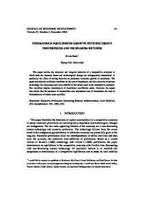
where V Base  and V Alternative  are the average household utilities, and X Base  and  X Alternative  are the average household incomes for the Base and Alternative scenarios, respectively. 3 Model tests Although the model components follow three well-established model traditions, the new model design still needs thorough in-lab testing. This is because, first, the interactions between the recursive and equilibrium components create many new mechanisms that do not exist in current models. Secondly, an understanding of the range and uncertainty of parameter values helps to develop a prioritised agenda for empirical model estimation. Thirdly, largescale urban change may be a challenge for the spatial equilibrium model to converge. We set up test model code in MatLab (The MathWorks Inc.) with a flexible zone dimension. When it is used for a one-zone model, all model results may be traced easily by hand. Here we use a model with twelve zones which retains the fundamental features of a city region and can represent archetypal urban development strategies, in order to pressuretest the model with easily manageable data tables. We present the key results here and further details are to be found in Jin et al (2013). We specify a narrow peninsular city region with the following zones: (1) an older, denser city centre at the cape where businesses concentrates with limited housing; (2) a built‑up inner city with both homes and jobs; (3) a contiguous outer urban area where housing dominates; (4) a greenbelt where development has been restricted; (5) a far suburb beyond the greenbelt with multiple commercial centres scattered among towns and villages; (6) a wider rural hinterland which is sparsely populated (figure 2). We further distinguish a freestanding city in the far suburb, and five small areas which are the main catchment of large rail stations—we code them as zones 10 and R1–R5 respectively. The spatial configuration of this model has made land-use patterns more explicit, but otherwise it follows the tradition of the ‘long narrow city’ of Solow and Vickrey (1971), applied, for example, by Anas and Kim (1996) and Eliasson and Mattsson (2001). To make the data flows easy to trace in a complex model, we make a number of simplifications. We assume that the total population in our city region is 1 million at time t (say 2010). There are nine other city regions of the same size in the country (thus the total number of households in the country is 10 million), although there are none nearby.(6) Periodically, households in other city regions as well as this one compare their well-being and make decisions to migrate between them. The city regions altogether face a population growth of 2.5 million per decade, thus doubling at period t + 4 (2050) to 20 million. The boundary conditions are migration subject to average household migration utilities V IL  and business floorspace investment subject to attractiveness function V IB  (see subsection 2.1.5). It is also subject to the reservation utility for the rest of the country, VE . The solving algorithm of the spatial equilibrium model is shown in figure 3. We define one type of household. Each household supplies one worker who fills one job. Trade across the city region boundary is zero; the workers produce a product that is entirely consumed by the households in the city region. The households also own the estate properties (6)

If there are, the internal modelled area shown in figure 2 may be expanded to include them.

1038


Centroid of a zone Point zone (rail hub) Coast line Zone boundary Road Road+metro Rail

Figure 2. The model area, transport links, and zone numbers. Diagram not to scale; physical dimensions are specified by land-use and transport data.

Figure 3. Model-solving algorithm.


1039

collectively and share out the rental income equally. We assume an average household wage income of around £12 000 (or US $18 000) per year.(7) There are two types of housing (houses and apartments) and two types of business floorspace (bespoke and generic). 3.1 Model parameterisation

We take parameter values from established models. Where there are no commonly accepted parameters we carry out sensitivity tests in the model and adopt value ranges by judgment. Table 1 lists the model parameters that have been specified in the equations. Table 1. Model parameters and their sources. Model parameter

Value(s)

Sources

d n (labour cost share) n n (business floorspace cost share) o n (capital cost share) c mn (intermediate inputs cost share) g n (business floorspace variety effects) E nj (residual total factor productivity multiplier) r (economic mass effects on productivity) a (household utility parameter for goods/ service) b (household utility parameter for housing) c H (household utility parameter for leisure time) g H (housing variety effects) m m (scale parameter for spatial interaction model)

0.86 0.14 0.00 0.00 0.90 1

Anas and Rhee (2006) Anas and Rhee (2006) Anas and Rhee (2006) Anas and Rhee (2006) Own sensitivity tests Anas and Rhee (2006)

0.05-0.10 0.36

DfT (2006); Graham and Kim (2008) Anas and Rhee (2006)

0.15

Anas and Rhee (2006)

0.49

Anas and Rhee (2006)

0.90 1

Own sensitivity tests Calibrated to reproduce an average commuting distance that is compatible with mid-income commuters in the London region in 1991 (Jin et al, 2002), in conjunction with a m  below The zones are featureless other than represented by land-use and transport data See above

}ijm, Wim, }ijH , W Hj (zone-specific attractiveness) a m (log–linear travel cost function parameter) h km (log–linear travel cost function parameter)

0 for all i, j 0.0005

Y kj (building stock depletion)

0

m IH E (scale parameter for household migration model) m IB E (scale parameter for business floorspace investment model) Total number of working days a year Hours per day Cost for delivering a unit of local service as percentage of commuting trip cost

1.0-4.0

A multiplier to converts travel costs and times of one trip to annual (2 trips a day, 250 days a year) Building stock depletion is not included here for simplicity Own sensitivity tests

1.0

Own sensitivity tests

250 24 10%

Anas and Rhee (2006) Anas and Rhee (2006) Anas and Rhee (2006)

(7)

500

This income is supplemented by shared rental income, implying an average household income of £21 000; this represents a reasonably affluent profile that the leading emerging economies are currently aiming towards.

1040


3.2 Model runs

Floorspace (m2)

We present three types of run to highlight the key features of the model: (1) the base year t which represents 2010; (2) a set of static equilibrium runs for period t + 4 (2050) with given boundary conditions; (3) a set of recursive equilibrium runs from 2010 to 2050.

1

2

3

4

5

6

all

10

1

2

3

4

5

6

all

10

Zone Zone (a) (b) Figure 4. Floorspace constraints by zone in year t (2010): (a) business, (b) housing.

13.8 Price (£/unit)

Million units

1200 800 400

(a)

0

13.4 13.2 13.0

(b)

200 Rent (£/m2)

1200 Rent (£/m2)

13.6

800 400

150 100 50 0

0

(d)

(c)

1200

400

(e) Wage (£/hour)

Thousands

800

0

6.3 6.2 6.1 6.0

400 0

1080 1040 1000

(h)

7.4

Utilities (utils)

Utilities (utils)

(g) 7.2 7.0 6.8

800

(f) Consumption (units)

Thousands

1200

1

2

3

4 5 Zone

6

10

all

2 1 0

1

2

3

4 5 Zone

6

10

all

(j) (i) Figure 5. Model output quantities and prices by zone, in year t (2010): (a) production output; (b) product prices; (c) business rents; (d) housing rents; (e) number of jobs; (f) number of households; (g) wages (home location); (h) consumption per household; (i) consumption utilities; (j) commuter location utilities.


1041

Distance (km)

50 40 30 20 10 0

Cost (pence)

150 100 50 0

Time (min)

3.2.1 Model run for t (2010) The model starts with inputs of transport supply, stock of housing and business buildings (figure 4), stock of households and jobs, and boundary condition (total households = 1 million) at time t (2010) for a static spatial equilibrium run. The output activity stock in this case equals the input; the model also outputs prices, rents, wages, and household utilities by zone (figure 5). Through the interface with the transport model, the travel distances, costs, and times incurred by labour and product flows are computed (which are summarised in figure 6). The model outputs depict a polycentric city region where the densely built-up areas have short average travel distances, long travel times, and high rents; the reverse is the case in the suburbs.

60 40 20 0

1

2

3

4

5 6 10 Zone

all

1

2

3

4

5 6 10 Zone

all

1

2

3

4

5 6 10 Zone

all

(c) (b) Figure 6. Model output average trip distances, travel costs, and travel times by purpose by zone, in year t (2010) for: (a) commuting—by home origin; (b) commuting—by workplace; (c) goods and services—by household location. (a)

3.2.2 Static spatial equilibria for 2050 Before running the model recursively, we tested the spatial equilibrium component by static runs for four archetypal scenarios: (1) trend growth which targets development opportunities through inner-city regeneration and greenfield development beyond the greenbelt, (2)  compact development of existing built-up areas without new greenfield land supply, (3) expansion of garden suburbs outside built-up areas at prevailing suburban densities, and (4) densification around urban rail hub locations which is an upscaled version of transit-oriented development. For these static runs we assume that the city region will grow at the country-average rate: that is, doubling the number of households to 2 million in 2050. Half of the expected floorspace construction will be natural growth which occurs pro rata to existing zonal stock, and the remainder is specified by the respective planning scenarios. For each scenario (2)–(4), three variants are tested: (a) maintaining the status quo: average floorspace per household and per job, and average travel costs and times remain unchanged from 2010;(8) (b) scale of floorspace construction following zonal profiles per household and per job under each planning scenario: 30% less per household and per job in dense built‑up zones and 30% more in suburban and rural zones; (c) accompanying traffic speeds following zonal profiles in addition to zonal floorspace profiles: in the case of compact development and garden suburbs, traffic congestion worsens—average intrazonal travel times increase by 5 minutes, and the access times to and from those zones increase by 10 minutes per trip; in (8)

This follows pragmatic policy targets used in many cities where infrastructure investment aims to keep network speeds on main transport corridors constant, through expanding network capacity and services, and peak time traffic management.

691.1

7.214 0.0

2135.1 13.6 6.2 64.2 101.5 37.2

2.0 2.0 202.8 40.0

691.5 0.0 0.0

0.1

7.193 −4.4

2105.1 13.8 6.2 69.4 109.7 39.0

2.0 2.0 187.6 37.0

701.0 0.1

7.209 −1.1

2127.1 13.6 6.2 64.2 101.4 39.1

2.0 2.0 202.8 40.0

−1.3

608.5 −0.6

7.193 −4.4

2084.2 13.9 6.3 69.7 109.4 42.9

2.0 2.0 187.6 37.0

1.0

760.2 0.5

7.223 1.7

2145.7 13.5 6.2 64.1 101.5 34.9

2.0 2.0 202.8 40.0

1.8

824.7 0.9

7.250 7.4

2188.2 13.3 6.1 56.9 90.3 33.3

2.0 2.0 228.1 45.0

(b)

0.7

743.5 0.4

7.237 4.7

2185.6 13.3 6.1 57.0 90.2 32.7

2.0 2.0 228.1 45.0

(c)

(a)

(c)

(a)

(b)

Garden suburbs, 2050

Compact, 2050

−0.4

663.5 −0.2

7.218 0.7

2125.6 13.6 6.2 64.4 101.3 36.2

2.0 2.0 202.8 40.0

(a)

−0.4

662.4 −0.2

7.200 −2.9

2102.6 13.8 6.2 69.5 109.6 37.1

2.0 2.0 187.6 37.0

(b)

Rail hubs, 2050

0.8

745.2 0.4

7.192 −4.7

2123.2 13.7 6.1 69.3 109.7 32.5

2.0 2.0 187.6 37.0

(c)

Note: the variants are (a) maintaining the status quo; (b) scale of construction following zonal profiles; (c) accompanying traffic speeds following zonal profiles. See text above for further explanations.

338.2

7.208

1063.4 13.6 6.2 64.2 101.4 38.6

Outputs Total production (million units) Average product prices (£/unit) Average wages (£/hour) Average housing rents (£/m2) Average business rents (£/m2) Average commuting time (min/trip)

Household consumption utility Consumer surplus as percentage of household money income Average economic mass index Effect of economic mass on productivity (elasticity = 0.05) Effect of economic mass on productivity (elasticity = 0.10)

1.0 1.0 101.4 2.0

Inputs Total households (million) Total jobs (million) Total housing (million m2) Total business floorspace (million m2)

Base Year Trend growth 2010 2050

Table 2. A comparison of 2010 and 2050 static equilibrium tests.

1042 Y Jin, M Echenique, A Hargreaves


1043

Floorspace (million m2)

the case of rail hub developments, the intrazonal travel times remain unchanged, whilst the interzonal travel times to and from the rail hubs reduce by an average of 5 minutes thanks to a combination of improved headways of rail services and station access. Using parameters from established models, the spatial equilibrium tests reveal stark differences among the scenarios and variants by working through the full implications of the supply constraints on prices, wages, rents, household utility, consumer surplus, and economic mass. Table 2 shows that floorspace and traffic congestion could reduce household welfare by an equivalent of 4.4% of average income whilst reducing per employee productivity by 0.6%–1.3% under the compact variant (c); better housing and business floorspace supply without worsening traffic congestion could raise household welfare by 7.4% of income whilst improving per employee productivity by 1.8% under the garden suburbs variant (b) (figures 7 and 8). The results are corroborated in nature by studies of real city regions 120 100 80 60 40 20 0


2010

2050 trend growth

2050 compact (a)

2050 compact (b) and (c)

120 100 80 60 40 20 0

1

R1 2 R2 3 R3 4 R4 5 R5 6 10 Zone 2050 garden 2050 garden suburbs (a) suburbs (b) and (c)

1

R1 2 R2 3 R3 4 R4 5 R5 6 10 Zone 2050 rail 2050 rail hubs hubs (a) (b) and (c)


Figure 7. Housing floorspace inputs to 2010 and 2050 static equilibrium tests. 20 15 10 5 0


2010

2050 trend growth

2050 compact (a)

20

2050 compact (b) and (c)

15 10 5 0

1

R1 2 R2 3 R3 4 R4 5 R5 6 10 Zone 2050 garden 2050 garden suburbs suburbs (a) (b) and (c)

1

R1 2 R2 3 R3 4 R4 5 R5 6 10 Zone 2050 rail 2050 rail hubs hubs (a) (b) and (c)

Figure 8. Business floorspace inputs to 2010 and 2050 static equilibrium tests.

1044


1200

Index

800

600

0 2010

2050 proportional

2050 Trend growth

2050 compact (a)

2050 compact (b)

2050 compact (c)

1200

Index

800

600

0

1

R1 2 R2 3 R3 4 R4 5 2050 garden suburbs (a) 2050 garden suburbs (c)

R5 6 10

2050 garden suburbs (b)

1 RH1 2 RH2 3 RH3

RH4 5 RH5 6 10

Zone 2050 rail hubs (a)

2050 rail hubs (b)

2050 rail hubs (c)

Figure 9. Zonal indices of economic mass: 2010 and 2050 static equilibrium tests.

(see Echenique et al, 2012). The most complex responses appear to be with the rail bub developments of which the overall impacts on welfare and productivity are very sensitive to detailed input specifications, with household welfare changes varying from 0.7% to −4.7% of average income, and −0.2% to 0.8% for productivity effects across variants (a) to (c). Figure 9 presents the implications of economic mass under the scenarios with different landuse and transport configurations. The significant differences in household utility levels among the scenarios show that the assumption of a constant 2 million household size across scenarios may not be realistic. We now turn to this question by incorporating a recursive model for the boundary conditions. 3.2.3 Recursive spatial equilibria (RSE): trend growth and rail hub tests: 2010–2050 The RSE needs first to start with a baseline scenario, which we define as trend growth. The boundary conditions are total households in the city region and total new business floorspace investment. Without affecting generality, we assume that our city region leads the country by a decade: that is, the external reservation household location utility is equal to that for our region a decade earlier. As there are no consensus recursive model parameters, we present tests with household relocation parameter  m IH E  = 1.0 and 4.0 whilst keeping business floorspace investment parameter  m IB E  constant at 1.0. Both boundary conditions are predicted through equation 8. New housing and business floorspace construction plans are then linked to household growth and business floorspace investment, respectively; zonal floorspace supply is subject to the asymmetric build-out (see subsection 2.1.4). We then set up finer-grained variants for the rail hub scenario: (i) transport access to the five hubs is gradually improved with average access times shortened by 1, 2, 4, and 6 minutes, respectively, for each decade 2010–50; (ii) transport improvements delayed by a decade, so average access times are 1, 2, and 4 minutes shorter for respective decades 2020–50;

1045

2.00

3.00

1.95

2.6

1.90

Number (millions)

Utilities (utils)


1.85 1.80

2.2

1.8

1.4

1.75 1.70

1

2010

2020

2030

2040

2050

2010

(a)

2020

2030

2040

2050

2060

(b) Trend growth without hubs

Access times rise

Hubs—shorter access times

Less floorspace diversity

Shorter access times 10 years late

Hub build-out rate at 50%

No access time change

2.00

3.00

1.95

2.6

1.90

Number (millions)

Utilities (utils)

Figure 10. Summary of the household growth trajectories 2010–50 under recursive spatial equilibria (i): H B trend growth and rail hub scenarios ( m I E  = 1.0 and m I E  = 1.0) for: (a) household location utility; (b) total number of households by year.

1.85 1.80

1.8

1.4

1.75 1.70 2010

2.2

1 2020

2030

2040

2050

2010

2020

2030

2040

2050

2060

(b)

(a) Trend growth without hubs

Access times rise

Hubs—shorter access times

Less floorspace diversity

Shorter access times 10 years late

Hub build-out rate at 50%

No access time change

Figure 11. Summary of the household growth trajectories 2010–50 under recursive spatial equilibria  (ii): H B trend growth and rail hub scenarios ( m I E  = 4.0 and  m I E  = 1.0) for: (a) household location utility; (b) total number of households by year.

1046


(iii) access conditions remain as in 2010; (iv) gradually worsening access, the reverse of (i); (v) reduced business and housing floorspace diversity—instead of a 50:50 balance between the floorspace stock varieties, the balance is 90:10; this builds on test (iv); (vi) the floorspace completion rate in the hubs reduces by 50%, otherwise the inputs are the same as (v). As one would expect from equation (8), the results show that when  m IH E  is small the share of population in our city region follows more closely the historic household share, and the growth trajectories form monotonic trajectories around trend growth, the city region variously reaching 2 million to over 4 million households. Figure 10 shows both the evolution of average household location utility [figure 10(a)] and the resultant total household size change [figure 10(b)]. As in equation 8, the location utility of period t predicts the total household size of period t + 1. As  m IH E  increases to 4.0, the relocation decisions become more sensitive to household utility changes and the cumulative effects range from a dramatic growth in excess of 6 million by 2050 to a radical reversal of growth to under 1.2 million (figure 11). This does not only lead to changes in prices, wages, rents, household utility, consumer surplus, and economic mass at the zonal level in a way that cannot be predicted by static spatial equilibria; it also predicts qualitatively different city sizes (2 million to over 4 million) in terms of economic mass and productivity, even with relatively low values of  m IH E  = 1.0. In the test model, all households can relocate in response to relocation utility levels subject to their idiosyncratic tastes. We have also carried out tests where the majority of households are subject to churns in their life-cycles and are not free to relocate in each time period. However, because our city region is experiencing 100% growth over the whole period, the conclusions reached above still hold if there is a reasonable activity churn rate. 4 Discussions We return here to the questions posed by Volterra and CBP (2007). The analysts’ aspiration to examine “the links between productivity, wages and rents and the full implications of these for output growth” could be met through a general equilibrium model; the difficulty lies with a spatially detailed application to answer their follow-up questions about behavioural responses, trade patterns, etc, Our proposed interface with detailed transport and traffic models brings spatial equilibrium models into play in assessing individual projects and initiatives. “[Testing] that the models we use reflect the world in which we operate” links to growth trajectories. It is clear that the priority for model estimation has to be empirically robust models for recursive updating of the boundary conditions and stock constraints, which could generate qualitatively distinct urban futures which are of critical importance to major urban infrastructure and land-use decisions. We acknowledge our enormous intellectual debt to three distinct modelling traditions. The proposed model has a fairly parsimonious structure and a relatively small number of parameters. Nevertheless, whether they are ‘deep’ parameters (9) will yet depend on model segmentation in empirical applications. There is already a wealth of literature regarding the likely values/ranges of some parameters. However, building a consensus on all the key parameters has far to go, particularly for the recursive models. Extensive ‘in-lab’ tests of the parameters would seem useful in guiding further work with the empirics. 5 Conclusions The new RSE model combines two features that are required by policy makers: (1) it enables simulation of urban evolution trajectories that the existing equilibrium or nonequilibrium models cannot produce in isolation, and (2) it quantifies impacts of policy interventions on a consistent basis for a given time horizon. These two features cannot be simultaneously (9)

In the sense that parameters are invariant across the policy scenarios of interest (Lucas, 1976).


1047

achieved by existing models. The proposed model has also incorporated new elements that enable the modelling of productivity effects of land-use and transport interventions, and a more precise handle on city-region-scale travel choice behaviour through a log–linear travel utility transformation. However, a recursive use of static spatial equilibrium models over successive policy horizons is but a very small and experimental step towards dynamic equilibrium modelling and much remains to be done. Acknowledgements. The authors wish to acknowledge the funding support of the UK Engineering and Physical Sciences Research Council (EPSRC) through the EECi Project (for Marcial Echenique and Ying Jin) and the ReVISIONS Project (for Marcial Echenique and Tony Hargreaves). We wish to thank Michael Wegener, Ian Williams, and two anonymous referees for insightful comments, and Alex Anas for an unpublished model algorithm appendix to Anas and Rhee (2006). We thank UK Department for Transport for use of the LASER3.0 model which informed the choice of some parameters. Dr Jie Zhu assisted with MatLab programming. The authors alone are responsible for the views and any remaining errors. References Allen P M, 1997 Cities and Regions as Self-organizing Systems: Models of Complexity (Taylor and Francis, London) Anas A, 2013, “A summary of the applications to date of RELU-TRAN, a microeconomic urban computable general equilibrium model” Environment and Planning B: Planning and Design 40 959–970 Anas A, Kim I, 1996, “General equilibrium models of polycentric urban land use with endogenous congestion and job agglomeration” Journal of Urban Economics 40 232–256 Anas A, Liu Y, 2007, “A regional economy, land use, and transportation model (RELU-TRAN©): formulation, algorithm design, and testing” Journal of Regional Science 47 415–455 Anas A, Rhee H-J, 2006, “Curbing excess sprawl with congestion tolls and urban boudaries” Regional Science and Urban Economics 36 510–541 Batty M, 1976 Urban Modelling (Cambridge University Press, Cambridge) Batty M, 2005 Cities and Complexity: Understanding Cities with Cellular Automata, Agent-based Models, and Fractals (MIT Press, Cambridge, MA) Batty M, 2009 “Urban modeling”, in International Encyclopaedia of Human Geography, Volume 12 Eds R Kitchin, N Thrift (Elsevier, Oxford) pp 51–58 Batty M, 2010, “Integrated models and grand challenges” ArcNews Online Winter 2010/11, http://www.esri.com/news/arcnews/arcnews.html

Batty M, Vargas C, Smith D, Serras J, Reades J, Johansson A, 2013, “SIMULACRA: fast land-use–transportation models for the rapid assessment of urban futures” Environment and Planning B: Planning and Design 40 987–1002 Ben-Akiva M, Lerman S, 1985 Discrete Choice Analysis (MIT Press, Cambridge, MA) Bröcker J, 1998, “Operational spatial computable general equilibrium modeling” The Annals of Regional Science 32 367–387 Bröcker J, Korzhenevych A, 2011, “Forward looking dynamics in spatial CGE modelling”, Kiel Working Papers 1731, http://www.ifw-members.ifw-kiel.de/publications/ forward‑looking-dynamics-in-spatial-cgemodelling/forward-looking-dynamics-in-spatial-cge-modelling.pdf

Chapin F S, Weiss S F, 1968, “A probabilistic model for residential growth” Transportation Research 2 375–390 Clarke G (Ed.), 1996 Microsimulation for Urban and Regional Policy Analysis (Pion, London) Daly A, Zachary S, 1978, “Improved multiple choice models”, in Determinants of Travel Choice Eds D Hensher, M Dalvi (Saxon House, Farnborough, Hants) pp 325–357 De la Barra T, 1989 Integrated Land Use and Transport Modelling (Cambridge University Press, Cambridge) DfT, 2006 Transport, Wider Economic Benefits, and Impacts on GDP Department for Transport, London, http://www.dft.gov.uk/pgr/economics/rdg/webia/transportwidereconomicbenefi3137

1048


Domencich T, McFadden D, 1975 Urban Travel Demand: A Behavioural Analysis (North-Holland, Amsterdam) Echenique M, 2004, “Econometric models of land use and transportation”, in Transport Geography and Spatial Systems Eds D A Hensher, K J Button (Pergamon, Kidlington, Oxon), pp 185–202 Echenique M, Crowther D, Lindsay W, 1969, “A spatial model for urban stock and activity” Regional Studies 3 281–312 Echenique M H, Hargreaves A J, Mitchell G, Namdeo A, 2012, “Growing cities sustainably: does urban form reallymatter? Journal of the American Planning Association 78 121–137 Echenique M H, Grinevich V, Hargreaves A J, Zachariadis V, 2013, “LUISA: a land-use interaction with social accounting model; presentation and enhanced calibration method” Environment and Planning B: Planning and Design 40 1003–1026 Eliasson J, Mattsson L-G, 2001, “Transport and location effects of road pricing: a simulation approach” Journal of Transport Economics and Policy 35 417–456 Fiorello D, Huismans G, López E, Marques C, Steenberghen T, Wegener M, Zografos G, 2006 Transport Strategies under the Scarcity of Energy Supply STEPs Final Report, edited by A Monzon, A Nuijten, Buck Consultants International, The Hague, http://www.steps-eu.com/reports.htm

Forrester J W, 1969 Urban Dynamics (MIT Press, Cambridge, MA Fox J, Daly A, Patruni B 2009, “Improving the treatment of cost in large-scale models”, paper presented to European Transport Conference, Noordwijkerhout; copy available from the authors Fujita M, 1989 Urban Economic Theory: Land Use and City Size (Cambridge University Press, Cambridge) Fujita M, Krugman P, Venables A J, 1999 The Spatial Economy: Cities, Regions and International Trade (MIT Press, Cambridge, MA) Gaudry M, Laferrière R, 1989, “The Box–Cox transformation: power invariance and a new interpretation” Economics Letters 30 27–29 Glaeser E, Gyourko J, 2005, “Urban decline and durable housing” Journal of Political Economy 113 345–375 Graham D J, Kim H Y, 2008, “An empirical analytical framework for agglomeration economies” Annals of Regional Science 42 267–289 Graham D J, Gibbons S, Martin R, 2009, “Transport investment and the distance decay of agglomeration benefits”, mimeo, Centre for Transport Studies, Imperial College, London Hunt J D, Kriger D S, Miller E J, 2005, “Current operational urban land-use–transport modelling frameworks: a review” Transport Reviews 25 329–376 Iacono M, Levinson D, El-Geneidy A, 2008, “Models of transportation and land use change: a guide to the territory” Journal of Planning Literature 22 323–340 Ingram G K, Kain J F, Ginn J R, 1972, The Detroit Prototype of the NBER Urban Simulation Model (Columbia University Press, New York) Ivanova O, Tavasszy L, 2007 RAEM: Version 3.0 Transport and Mobility Leuven, Leuven Jin Y, Echenique M, Hargreaves A J, 2013, “A recursive spatial equilibrium model for planning large scale urban change: supplementary working paper”, Energy Efficient Cities Project working paper, available on request Krugman P, 1991 Geography and Trade (MIT Press, Cambridge, MA) Lee D B, 1973, “Requiem for large scale models” Journal of the American Institute of Planners 39 163–178 Leontief W, 1986 Input–Output Economics 2nd edition (Oxford University Press, New York) Lin J Y, Liu Z, 2000, “Fiscal decentralization and economic growth in China” Economic Development and Cultural Change 49 1–21 Lowry I, 1964 Model of Metropolis RM-4035-RC (Rand Corporation, Santa Monica, CA) Lucas R, 1976, “Econometric policy evaluation: a critique”, in The Phillips Curve and Labor Markets Eds K Brunner, A Meltzer (American Elsevier, New York) pp 19–46 McFadden D, 1974, “Conditional logit analysis of qualitative choice behavior” in Frontiers in Econometrics Ed. P Zarembka (Academic Press, New York) pp 105–142


1049

Nagel K, Beckman R J, Barrett, C L, 1999, “TRANSIMS for urban planning”, LA‑R 984389, Los Alamos National Laboratory, Los Alamos, NM OECD, 2012 Compact City Policies: A Comparative Assessment (OECD, Paris) Oosterhaven J, Knaap T, Ruijgrok C, Tavasszy L, 2001, “On the development of RAEM: the Dutch spatial general equilibrium model and its first application to a new railway link”, paper presented to the 41st Congress of the European Regional Science Association, Zagreb, 29 August – 1 September; copy available from the authors Redding S J, 2010, “The empirics of new economic geography” Journal of Regional Science 50 297–311 Rice P G, Venables A J, Patacchini E, 2006, “Spatial determinants of productivity: analysis for the regions of Great Britain” Regional Science and Urban Economics 36 727–752 Rosenthal S, Strange W C, 2004, “Evidence on the nature and sources of agglomeration” Review of Economics and Statistics 85 377–393 Rosewell B, 2011, “Planning curses: how to deliver long term infrastructure”, Policy Exchange, London Sheffi Y, 1985 Urban Transportation Networks: Equilibrium Analysis with Mathematical Programming Methods (Prentice-Hall, Englewood Cliffs, NJ) Simmonds D, 2001, “The objectives and design of a new land-use modelling package: DELTA”, in Regional Science in Business Eds G Clarke, M Madden (Springer, Berlin) pp 159–188 Simmonds D, Waddell P, Wegener M, 2013, “Equilibrium v. dynamics in urban modelling” Environment and Planning B: Planning and Design 40 forthcoming Solow R M, Vickrey W, 1971, “Land use in a long narrow city” Journal of Economic Theory 3 340–447 The Conservative Party, 2010, “Open source planning: green paper”, The Conservative Party, London, http://www.conservatives.com/~/media/Files/Green%20Papers/ planning‑green-paper.ashx

UN Habitat, 2008 State of the World’s Cities (Earthscan, London) UrbanSim, 2011 UrbanSim http://urbansim.org Venables A J, 1996, “Equilibrium locations of vertically linked industries” International Economic Review 37 341–359 Volterra ,CBP, 2007, “Modelling transport and the economy in London: framework and literature review, Volterra Consulting Ltd and Colin Buchanan and Partners Ltd, London Waddell P, 2002, “UrbanSim: modelling urban development for land use, transportation and environmental planning” Journal of the American Planning Association 68 297–314 Wegener M, 1982, “Modelling urban decline—a multilevel economic–demographic model for the Dortmund region” International Regional Science Review 7 217–241 Wegener M, 2001, “The IRPUD model”, Institute of Spatial Planning (IRPUD), Dortmund Wegener M, 2005, “Urban land use transportation models”, in GIS, Spatial Analysis, and Modeling Eds D J Maguire, M F Goodchild, M. Batty (ESRI Press, Redlands, CA) pp 203–220 Wegener M, 2011, “Transport in spatial models of economic development”, in Handbook in Transport Economics Eds A de Palma, R Lindsey, É Quinet, R Vickerman (Edward Elgar, Cheltenham, Glos) pp 46–66 Wegener M, Gnad F, Vannahme M, 1986, “The time scale of urban change”, in Advances in Urban Systems Modelling Eds B Hutchinson, M Batty (North-Holland, Amsterdam) pp 145–197 Wenban-Smith A, 2011, “Are current appraisal methods adequate?” The Transport Economist 38 2–10 White R, Engelen G, 2000, “High resolution integrated modelling of the spatial dynamics of urban and regional systems” Computers, Environment, and Urban Systems 24 383–4000 Williams H C W L, 1977, “On the formation of travel demand models and economic evaluation measures of user benefits” Environment and Planning A 9 285–344 Williams I N, 1994, “A model of London and the South East” Environment and Planning B: Planning and Design 21 535–553 Wilson A G, 1967, “A statistical theory of spatial distribution models” Transportation Research 1 253–269

1050


Wilson A G, 2000 Complex Spatial Systems: The Modelling Foundations of Urban and Regional Analysis (Pearson Education, Harlow, Essex) WSP UK Ltd, 2005, “The EUNET2.0 freight and logistics model—final report”, Regional Pilot for Economic/Logistic Methods, DfT Contract PPAD 9/134/24, Department for Transport, London, www.dft.gov.uk/pgr/economics/rdg/ coll_theeunet20freightandlogisti/ theeunet20freightandlogistic3127

Zhang P (Ed.), 2010 Strategic Research for the Twelveth Five Year Plan (People’s Publishing House, Beijing) Zhu J, 2012 A Spatial Computable General Equilibrium Model for London and Surrounding Regions PhD dissertation, Martin Centre for Architectural and Urban Studies, University of Cambridge Zondag B, de Jong G, 2011, “The development of the TIGRIS XL model: a bottom‑up approach to transport, land-use and the economy” Research in Transportation Economics 31 55–62