a reference based typology and ecological

A REFERENCE BASED TYPOLOGY AND ECOLOGICAL ASSESSMENT SYSTEM FOR IRISH LAKES. PRELIMINARY INVESTIGATIONS

FINAL REPORT (Project 2000-FS-1-M1 Ecological Assessment of Lakes Pilot Study to Establish Monitoring Methodologies EU (WFD))

Prepared for the Environmental Protection Agency

Authors:

Gary Free, Ruth Little, Deirdre Tierney, Karol Donnelly and Rossana Caroni

ENVIRONMENTAL PROTECTION AGENCY An Ghníomhaireacht um Chaomhnú Comhshaoil PO Box 3000, Johnstown Castle, Co.Wexford, Ireland

© Environmental Protection Agency 2006

DISCLAIMER Although every effort has been made to ensure the accuracy of the material contained in this publication, complete accuracy cannot be guaranteed. Neither the Environmental Protection Agency nor the author(s) accept any responsibility whatsoever for loss or damage occasioned or claimed to have been occasioned, in part or in full, as a consequence of any person acting, or refraining from acting, as a result of a matter contained in this publication. All or part of this publication may be reproduced without further permission, provided the source is acknowledged.

A REFERENCE BASED TYPOLOGY AND ECOLOGICAL ASSESSMENT SYSTEM FOR IRISH LAKES. PRELIMINARY INVESTIGATIONS FINAL REPORT

Published by the Environmental Protection Agency, Ireland

Printed on Recycled paper

ISBN:1-84095- to come Price: €XX.XX

06/01/300

ACKNOWLEDGEMENTS This report has been prepared as part of the Environmental Research Technological Development and Innovation Programme under the Productive Sector Operational Programme 2000-2006. The programme is financed by the Irish Government under the National Development Plan 2000-2006. It is administered on behalf of the Department of the Environment and Local Government by the Environmental Protection Agency which has the statutory function of co-ordinating and promoting environmental research.

The authors wish to acknowledge the considerable amount of assistance received throughout the course of this study. We particularly thank the laboratory staff at EPA Regional Inspectorates in Dublin and Castlebar for processing chemical samples. We would like to thank the staff of the Environment and Heritage Service of Northern Ireland (EHS) for their help, in particular Peter Hale and Imelda O’Neill. James King and Joe Caffrey of the Central Fisheries Board provided training in the identification of macrophytes, as did the EHS and Nigel Holmes. Norman Allott, Jonathan White and Pascal Sweeney conducted training courses in phytoplankton, littoral invertebrates and profundal invertebrates respectively. Wayne Trodd helped in processing the profundal invertebrate samples and Noriana Kennedy provided invaluable assistance with fieldwork in 2003.

We would like to thank the Western Regional Fisheries Board, Duchás, Ian Donohue and staff in the zoology department of NUI, Galway for aid in sampling particular lakes. The authors would also like to acknowledge the Rosses, Lough Anure and Lough Rea Anglers associations, the Newport, Ballinahinch, Glenicmurren and Lough Inagh Fisheries, Delphi Lodge, Donegal Co. Council, the ESB (Ballyshannon) and all land owners who allowed access across their property. We thank Ken Irvine (TCD), Declan Murray (UCD), Mary Kelly-Quinn (UCD) and T.K. McCarthy (NUIG) for administrative support. Many thanks also to the EPA staff of the the Environmental Research Technological Development and Innovation Unit (ERTDI), in particular Loraine Fegan, Kevin Woods and Claire Fahy. We are particularly grateful for helpful comments and guidance provided by Jim Bowman and Martin McGarrigle throughout the course of this project.

i

TABLE OF CONTENTS 1. 2.

Introduction......................................................................................................1 Overview of lakes sampled..............................................................................8 2.1 Introduction..........................................................................................................8 2.2. Frequency of sampling........................................................................................9 2.3 Physical characteristics of the lakes.....................................................................9 2.4 Chemical characteristics of the lakes .................................................................18 2.5 CORINE land use data.......................................................................................22 3. General Methodology ....................................................................................27 3.1 Introduction........................................................................................................27 3.2 Water chemistry .................................................................................................27 3.2.1 Conductivity, pH and alkalinity measurements ..........................................28 3.2.2 Temperature and oxygen profiles ...............................................................28 3.3 Biological elements............................................................................................28 3.3.1 Phytoplankton .............................................................................................28 3.3.2 Macrophytes................................................................................................28 3.3.3 Benthic invertebrates ..................................................................................29 3.4 Statistical analysis..............................................................................................30 4. Phytoplankton ................................................................................................32 4.1 Introduction........................................................................................................32 4.1.1 The influence of nutrient enrichment on phytoplankton.............................32 4.1.2 Development of a typology for phytoplankton...........................................32 4.1.3 Assessment of ecological quality using phytoplankton ..............................34 4.2 Methods..............................................................................................................34 4.3 Results................................................................................................................35 4.3.1 Development of a typology using phytoplankton composition and abundance ............................................................................................................35 4.3.2 Development of a phytoplankton index for ecological assessment ............51 4.4 Discussion ..........................................................................................................57 4.4.1 Typology .....................................................................................................57 4.4.2 Ecological assessment - phytoplankton index ............................................58 5. Macrophytes ...................................................................................................61 5.1 Introduction........................................................................................................61 5.1.1 The influence of eutrophication on macrophytes........................................61 5.1.2 The importance of typology........................................................................62 5.1.3 Assessment of ecological quality using macrophytes.................................63 5.2 Methods..............................................................................................................66 5.2.1 Sampling .....................................................................................................66 5.2.2 Species richness ..........................................................................................66 5.2.3 Usefulness of underwater cameras in macrophyte assessment...................67 5.2.4 Calculation of metrics .................................................................................68 5.2.5 Analysis.......................................................................................................69 5.3 Results................................................................................................................70 5.3.1 General description of macrophytes found in reference lakes....................70 5.3.2 Development of a typology using macrophyte composition and abundance ..............................................................................................................................71 5.3.3 Development of a multimetric index for ecological assessment based on linear metrics........................................................................................................86 ii

5.3.4 Development of an assessment tool for aquatic macrophytes based on multiple linear regression.....................................................................................95 5.3.6 Epilithic chlorophyll a.................................................................................98 5.4 Discussion ..........................................................................................................99 6. Littoral Macroinvertebrates ...............................................................................103 6.1 Introduction......................................................................................................103 6.2 Methods............................................................................................................103 6.2.1 Sampling and analysis...............................................................................103 6.3 Results..............................................................................................................104 6.3.1 Composition of the invertebrate communities used for typology analysis ............................................................................................................................104 6.3.2. Classification using TWINSPAN and cluster analysis............................107 6.3.3 Discriminant functions using Canonical Variates Analysis......................117 6.3.4 Ordination using Canonical Correspondence Analysis ............................120 6.4 Discussion on typology investigations ............................................................125 6.4.1 Conclusions on typology investigations ...................................................130 6.5 Reference communities in different lake types................................................131 6.6 Metrics and multimetric indices.......................................................................135 6.6.1 Assessment of ecological quality using littoral invertebrates...................135 6.6.2 Calculation of metrics ...............................................................................136 6.6.3 The use of metrics in ecological assessment.............................................139 6.6.4 Discussion on metrics and multimetrics ...................................................149 7. Profundal Macroinvertebrates ...................................................................151 7.1 Introduction......................................................................................................151 7.1.1 The influence of eutrophication on profundal invertebrates.....................151 7.1.2 Assessment of ecological quality using profundal macroinvertebrates ....152 7.2 Methods............................................................................................................153 7.2.1 Sampling method ......................................................................................153 7.2.2 Statistical analysis.....................................................................................153 7.2.3 Calculation of metrics ...............................................................................155 7.3 Results..............................................................................................................160 7.3.1 Evaluation of sampling method ................................................................160 7.3.2 General description of profundal macroinvertebrates for candidate reference lakes ...................................................................................................161 7.3.3 Typology based on classification of profundal macroinvertebrate data ...164 7.3.4 Selection of lake type boundaries .............................................................173 7.3.5 Testing and describing the typology.........................................................174 7.3.6 Stratification in study lakes.......................................................................178 7.3.7 Oligochaete and chironomid community structure and lake trophic status ............................................................................................................................181 7.3.8 Descriptions of reference condition and deviation from reference...........197 7.3.9 Development of a metric based ecological assessment system ................201 7.4 Discussion ........................................................................................................208 8. An overall lake typology for Ireland ..........................................................212 9. Defining ecological quality classes..............................................................216 9.1 Introduction......................................................................................................216 9.2 Results..............................................................................................................216 9.3 Discussion ........................................................................................................224 10. General Discussion.......................................................................................228 10.1 Typology........................................................................................................228

iii

10.2 Ecological assessment....................................................................................230 11. Conclusions and recommendations ............................................................235 12. References .....................................................................................................238 Appendices................................................................................................................257 Appendix 1. The 44 classes of CORINE land cover (standardised for all of Europe) aggregated into the five landuse categories. ..........................................................257 Appendix 2. Taxonomic keys used for the identification of phytoplankton..........257 Appendix 3. Field guides and taxonomic keys used for the identification of macrophytes ...........................................................................................................258 Appendix 4. Taxonomic keys used for the identification of profundal invertebrates. ................................................................................................................................259 Appendix 5. Taxonomic keys used for the identification of littoral invertebrates.260 Appendix 6. A summary of datasets used for the development of typology and relationships between TP and oligochaete community structure and chironomid community structure in the profundal zone. ..........................................................262 Appendix 7. Lake and taxon abbreviations with the number of replicates taken at each lake.................................................................................................................263

iv

1. Introduction The concept of water quality is now changing at a more rapid pace than ever before, being radically broadened by the publication of the EU Water Framework Directive (WFD) in December 2000 (CEC, 2000). The WFD has marked a turning point in the perception and management of water quality in Europe, establishing a framework for the protection of rivers, lakes, transitional waters, coastal waters and groundwaters.

The WFD is ambitious, stipulating that water quality must not deteriorate further and that all waters should be restored to good status by the end of 2015. This is to be achieved using a programme of measures which will be detailed in a river basin management plan prepared by river basin districts (the new unit of management of water quality).

The WFD has provided the impetus for this research project through its requirement for lakes to be assessed ecologically. Ecological monitoring programmes must be established before the end of 2006. The biological elements to be monitored are: phytoplankton, macrophytes and phytobenthos, benthic invertebrates and fish. The WFD has therefore radically shifted emphasis from chemical measures of water quality to those based on ecology. Chemical and physical components of water quality are still an integral part of assessment but are regarded as ‘supporting elements’ for the biology. The steps that are necessary to produce a working ecological assessment system for lakes formed several of the objectives of this research. The main objectives were: 1) To collect detailed ecological information on up to 200 lakes, focusing on three of the WFD biological groups: phytoplankton, macrophytes and macroinvertebrates (from both littoral and profundal zones). 2) To produce a lake typology that is successful in partitioning biological variation in reference condition. 3) To describe type-specific reference conditions.

1

4) To develop WFD compliant classification tools that describe deviation from reference status across a pressure gradient. Only preliminary work on developing classification tools was within the scope of the project. Objective 1: Collection of ecological information The starting point, and the largest and most formidable task of the project was the collection of information on the ecology of 200 lakes. The biological elements that were investigated were phytoplankton, macrophytes and macroinvertebrates (from both littoral and profundal zones). The remaining biological elements required to be monitored by the WFD - phytobenthos and fish - were outside the scope of this study. The sampling and processing of the biological samples took more than three years of the four-year project and the resulting dataset is the most extensive on lake ecology in the Republic of Ireland.

When selecting the lakes to be sampled, one of the objectives was to ensure that there was sufficient representation of lakes that were close to their natural state or in reference condition. Reference condition may be thought of as a condition where there are “no, or only very minor, anthropogenic alterations…[relative to] undisturbed conditions” (Annex V: 1.2 of the WFD). The distribution of the lakes, frequency of sampling, and summary physical and chemical characteristics are presented in Chapter 2.

Objectives 2 and 3: Development of a lake typology and the description of reference conditions In developing a system to ecologically assess lakes it must be considered that there are different types of lakes, which will have different flora and fauna in their natural state or reference condition. The WFD requires that ecological quality is measured as deviation away from reference condition for each lake type. The purpose of a typology is to allow ecological change, caused by anthropogenic pressure, to be detected more easily (REFCOND, 2003). A typology should therefore ensure that natural differences between lakes are clearly distinguished from those caused by anthropogenic pressure.

2

The WFD allows member states to define their lake typology using one of two systems: system A or system B (Table 1.1). System A is a fixed typology in that the parameters to be used and the values of their boundaries are set out in Annex II of the WFD. Most member states have opted to use the alternative System B, which, alongside several obligatory factors, allows more choice in the parameters used and in where the boundaries are set (Table 1.1). The proviso is that use of system B must result in at least the same degree of differentiation as would be achieved if system A had been used. EU discussion on the WFD has indicated that the list of factors provided in system B is not exhaustive and that additional factors may be used to define a typology if appropriate (REFCOND, 2003). Moreover, a simple typology with a lower number of types than would be produced using System A only - may be used once it achieves the same degree of differentiation as system A.

Table 1.1 Parameters that may be used to define types using system A or B (CEC, 2000). Obligatory factors are in bold. WFD typology factors

System

Ecoregion Latitude Longitude Altitude Mean depth Depth Lake area Geology Mean air temperature Air temperature range Acid neutralising capacity Residence time Mixing characteristics/Stratification Background nutrient status Lake shape Mean substratum composition Water level fluctuation

A

A A A A

B B B B B B B B B B B B B B B B

3

The objective of this project was to develop a lake typology that is biologically relevant, i.e. a typology defined by environmental boundaries that is demonstratively successful in partitioning natural variation in the biology. The first step was to select a set of lakes thought to be in reference condition that contain representatives of the types of lakes in Ireland. The second step was to examine each of the biological elements to see if ‘biological’ types were evident using multivariate grouping techniques. Such ‘biological’ types were then examined in terms of potential typology factors (e.g. Table 1.1) to see if they were also distinct in terms of environmental variables. This led to a working definition of what a lake type is:

A type is a group of lakes that, in reference condition, have a unique composition or abundance of flora or fauna that is related to a distinct combination of environmental factors for that group.

The next step was to define environmental boundaries for each of the types that are effective in partitioning the biological variation in reference condition. The typology was initially developed at biological element level (e.g. macrophytes or phytoplankton) as this is the scale at which assessment systems will work, acknowledging that many typological factors may be of greater relevance to one group over another. For example, residence time is likely to be of greater relevance to phytoplankton than littoral invertebrates. Following this, the proposed types for each biological element were examined and an overall lake typology was prepared to broadly categorise lake types in Ireland.

A sensible balance needs to be achieved so that a typology has just enough classes to adequately describe natural biological variation (Karr and Chu, 1999). The aim should be to provide enough classes for ecological assessment metrics to work effectively at detecting anthropogenic pressure. In addition, Karr and Chu (1999) also advocate developing a typology that is effective at partitioning biological response to pressure. An alternative approach is to develop a site-specific typology, with reference conditions determined by probabilistic assignment to several types such as in RIVPACS (e.g. Clarke et al., 2003).

4

Following the development of a typology, the third objective was to describe typespecific reference conditions. This description is necessary as it is to be used in ecological assessment, which is to be based on deviation away from reference condition for each type. The description may be achieved in two ways. The first is a general description of the composition and abundance of taxa for each of the biological elements and the second is by using a summary statistic such as the mean for the assessment metric used.

One underlying premise in the above approach is that lakes are available that are in reference condition. The reference lakes used in this study were selected by expert opinion using information on lake catchments including underlying geology and landuse, water chemistry and existing biological information. Effort was made to achieve a selection of lakes that corresponded to the WFD definition of reference condition (see above) rather that select lakes that represented the ‘best available’. The danger of including the ‘best available’ lakes is that management targets, such as achieving good status by the end of 2015, may be confused by setting reference condition too low by using lakes that have been significantly affected by anthropogenic pressure. The approach used here resulted in a somewhat unbalanced representation in the reference lakes, with more soft-water (< 20 mg l-1 CaCO3) and hard water lakes (> 100 mg l-1 CaCO3) than representatives of the moderate alkalinity band where there are fewer existing examples of lakes in reference condition.

An additional project funded by the EPA, (IN-SIGHT ERTDI Project # 2002-WLS/7) using palaeolimnological techniques is running concurrently to confirm if the lakes are in reference status. In addition to the objectives outlined, the current project also aimed to develop metrics that measure ecological response across a pressure gradient. Some confidence in assignment of reference status may be provided if the preliminary ecological assessment techniques indicate that the selected reference lakes are in high status.

Objective 4: Development of WFD compliant classification tools The WFD requires that classification tools or metrics are developed that measure ecological quality for each biological element. Ecological quality is to be expressed as deviation away from reference conditions in the form of an ecological quality ratio 5

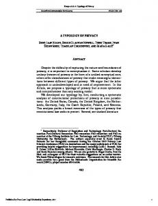
(EQR). One recommended option is to calculate an EQR by dividing an observed metric value by the reference metric value for its lake type (REFCOND, 2003). This yields an EQR that ranges from near 1 (high/reference status) to near 0 (bad status). The overall EQR for a lake is assigned using the lowest EQR recorded for each of the biological elements and the supporting physical and chemical elements. Figure 1.1 shows a summary of the steps necessary for assignment of an EQR.

The key step necessary for the WFD EQR system to work is the development of ecological assessment tools or metrics for each of the biological elements that successfully describe deviation from reference condition along a pressure gradient. Currently, there are no widely accepted ecological assessment tools for any of the biological elements. This was the fourth objective of this project, to carry out developmental work on ecological assessment tools for the biological elements: phytoplankton,

macrophytes,

littoral

macroinvertebrates

and

profundal

macroinvertebrates. Metrics may be developed to work along one or more pressure gradients. This project focused on nutrients, i.e.total phosphorus, as the main pressure affecting Irish lakes.

This project examined a number of ecological assessment approaches depending on their suitability to the biological element under consideration. These included multimetric indices, published indices, simple empirically-based indices and multivariate classification. The different methods are described in the relevant chapters.

The aim of this work is to better position Ireland to meet its commitments to assess lakes ecologically as required by the WFD. The successful ecological assessment of lakes was recognised at an early stage by the Irish EPA to be crucially dependent on research. This is the second EPA commissioned research project on the ecological assessment of lakes: the first by Irvine et al. (2001) was commissioned in 1995. Effective ecological assessment is an enormous challenge that will necessitate constant refinement, through research, for many years to come.

6

1. Define a typology that partitions biological variation in reference condition

Lake type A

Lake type B………..C etc e.g. High Alkalinity, > 4 m mean depth, > 50 ha area

2. Identify and describe type-specific reference conditions

Description of reference condition for lake type A using metric values for the biological elements. Biological element

Phytoplankton Macrophytes

Metric value

0.95

Littoral Profundal invertebrates invertebrates

Phytobenthos

0.94

24

0.93

Fish

1000

0.95

3. Apply assessment metric to measure deviation away from type-specific reference status for each biological element.

0.0 0

1

2 Pressure

3

0.5

0.0 0

1

2 Pressure

1.0 Fish metric

0.5

1.0 Invertebrate metric

1.0 Macrophyte metric

Phytoplankton metric

1.0

0.5

0.0

3

0.5

0.0 0

1

2 Pressure

3

0

1

2 Pressure

4. For each lake, the Ecological Quality Ratio (EQR) is calculated for each element as: observed / reference metric value. Lowest EQR is used for assessment (including a physicochemical EQR – not shown). EQR for Lake X. Scale may range from high status: near 1, to bad status: near 0. Biological element EQR

Phytoplankton Macrophytes 0.71

0.64

Phytobenthos 0.69

Littoral Profundal invertebrates invertebrates 0.74

Fish

0.73

0.80

Figure 1.1 Main steps required by WFD for assignment of an Ecological Quality Ratio (simplified).

7

3

2. Overview of lakes sampled 2.1 Introduction This chapter introduces the lakes sampled and provides details on some of their physico-chemical and hydro-morphological characteristics. In total 201 lakes across the country were sampled between 2001 and 2003. These include a large proportion of the lakes in the country over 50 ha surface area (required by the WFD) as well as a selection of smaller lakes principally located in the midlands and along the western seaboard. Figure 2.1 shows the location of the lakes sampled. Grid references for the locations of the lakes are listed in Table 2.1. There are fewer lakes in the east, southeast and south of the country which accounts for the absence or low number of lakes studied in these areas.

Figure 2.1 Location of the lakes sampled. Candidate reference lakes are indicated by solid circles.

8

2.2. Frequency of sampling The lakes sampled and the dates they were sampled on are listed in Table 2.2. Details of sampling methodology and the biological elements collected can be found in Chapter 3. In Spring 2001, 161 lakes were sampled. These lakes were selected primarily on the basis of size and all, apart from four lakes, had a surface area greater than 50 ha. During the Summer of 2001, 98 of these lakes were sampled again along with an additional 13 lakes. Sampling in 2002 concentrated solely on lakes which were potential reference candidates. Lakes were assessed and chosen on the basis of Geographical Information Systems (GIS) mapping and historical chemical and biological results. In Spring 2002, 69 potential reference lakes were sampled, which included 42 lakes that had been sampled the previous year and an additional 27 lakes. Of these 69 lakes 40 were sampled again during the Summer of 2002. In the Summer of 2003, 57 lakes were sampled. All of these lakes had been sampled once in Spring 2001. As time limitations did not permit them to be sampled in Summer 2001, they were sampled in Summer 2003. Thus, the vast majority of the 201 lakes have been sampled in both Spring and Summer.

2.3 Physical characteristics of the lakes GIS software and a digital elevation model were used to delineate catchments upstream from each lake outflow and to calculate lake and catchment areas and perimeters. Altitude data and the location of the lakes, recorded as Irish Grid Reference, were obtained from the Ordnance Survey “Discovery” Series 1:50 000 scale maps. These data are presented in Table 2.1 for each of the lakes sampled. The National Lake Code is a unique code for each lake in the country and incorporates a Hydrometric Area code, a River Catchment code and a Lake number generated by GIS distance ordering functions based upon a lakes distance from the river mouth.

9

Table 2.1 Physical characteristics of lakes Lake Code 28-00154-0110-000 31-000r4-0260-000 38-00016-0400-000 25-0155b-0350-000 26-0155a-3000-000 19-00228-0240-000 32-t4_32-0760-000 26-0155a-1060-000 38-00022-0060-000 31-000r4-1120-000 35-00116-0360-000 27-00158-0980-000 25-0155b-0370-000 32-000u4-0240-000 36-00123-5280-000 31-00136-0290-000 30-00143-0100-000 27-00158-0770-000 27-00158-1460-000 34-00110-0220-000 32-00004-0120-000 31-000r4-2040-000 07-00159-0930-000 21-00216-0020-000 38-00048-0490-000 35-00117-0170-000 32-00108-0140-000 26-0155a-1640-000 30-00143-1040-000 26-0155a-1450-000 36-00123-1490-000 27-00250-0460-000 27-00158-1760-000 22-00208-0020-000 30-00143-1690-000 19-00228-0070-000 35-00117-0110-000 34-00110-0230-000 33-00105-0030-000 26-0155a-2100-000 21-00220-0030-000 27-00250-0280-000 22-00208-0090-000 31-00138-0130-000 35-00116-0280-000 26-0155a-2210-000 21-00213-0090-000 32-t4_32-0520-000 34-00110-0430-200 26-0155a-0120-000

Lake name

Co.*

National Grid Ref.

Acrow Ahalia North Aleck More Alewnaghta Allen Allua Anaserd Annaghmore Anure Arderry Arrow Atedaun Atorick Aughrusbeg Avaghon Ballinahinch Ballycuirke Ballycullinan Ballyeighter Ballymore Ballynakill Ballynakill (G) Bane Barfinnihy Barra Belhavel Beltra Boderg Bofin Bofin Brackley Bridget Bunny Caragh Carra Carraigadrohid Carrigeencor Carrowkeribly Carrowmore Cavetown Clonee Clonlea Cloon Cloonacleigha Cloonadoon Cloonagh Cloonaghlin Cloongat Conn Coosan

CE GY DL CE LM CK GY RN DL GY SO CE CE GY MN GY GY CE CE MO GY GY WH KY DL LM MO LD GY LD CN CE CE KY MO CK LM MO MO RN KY CE KY SO GY RN KY GY MO WH

R 193 687 L 965 390 B 762 080 R 759 911 G 960 200 W 190 655 L 606 445 M 900 837 B 820 165 L 995 457 G 790 109 R 295 885 R 630 965 L 555 582 H 690 135 L 765 480 M 230 315 R 288 857 R 357 940 G 290 128 L 640 580 L 865 222 N 550 712 V 850 768 B 935 120 G 880 290 M 070 980 N 015 910 M 035 440 N 040 885 H 190 205 R 565 807 R 375 967 V 725 905 M 180 710 W 360 702 G 830 336 G 266 110 F 836 283 M 830 972 V 810 640 R 510 735 V 702 777 G 610 150 M 008 315 M 545 870 V 610 707 L 689 472 G 180 100 N 055 450

Altitude meters 195 2 10 31 47 84 8 46 36 37 53 13 136 8 127 7 6 20 17 15 8 13 112 249 90 60 15 39 40 39 58 30 17 15 20 60 45 8 7 82 26 26 90 57 29 81 109 14 9 35

Lake area km2 0.06 0.39 0.61 0.55 33.56 1.36 0.87 0.53 1.59 0.81 12.47 0.38 0.98 0.50 0.54 1.70 0.74 0.29 0.28 0.56 0.62 0.24 0.75 0.14 0.63 1.01 4.10 5.11 0.92 2.58 1.67 0.55 1.03 4.91 15.64 5.77 0.44 0.51 9.28 0.64 0.71 0.40 0.77 0.62 0.49 0.71 1.28 0.08 48.48 0.56

Catchment area km2 0.30 46.25 7.66 26.25 403.35 109.28 2.08 3.96 37.29 14.42 65.76 176.63 28.92 1.69 3.96 155.23 33.45 10.74 3.17 27.25 7.70 1.41 4.70 0.79 19.68 22.24 96.53 21.90 17.43 4.70 9.32 162.54 108.45 618.97 2.63 34.28 87.95 9.06 27.02 5.91 17.19 32.63 43.56 47.93 10.24 6.06 416.48 4.18

10

Table 2.1 (cont.) Physical characteristics of lakes Lake Code 36-00123-2860-000 30-00143-0570-000 26-0155a-2010-000 16-00182-0210-000 38-00016-0200-000 33-000k5-0160-000 16-00182-0150-000 27-00158-1190-000 27-00158-0750-000 34-00110-0670-000 21-00213-0010-000 29-00146-0010-000 10-00171-0070-000 01-00063-0340-000 25-0155b-0450-000 26-00157-0370-000 36-00123-2530-000 36-00123-1910-000 31-00136-0470-000 34-00110-1110-000 28-00152-0050-000 39-00008-0010-000 32-00130-0020-000 36-00123-4630-000 26-0155a-2290-000 36-00123-1800-000 36-00123-4750-000 27-00250-0330-000 38-00016-0070-000 37- a6_37-0010-000 35-00114-0150-000 36-00123-5970-000 25-0155b-0950-000 26-0155a-2140-000 37-00058-0060-000 40-0000c-0020-000 40-00004-0010-000 32-t4_32-0210-000 32-00132-0020-000 32-00107-0070-000 39-00031-0080-000 32-00130-0010-000 27-00250-0100-000 01-00062-0210-000 26-0155a-0930-000 32-00107-0030-000 26-0155a-2260-000 36-00123-1830-000 39-00031-0270-000 36-00123-3530-000 23-000z3-0010-000 35-00117-0040-000 21-00222-0010-000

Lake name

Co.*

National Grid Ref.

Corglass Corrib Corry Coumduala Craghy Cross Crottys Cullaun Cullaunyheeda Cullin Currane Cutra Dan Derg Derg Derravaragh Derrybrick Derrycassan Derryclare Derryhick Doo Doo Doo Dromore Drumharlow Drumlaheen Drumlona Dúin Dunglow Dunlewy Durnesh Easky Egish Ennell Errit Eske Fad (east) Fad (west) Fadda Fee Feeagh Fern Fin Finn Finn Forbes Furnace Gara Garadice Gartan Garty Gill Gill Glanmore

CN GY RN WD DL MO WD CE CE MO KY GY WW DL TN WH CN CN GY MO CE DL MO CN RN LM MN CE DL DL DL SO MN WH RN DL DL DL FY GY MO DL MO CE DL LD MO RN LM DL CN KY SO KY

H 346 089 M 250 415 M 945 965 S 293 143 B 795 115 F 645 296 S 326 125 R 315 905 R 485 745 G 230 030 V 530 660 R 475 985 O 150 040 H 080 745 R 800 900 N 410 680 H 345 120 H 225 118 L 825 485 M 205 990 R 120 720 C 359 394 L 833 682 H 610 161 G 905 015 H 090 070 H 640 175 R 545 736 B 782 117 B 915 194 G 878 693 G 442 225 H 795 132 N 390 460 M 540 851 G 972 837 C 539 393 C 397 427 L 667 455 L 790 613 F 965 000 C 180 230 L 841 657 R 435 695 B 910 015 N 080 815 L 968 974 M 705 995 H 180 110 C 050 156 N 280 980 Q 610 140 G 750 340 V 775 550

Altitude meters 45 6 41 468 14 3 419 16 27 9 6 33 200 140 30 61 45 45 10 25 83 283 30 79 40 65 77 22 13 61 0 180 161 81 83 27 233 125 13 47 11 20 28 27 132 37 0 66 49 67 67 3 0 8

Lake Catchment area area km2 km2 0.34 1.17 172.91 2954.93 1.54 0.02 0.16 0.50 25.22 1.11 3.37 0.04 0.08 0.50 13.20 1.55 22.99 10.24 802.81 10.35 103.98 3.88 120.95 1.03 63.18 8.81 35.14 122.20 3958.81 9.14 559.23 0.36 1.54 0.71 309.87 2.24 111.73 0.54 9.06 1.30 23.11 0.09 0.43 1.55 27.52 0.61 213.60 2.79 0.74 2.34 0.53 20.34 0.49 36.67 0.61 37.67 1.10 35.96 0.70 15.10 1.19 10.80 1.17 8.72 11.56 117.62 0.82 7.15 3.87 79.65 0.12 0.61 0.40 3.20 0.47 4.40 1.74 15.76 3.95 84.68 1.81 206.17 0.14 30.96 0.74 3.40 1.15 10.61 2.98 1.84 101.86 12.57 499.69 3.89 183.91 2.05 77.44 0.83 20.76 1.40 16.43 13.81 365.62 0.57 24.44

11

Table 2.1 (cont.) Physical characteristics of lakes Lake Code 36-00123-2420-000 38-00027-0010-000 35-00117-0120-000 21-000h3-0040-000 35-00119-0010-000 32-00130-0050-000 31-00136-0490-000 31-00138-0060-000 26-00156-0580-000 26-00157-0650-000 36-00123-0330-000 36-00123-4440-000 25-0155b-0320-000 22-00207-0530-000 36-00123-3060-000 31-000r4-2010-000 31-00136-0520-000 27-00158-1320-000 21-00220-0050-000 19-00228-0170-000 31-000r4-0050-000 34-00110-2390-000 38-00030-0020-000 33-i5_33-0820-000 38-00022-0080-000 26-0155a-2720-000 26-0155a-1260-000 26-0155a-0180-000 38-000j6-0050-000 26-00157-0570-000 38-u6_38-0110-000 32-00125-0020-000 32-00133-0050-000 34-00110-2220-000 07-00159-1150-000 30-00143-0710-000 34-00110-0930-000 28-00149-0080-000 31-00137-0260-000 30-00143-1360-000 36-00123-1070-000 30-00143-1580-000 31-t4_31-0010-000 30-00143-1460-000 38-00016-0110-000 26-0155a-2950-000 35-00121-0010-000 01-00063-0050-000 27-00158-1470-000 06-00094-0280-000 22-00207-0270-000 38-0016-0780-000 26-0155a-1400-000 38-00023-0090-000

Lake name

Co.*

National Grid Ref.

Glasshouse Glen Glenade Glenbeg Glencar Glencullin Glendollagh Glenicmurrin Glinn Glore Golagh Gowna Graney Guitane Gulladoo Hibbert Inagh Inchiquin Inchiquin Inishcarra Invernagleragh Islandeady Keel Keel (Achill) Keel (Rosses) Key Kilglass Killinure Kiltooris Kinale Kindrum Knappabeg Kylemore Lannagh Lene Lettercraffroe Levally Lickeen Loughanillaun Loughanillaun (M) Macnean Mask Maumeen Maumwee Meela Meelagh Melvin Mourne Muckanagh Muckno Muckross Mullaghderg Nablahy Nacung Upper

CN DL LM KY LM MO GY GY RN WH DL LD CE KY CN GY GY CE KY CK GY MO DL MO DL RN RN WH DL CN DL MO GY MO WH GY MO CE GY GY LM MO GY GY DL RN LM DL CE MN KY DL RN DL

H 270 060 C 105 295 G 825 464 V 705 530 G 750 435 L 819 696 L 840 475 M 000 310 M 635 865 N 489 719 G 965 662 N 284 924 R 556 930 W 025 845 N 240 990 L 882 223 L 845 520 R 270 895 V 835 628 W 480 718 L 925 400 M 090 880 C 153 250 F 650 060 B 847 162 G 840 600 M 980 850 N 070 460 G 675 970 N 390 810 C 185 430 M 008 803 L 770 552 M 111 885 N 510 685 M 059 375 G 145 045 R 175 909 L 848 415 L 809 471 H 032 397 M 100 600 L 615 412 L 977 484 B 740 133 G 890 120 G 900 540 H 068 896 R 370 925 H 845 195 V 950 852 B 760 200 M 952 885 B 894 205

Altitude meters 48 24 66 78 28 38 16 28 87 79 101 61 46 77 51 15 25 19 42 40 4 27 97 6 136 42 38 35 7 62 8 30 35 28 93 160 29 70 26 40 50 20 5 46 3 50 25 168 17 86 17 3 40 59

Lake Catchment area area km2 km2 0.54 117.16 1.68 124.22 0.74 15.87 0.66 7.58 1.15 41.22 0.34 6.08 0.83 49.61 1.65 67.05 0.55 2.86 0.24 16.75 0.60 4.59 4.15 129.40 3.72 109.64 2.46 19.03 0.39 82.39 0.25 3.05 3.14 48.08 1.08 135.58 0.77 17.94 4.90 783.79 0.56 11.19 1.39 55.94 0.61 2.60 0.85 12.36 0.11 3.96 8.90 2.02 230.30 2.56 83.12 0.43 5.55 1.95 263.37 0.61 3.67 0.22 18.45 1.32 20.91 0.59 62.46 4.16 12.96 0.82 4.25 1.23 20.18 0.84 9.03 0.57 20.59 0.67 9.19 9.78 120.37 83.43 938.40 0.56 2.28 0.28 3.97 0.57 9.52 1.16 7.04 22.06 183.05 0.67 8.87 0.96 22.15 3.57 109.08 2.67 137.20 0.54 5.60 0.53 104.68 2.08 78.62

12

Table 2.1 (cont.) Physical characteristics of lakes Lake Catchment area area km2 km2 07-00159-1120-000 Nadreegeel CN N 545 930 103 0.44 11.44 30-00143-1660-000 Nafooey GY L 970 595 25 2.48 33.67 31-000q4-0040-000 Nagravin GY L 990 215 14 0.56 5.12 31-000r4-0720-000 Nahasleam GY L 971 440 33 0.28 22.78 22-00208-0060-000 Nakirka KY V 735 892 173 0.06 0.53 37-00052-0120-000 Nalughraman DL G 657 886 180 0.56 2.22 37-00055-0010-000 Namanfin DL G 797 839 128 0.23 1.85 32-00132-0040-000 Nambrackkeagh GY L 821 604 65 0.07 0.56 40-00004-0020-000 Naminn DL C 396 419 150 0.15 1.10 28-00152-0060-000 Naminna CE R 176 710 169 0.20 0.91 26-0155a-2460-000 Oakport RN G 888 036 42 0.51 26-00156-0570-000 O'Flynn RN M 585 795 77 1.37 18.35 31-00136-0670-000 Oorid GY L 930 460 45 0.61 7.40 26-00157-0260-000 Owel WH N 400 580 97 10.22 32.15 09-00168-0230-000 Pollaphuca WW O 000 010 180 19.53 318.67 07-00159-0600-000 Ramor CN N 600 869 82 7.13 234.84 29-00145-0180-000 Rea GY M 615 155 81 3.01 234.84 26-0155a-0320-000 Ree WH N 000 580 35 106.10 4620.07 26-0155a-1770-000 Rinn LM N 100 930 39 1.65 178.06 36-00123-2800-000 Rockfield CN H 272 035 47 0.38 82.39 30-00143-0330-000 Ross GY M 190 365 6 1.39 53.81 26-0155a-2710-000 Rowan LM H 085 060 73 0.48 1.98 26-0155a-1780-000 Sallagh LM N160 912 55 0.49 3.68 38-00027-0110-000 Salt DL C 124 262 246 0.29 1.01 36-00123-1630-000 Scur LM H 027 084 62 1.14 62.87 26-00157-0690-000 Sheelin CN N 450 850 61 18.16 242.16 31-000r4-0950-000 Shindilla GY L 960 460 38 0.70 9.66 36-00123-5720-000 Sillan CN H 700 070 94 1.62 51.26 31-000r4-1600-000 Skannive GY L 809 320 16 0.81 14.62 07-00159-0620-000 Skeagh Upper CN H 650 010 150 0.61 4.09 29-0155a-2950-000 Skean RN G 858 125 48 1.14 78.31 33-i5_33-0660-000 Sruhill MO F 724 085 2 0.51 2.71 36-00123-1640-000 St. Johns LM H 090 100 60 1.46 22.56 26-00157-0040-000 Sunderlin WH N 220 501 77 0.22 2.57 34-00110-0630-000 Talt SO G 398 150 130 0.97 5.70 26-0155a-1810-000 Tap LD N 006 945 39 0.62 10-00171-0090-000 Tay WW O 160 075 250 0.50 20.03 35-00116-0230-000 Templehouse SO G 615 170 54 1.19 268.54 22-00207-0260-000 Upper KY V 900 817 18 1.70 113.08 26-0155a-2400-000 Urlaur MO M 512 888 81 1.15 13.60 38-00027-0210-000 Veagh DL C 017 211 40 2.61 36.88 38-00016-0370-000 Waskel DL B 738 161 3 0.31 3.14 36-00123-4940-000 White MN H 680 188 75 0.54 132.38 * Co.- County: CE – Clare, CK – Cork, CN – Cavan, DL – Donegal, GY – Galway, KY – Kerry, LD Longford, LM – Leitrim, MN – Monaghan, MO – Mayo, RN – Roscommon, SO – Sligo, TN – Tipperary, WD – Waterford, WH – Westmeath, WW – Wicklow. Lake Code

Lake name

Co.*

National Grid Ref.

Altitude meters

13

Table 2.2 Names of lakes and dates sampled. LAKE Acrow Ahalia Aleck More Alewnaghta Allen Allua Anaserd Annaghmore Anure Ardderry Arrow Atedaun Atorick Aughrusbeg Avaghon Ballinahinch Ballycuirke Ballycullinan Ballyeighter Ballymore Ballynakill Ballynakill (Gorumna) Bane Barfinnihy Barra Belhavel Beltra Boderg Bofin Bofin Brackley Bridget Bunny Caragh Carra Carraigadrohid Carrigeencor Carrowkeribly Carrowmore Cavetown Clonee Clonlea Cloon Cloonacleigha Cloonadoon Cloonagh Cloonaghlin Cloongat Conn Coosan Corglass Corrib Corry

Co.* CE GY DL CE LM CK GY RN DL GY SO CE CE GY MN GY GY CE CE MO GY GY WH KY DL LM MO LD GY LD CN CE CE KY MO CK LM MO MO RN KY CE KY SO GY RN KY GY MO WH CN GY RN

Spring 2001 29/05/01 02/05/01 27/04/01 05/06/01 15/05/01 09/05/01 11/06/01 02/05/01 24/04/01 28/06/01 31/03/01 29/03/01 09/05/01 07/06/01 08/05/01 29/05/01 02/04/01 25/04/01 04/04/01 10/05/01

Summer 2001

Summer 2003

22/08/03 17/08/01 30/07/03 25/07/01 01/08/01

30/04/02 17/04/02 22/04/02

13/09/02 14/08/02 30/07/02

03/08/01 10/08/01 31/07/03 31/08/01 05/09/01 03/09/01 30/07/03 31/07/03 22/08/01 31/07/03 24/08/01

23/05/01 29/06/01 01/06/01

26/07/01

16/06/01 23/04/01 06/04/01 30/04/01 17/05/01 15/05/01 30/06/01 03/04/01 09/04/01 13/06/01 17/05/01 24/04/01 30/04/01 19/04/01

Summer 2002 04/09/02

24/07/01

24/05/01

24/04/01

Spring 2002 18/04/02

23/04/02 09/04/02 24/04/02 11/04/02

06/08/02 11/09/02 16/08/02 15/08/02

08/05/02

27/08/02

24/07/03 16/08/01 04/07/01 30/07/01 05/07/01 31/07/01 04/08/01

20/08/03 20/08/03 06/08/03 16/04/02 25/04/02

03/09/02 15/08/02

24/07/03 22/08/01 09/08/01 16/08/01 31/07/03 13/08/01

25/04/02

16/08/02 11/08/03

31/07/01 11/04/01

12/08/03 26/04/02 24/04/02

21/08/02 07/08/02

14/05/01 03/07/01 15/06/01 25/05/01 14/06/01

21/08/03 05/08/03 05/06/02

21/08/02 13/08/03

14

Table 2.2 (Cont.) Names of lakes and dates sampled. LAKE Coumduala Craghy Cross Crotty Cullaun Cullaunyheeda Cullin Currane Cutra Dan Derg Derg Derravaragh Derrybrick Derrycassen Derryclare Derryhick Doo Doo Doo Dromore Drumharlow Drumlaheen Drumlona Dúin Dunglow Dunlewy Durnesh Easky Egish Ennell Errit Eske Fad (east) Fad (west) Fadda Fee Feeagh Fern Fin MO Finn Finn Forbes Furnace Gara Garadice Gartan Garty Gill Gill Glanmore Glasshouse Glen Glenade Glenbeg Glencar Glencullin Glendollagh Glenicmurren Glinn

Co.* WD DL MO WD CE CE MO KY GY WW DL TN WH CN CN GY MO CE DL MO CN RN LM MN CE DL DL DL SO MN WH RN DL DL DL GY GY MO DL MO CE DL LD MO RN LM DL CN KY SO KY CN DL LM KY LM MO GY GY RN

Spring 2001

Summer 2001

01/05/01 09/04/01

24/07/01

02/04/01 25/04/01 03/04/01 01/05/01 28/03/01 19/04/01 05/06/01 23/05/01 16/06/01 20/06/01 30/05/01 30/03/01 04/04/01 06/04/01 09/06/01 14/06/01 18/06/01 08/06/01 24/04/01 01/05/01 03/05/01 06/06/01 18/04/01 08/06/01 22/05/01 10/04/01 05/06/01

30/05/01 18/05/01 21/05/01 30/03/01 23/05/01

Spring 2002 22/05/02 16/04/02

Summer 2002

Summer 2003

13/08/02 01/09/03

05/08/01 01/08/01 14/05/01

22/05/02 17/04/02

18/07/02

26/04/02

20/08/02

19/04/02

07/08/02

29/07/03 28/08/01

05/08/03 10/07/01 22/08/01 06/09/01 06/09/01 30/07/03 23/07/03 10/04/02 02/05/02

22/07/02 03/09/02 07/08/03 20/08/03

16/09/01 30/08/01 30/07/01 24/07/01

16/04/02

13/08/02 07/08/03

15/08/01

07/05/02

28/08/02 10/07/03

25/08/01 14/08/01 29/08/01 05/09/01 02/08/01

18/04/02 18/04/02

23/07/02 23/07/02

25/04/02 08/05/02

08/08/02 27/08/02

02/05/02

03/09/02

27/08/01 02/08/01 28/08/01 05/07/01

19/08/03

18/05/01 29/06/01 22/05/01 14/06/01 28/04/01 28/06/01 18/05/01 09/06/01 22/05/01 27/06/01 18/05/01 27/06/01 08/05/01 28/05/01 11/04/01

03/07/01 25/07/01 05/09/01 15/08/01 04/09/01 26/07/01 30/08/01 15/08/01 30/08/01

13/08/03 11/04/02

15/08/02

12/04/02 02/05/02

30/07/02 29/08/02

06/09/01 31/07/01

15

Table 2.2 (Cont.) Names of lakes and dates sampled. LAKE

Co.*

Glore Golagh Gowna Graney Guitane Gulladoo Hibbert Inagh Inchiquin Inchiquin Inishcarra Invernagleragh Islandeady Keel Keel (Achill) Keel (Rosses) Key Kilglass Killinure Kiltooris Kinale Kindrum Knappabeg Kylemore Lannagh Lene Lettercraffoe Levally Lickeen Loughanillaun Loughanillaun (Maam) Mask Maumeen Maumwee Macnean Meela Meelagh Melvin Mourne Muckanagh Muckno Muckross Mullaghderg Nablahy Nacung Upper Nadreegel Nafooey Nagravin Nahasleam Nakirka Nalughraman Namanfin Nambrackkeagh Naminn Naminna Oakport O'Flynn Oorid Owel

WH DL LD CE KY CN GY GY CE KY CK GY MO DL MO DL RN RN WH DL CN DL MO GY MO WH GY MO CE GY GY MO GY GY LM DL RN SO DL CE MN KY DL RN DL CN GY GY GY KY DL DL GY DL CE RN RN GY WH

Spring 2001 24/05/01 06/06/01 30/05/01 29/03/01 16/05/01 15/06/01 08/05/01 05/04/01 17/05/01 14/05/01 25/04/01 29/03/01 21/05/01 15/05/01

Summer 2001

Spring 2002

Summer 2002

11/04/02

01/08/02

22/07/03 23/07/03 09/08/01 14/08/01 05/09/01 04/09/01 10/08/01 14/08/01

23/04/02

19/07/02

23/04/02

06/08/02

27/04/02

06/09/02 22/07/03

27/08/01 24/07/03 16/04/02

14/08/02

28/06/01 14/06/01

14/08/03 20/08/03 03/09/03

03/07/01 30/04/01 27/06/01 21/05/01 10/05/01 01/06/01 23/05/01 28/05/01 30/03/01 31/03/01 25/04/01 23/04/01 23/04/01 01/05/01 13/06/01 27/06/01 02/04/01 13/06/01 02/05/01 11/06/01 02/05/01 29/05/01 30/05/01 28/05/01 30/04/01

28/06/01 11/06/01 24/04/01 23/05/01

Summer 2003

15/04/02

12/08/02

28/08/01 03/07/01 02/08/01

10/04/02

24/07/02

24/04/02

07/08/02

24/08/01 03/09/01 23/08/01 11/08/01 31/07/01

09/04/02

26/07/02

01/05/02 24/04/02 22/04/02 10/04/02

20/08/02 07/08/02 29/07/02 02/08/02

11/08/03 23/07/03 22/07/03

29/07/03 30/07/01 09/07/01

06/08/03 08/08/01 11/09/01 04/08/01

10/04/02 11/04/02 17/04/02

31/07/02 03/08/02 03/09/02

23/04/02

22/08/02

11/07/03 06/08/03 09/08/01 07/08/03 31/08/01 06/09/01

25/04/02

26/08/02

23/04/02 25/04/02 15/04/02 15/04/02 25/04/02 17/04/02 17/04/02

30/07/02 14/08/02

30/04/02 22/04/02 08/04/02

12/09/02 29/07/02 25/07/02

28/07/03 23/07/01

12/08/02 26/08/02 23/07/02 04/09/02 21/08/03

14/08/01 01/08/01 23/08/01

16

Table 2.2 (Cont.) Names of lakes and dates sampled. LAKE

Co.*

Pollaphuca Ramor Rea Ree Rinn Rockfield Ross Rowan Sallagh Salt Scur Sheelin Shindilla Sillan Skannive Skeagh Skean Sruhill St. Johns Sunderlin Talt Tap Tay Templehouse Upper Urlar Veagh Waskel White

WW CN GY WH LM CN GY LM LM DL LM CN GY CN GY CN RN MO LM WH SO LD WW SO KY MO DL DL MN

Spring 2001

Summer 2001

11/04/01 31/05/01 27/03/01

Spring 2002

Summer 2002

Summer 2003 15/07/03 09/07/03

16/04/02

02/09/02

12/07/01 28/06/01 10/06/01 29/05/01 18/06/01 28/06/01 29/06/01 27/06/01 24/04/01 06/06/01 25/04/01 29/05/01 13/06/01 15/05/01 20/06/01 25/05/01 18/04/01

18/07/03 04/09/01 29/07/03 16/09/01 17/07/03 10/04/02

23/07/02

22/04/02

31/07/02

15/09/01 12/08/03 04/09/01 29/08/01

28/07/03 29/08/01 08/08/01 14/08/03 18/08/03 15/08/01 04/07/01

07/05/02

28/08/02

19/04/02

07/08/02

24/04/02

05/09/02

17/04/02 16/04/02

16/07/02 13/08/02

02/09/03

19/04/01 10/04/01 22/05/01 01/05/01 07/06/01

11/08/03 07/08/01

12/08/03

30/08/01

* Co.- County: CE – Clare, CK – Cork, CN – Cavan, DL – Donegal, GY – Galway, KY – Kerry, LD Longford, LM – Leitrim, MN – Monaghan, MO – Mayo, RN – Roscommon, SO – Sligo, TN – Tipperary, WD – Waterford, WH – Westmeath, WW – Wicklow.

17

2.4 Chemical characteristics of the lakes The 201 lakes sampled represented a wide selection across the physico-chemical and trophic gradients typically found in Ireland. Table 2.3 presents some basic chemistry data for each lake from a single date. Details of the sampling methodology can be found in Chapter 3.

-0.4 6.4 0.9 69.7 n/a 15.0 11.2 159.4 12.5 6.1 120.3 169.4 4.2 54.1 38.6 5.0 69.1 227.6 211.0 104.7 22.4 20.0 132.5 4.2 3.8 12.4 19.4 77.7 6.9 80.3 46.6 200.0 156.2 3.6 172.6 36.0

61 41 186 57 n/a 27 16 19 56 40 10 26 148 32 13 32 44 15 27 44 22 20 1 3 45 156 n/a 54 18 48 55 55 9 23 14 22

0.9 n/a 0.5 1.2 n/a 2.4 2.5** n/a 1.8 1.3 3.2 1.6** 0.8 1.8 3.9 3.3 1.4 2.4 3.4 2.5 3.2 3.2 7.8 4.8 3.2 0.3 2.5 1.3 1.9 1.7 0.9 1.3 5.4 2.8 4.7 n/a

Chlorophyll a µg l-1

73 197 90 202 n/a 78 183 351 70 84 283 379 61 380 160 75 206 481 462 281 145 244 297 56 54 79 99 212 73 216 133 444 361 70 396 130

6.2 3.4 17.4 14.5 4.0 14.1 0.7 0.4 3.4 2.0 6.1 2.4 4.8 13.4 3.2 2.6 13.9 29.8 3.2 3.8 2.6 9.4 1.4 3.2 1.1 9.3 2.6 10.1 1.6 2.8 14.9 26.2 1.4 4.0 1.0 5.2

Total Nitrogen mg l-1

5.14 6.80 4.77 8.00 n/a 7.40 6.74 8.46 6.57 6.33 8.58 8.28 6.45 8.25 7.92 6.27 7.79 8.38 8.42 8.17 7.18 7.1 8.43 6.84 6.31 7.25 7.39 8.01 6.62 8.15 8.03 8.21 8.47 6.73 8.34 7.46

Total Phosphorus µg l-1

18/04/02 29/05/01 02/05/01 27/04/01 05/06/01 15/05/01 09/05/01 30/04/02 02/05/01 24/04/01 28/06/01 31/03/01 29/03/01 09/05/01 07/06/01 08/05/01 29/05/01 02/04/01 25/04/01 04/04/01 10/05/01 23/04/02 09/04/02 24/04/02 23/05/01 29/06/01 01/06/01 04/07/01 24/04/01 05/07/01 16/06/01 23/04/01 16/04/02 30/04/01 17/05/01 15/05/01

pH

Secchi depth meters

CE GY DL CE LM CK GY RN DL GY SO CE CE GY MN GY GY CE CE MO GY GY WH KY DL LM MO LD GY LD CN CE CE KY MO CK

Date sampled

Colour PtCo/Hazen

Acrow Ahalia (North) Aleck More Alewnaghta Allen Allua Anaserd Annaghmore Anure Ardderry Arrow Atedaun Atorick Aughrusbeg Avaghon Ballinahinch Ballycuirke Ballycullinan Ballyeighter Ballymore Ballynakill Ballynakill (Gor) Bane Barfinnihy Barra Belhavel Beltra Boderg Bofin Bofin Brackley Bridget Bunny Caragh Carra Carraigadrohid

Co.†

Alkalinity mg l-1 CaCO3

Lake

Conductivity µS cm-1

Table 2.3. Chemical characteristics of the lakes as measured from a single mid-lake sample collected in 2001 or 2002.

18 26 20 29 102 11 12 6 20 20 19 30 27 37 75 10 30 25 5 40 17 12 5 4 7 74 14 31 10 21 33 27 5 9 19 17

0.30 1 m) taxa (RF%)

5.2.5 Analysis The methods used in data analysis are described in Chapter 3. Analysis was performed on submerged and floating species as defined by Palmer et al. (1992). 69

5.3 Results 5.3.1 General description of macrophytes found in reference lakes A total of 47 submerged and floating (as defined by Palmer et al., 1992) macrophyte taxa were identified from the 58 canidate reference lakes. The average number of taxa found in a lake was 9; the maximum was 16 and the minimum 2 (Figure 5.3). Littorella uniflora was the most ubiquitous, occurring in 97% of the reference lakes. Twenty-eight percent of the taxa were rarely encountered, occurring in less than 5% of the reference lakes. The occurrence and abundance of many macrophyte taxa was strongly influenced by alkalinity. Figure 5.4 shows the relative frequency of selected macrophytes for low, medium and high alkalinity lakes. Angiosperms and Isoetes spp. were the most frequently encountered macrophytes in low alkalinity lakes (< 20 mg l-1 CaCO3). At intermediate alkalinity (20-100 mg l-1 CaCO3) Isoetes spp. were less frequent whereas Chara spp. and Nitella spp. were more frequent. In high alkalinity ‘marl’ lakes (> 100 mg l-1 CaCO3) Chara spp. dominated the reference lakes sampled.

10

100 Bryophytes

90 80

Nitella

70 Frequency % .

Number of lakes .

8

6

4

C hara

60 50

Isoetes

40 30

2

0

20

Angiosperms (Potamogeton)

10

Angiosperms

0 0

5

10

15

Number of taxa found

Figure 5.3 Histogram of number of taxa found in reference lakes.

100

-1

Alkalinity mg l CaCO 3

Figure 5.4 Relative frequency (%) of selected macrophyte groups in 58 reference lakes by alkalinity band.

70

5.3.2 Development of a typology using macrophyte composition and abundance The approach taken to develop the typology had the following objectives: 1) To determine if distinct types were evident in macrophyte community composition and abundance using 58 reference lakes. 2) To see if such ‘biological types’ were also distinct in terms of measured environmental variables. 3) To assign environmental boundaries that are useful in defining distinct biological types. 4) To test and describe the resulting lake types in reference condition.

In order to perform an initial search for biological types; cluster analysis was carried out on transformed (x0.5) macrophyte abundance (g) (Figure 5.5). An indicator species analysis was used to prune the dendrogram to six clusters. Figure 5.6 shows that six clusters had a high number of significant indicator species (11) and that over all taxa the indicator values were most significant (minimum p) between the six clusters. In order to support the findings of the cluster analysis, a non-metric multidimensional scaling (NMS) ordination was carried out using the Sorensen (Bray-Curtis) distance measure. Figure 5.7 shows that four clusters (same symbols as Figure 5.5 encircled) were reasonably well separated along the most important axes (2 and 3) and two clusters were more distinct along axis 1. Using two multivariate techniques like this provides confidence that the underlying biological variation has been adequately represented by the cluster analysis.

The next step was to see if the six clusters were distinct in terms of macrophytes and measured environmental variables. To do this, an indicator species analysis was carried out on the six clusters to identify taxa that were significant indicators of a cluster in terms of macrophyte abundance and composition (Table 5.3). In order to visualise differences in environmental variables between clusters, box-plots were drawn (Figure 4.4). Pair-wise post-hoc tests (with Bonferroni adjustment) identified where these differences were significant (Table 5.4). Table 5.5 provides a brief description of the clusters with reference to Table 5.3, Figure 5.8 and Table 5.4.

71

Distance (Objective Function) 7.6E-04

3.4E+00

100

75

6.9E+00

1E+01

1.4E+01

25

0

Information Remaining (%) 50

Acrow Beltra Golagh Dan Tay Arderry Fee Feeagh Craghy Waskel Fad(InW) Doo(MO) Cloon Cloonagh Anure Nafooey Naminna Kylemore Fad(InE) McNean Melvin Doo(DL) Dunglow Shindill Veagh Currane Guitane Muckross Easky Mourne BallynaG Kiltoori Glencull Oorid Nambrack Cloongat Nahaslea Hibbert Maumw ee Barfinni Maumeen Glencar Inch(KY) Upper Caragh Nakirka Annag Bunny Lene Ow el Rea Muckanag Bane Cullaun O'Flynn Naminn Talt Kindrum

Figure 5.5 Dendrogram from cluster analysis of transformed (x0.5) macrophyte abundance in reference lakes (n = 58). Sorensen (Bray-Curtis) distance measure was used with flexible beta (-0.25) linkage. Dashed line represents cut-off point for six clusters.

Average p

12 10

0.3

8

0.2

6 4

0.1

2 minimum p

0.0 0

5

Significant indicators.

14

0.4

0

10

15

Number of clusters Figure 5.6 Average p for all taxa (○) and number of significant (p < 0.05) indicator species identified (●) from an indicator species analysis of clusters 2 to 13. Minimum p (0.10) was reached after six clusters.

72

1

1

0.5

0.5

Axis 1

1.5

Axis 3

1.5

Axis 3

Axis 2 0

0 -1.5

-1

-0.5

0

0.5

1

1.5

-1.5

-1

-0.5

0

-0.5

-0.5

-1

-1

-1.5

-1.5

1

1.5

Axis 1

1.5

0.5

1

0.5

Axis 2

0 -1.5

-1

-0.5

0

0.5

1

1.5

-0.5

-1

-1.5

Figure 5.7 NMS ordination of transformed (x0.5) macrophyte abundance (g) in reference lakes (n = 58). Sorensen (Bray-Curtis) distance measure used; stress: 17.8. The proportion of variance explained by axis 2 was 35%, axis 3: 22% and axis 1: 13%. Symbols and overlays identify the six clusters found in Figure 5.5.

73

Table 5.3 Taxa that were found to be significant indicators of clusters. %F = % frequency of occurrence in cluster, %RA = % relative abundance in cluster. p was determined by Monte Carlo test - proportion of 1000 randomised trials where the observed indicator value was equalled or exceeded (McCune et al., 2002).

Alkalinity

2 2 3 4 4 4 4 4 4 5 5 5

Colour

Altitude m

Depth m

Chara spp. Elodea canadensis Myriophyllum alterniflorum Eriocaulon septangulare Isoetes lacustris Lobelia dortmanna Littorella uniflora Myriophyllum spicatum Juncus bulbosus filamentous algae Nitella spp. Potamogeton perfoliatus

70 33 53 88 69 65 63 33 42 66 80 39

%F

%RA

100 33 91 89 100 78 89 33 78 71 86 43

70 100 58 99 69 84 71 97 54 93 93 91

p 0.001 0.038 0.002 0.001 0.001 0.002 0.014 0.024 0.030 0.001 0.001 0.032

Log area

Cluster taxa Indicator indicative of value (%)

Light

Taxa

Figure 5.8 Box plots of clusters by mean transect depth (m), alkalinity (mg l-1 CaCO3), log area (m2), altitude (m), colour (mg l-1 PtCo) and predicted % light remaining at mean transect depth in reference condition (Free et al., 2005). See Figure 5.17 for legend.

74

Table 5.4 Results (p) of Bonferroni post-hoc tests for significance differences between clusters in transformed (Log x + 2) environmental variables. Mean transect Alkalinity mg l-1 Cluster depth m CaCO3 2-1 3-1 3-2 4-1 4-2 4-3 5-1 5-2 5-3 5-4 6-1 6-2 6-3 6-4 6-5

0.112 0.998 0.802 0.007 0.988 0.142 0.955 0.011 0.469 0.001 1.000 0.567 1.000 0.106 0.990

< 0.001 0.906 < 0.001 0.901 < 0.001 1.000 0.993 < 0.001 1.000 1.000 1.000 < 0.001 0.996 0.995 1.000

Area m2 1.000 1.000 1.000 0.325 0.101 0.115 1.000 0.997 0.998 0.885 0.853 0.994 0.995 0.031 0.725

Altitude Colour mg l-1 m PtCo 1.000 1.000 1.000 0.901 0.931 0.894 1.000 1.000 1.000 1.000 1.000 1.000 1.000 0.993 1.000

% light at mean transect depth

< 0.001 1.000 0.002 0.625 0.375 0.803 0.312 0.891 0.475 1.000 0.942 0.535 0.980 1.000 1.000

< 0.001 1.000 < 0.001 < 0.001 1.000 < 0.001 1.000 < 0.001 1.000 < 0.001 0.998 0.006 1.000 0.006 1.000

Table 5.5 Description of clusters using Table 5.3, Table 5.4 and Figure 5.8. Cluster

Description

Cluster 1 (●)

Low alkalinity (median = 4 mg l-1 CaCO3) of medium transect depth (x = 4.2 m) with no significant indicator taxa but consistently had Isoetes lacustris, Litorella uniflora and Fontanalis antipyretica in low abundance. Cluster 2 (○) Alkalinity was significantly higher than all other clusters (median = 131 mg l-1 CaCO3), mean depth was variable, colour was significantly lower than 2 other clusters. Chara spp. and Elodea canadensis were significant indicator taxa. Chara spp. occurred in 100% of this clusters lakes and the majority (70%) of the abundance of Chara spp. in the 58 reference lakes was concentrated into this cluster (Table 5.3). Cluster 3 (▲) Low alkalinity (median = 6 mg l-1 CaCO3) of medium transect depth (x = 3.3 m) with Myriophyllum alterniflorum as a significant indicator taxa occurring in 91% of lakes in this cluster. Cluster 4 ( ) Low alkalinity (median = 6 mg l-1 CaCO3) with a shallow transect depth (x = 1.6 m) that was significantly shallower than 2 other clusters, and had higher estimated light levels (Figure 5.8). Significant indicators were Eriocaulon septangulare, Lobelia dortmanna, Isoetes lacustris, Litorella uniflora, Juncus bulbosus and Myriophyllum spicatum. In addition to these taxa being frequent in this cluster there was also a notable concentration of abundance into this group (Table 5.3 and Table 5.4). Cluster 5 (■) Low alkalinity (median = 3 mg l-1 CaCO3) with a deep transect depth (x = 5.5 m) that was significantly deeper than 2 other clusters. Nitella spp., filamentous algae and Potamogeton perfoliatus were significant indicator taxa. -1 Cluster 6 (□) Low alkalinity (median = 4 mg l CaCO3) with a medium transect depth (x = 4.2 m) and tended to have a higher lake area (Figure 5.8). No significant indicator taxa

were found, both diversity and abundance were low in this cluster.

75

Table 5.4 shows that no significant differences were found in the selected environmental variables among clusters 1, 3, 5 and 6. These groups could all be classified as having low alkalinity lakes with a medium to deep transect depth. In contrast, clusters 2 and 4 had a number of significant differences with the other clusters in terms of environmental variables as well as indicator species (Table 5.3, Table 5.4). Cluster 4 had a low alkalinity but appears distinct from the other lakes of low alkalinity by having a shallow transect depth, high light level and several Isoetid growth forms as significant indicator species. Cluster 2 had a significantly higher alkalinity and its most important indicator taxa were Chara spp.. It is noteworthy that there were few significant differences between the clusters for altitude, colour and lake area (Table 5.4).

Examining the differences in environmental factors between clusters is useful in that factors that exert a strong influence on the biological groups may be readily identified (e.g. alkalinity, Figure 5.8). However, it must also be considered that environmental factors may have compounding effects resulting in a distinct environmental type that is reflected in macrophyte abundance and composition. For example, it may be expected that a combination of low colour, a shallow littoral and a small lake area may lead to a higher abundance of macrophyte taxa by reduced exposure and high light levels (Figure 5.8, Cluster 4). One way to examine clusters in terms of a combination of environmental variables is to perform a discriminant analysis – also known as canonical variates analysis (CVA). CVA determines which linear combination of environmental factors discriminates best between clusters and can indicate if clusters are different in terms of environmental factors (ter Braak and Smilauer, 2002).

Axes 1 and 2 of the CVA represented 80% of the variation in the relationship between clusters (referred to as species in CVA) and the environment (Table 5.6). Figure 5.9 shows the group centroids for each cluster. In support of the univariate examination of environmental variables, the group centroids for clusters 1, 3, 5 and 6 are located close together indicating that they are not distinct environmentally. In contrast, the centroids for clusters 4 and 2 are more distinct and are more closely surrounded by each clusters lakes (encircled). The arrows (Figure 5.9, Figure 5.10) and standardised canonical coefficients (Table 5.7) give an indication of the relative importance of each 76

environmental factor in cluster separation. Alkalinity, area and mean transect depth were the most important discriminant factors along axis 1, 2 and 3 respectively. In contrast, colour and altitude were not found to be significant (p > 0.05) in separating clusters in the model (Table 5.8).

In summary, the analysis of 58 reference lakes indicates that 3 groups were distinct in terms of both macrophytes and environmental characteristics. The first is a high alkalinity group characterised by Chara sp. (cluster 2), the second is a low alkalinity shallow type characterised by rich growth of several Isoetid growth forms (cluster 4). The third group are low alkalinity lakes of medium to deep depth comprising clusters 1, 3, 5 and 6, which although they had some biological differences (Table 5.5) were not clearly distinct environmentally. Alkalinity, area and mean transect depth were the most important factors separating clusters and will be used to form type boundaries.

Selection of lake type boundaries

Environmental type boundaries must be defined in order to separate types of lakes that are distinct biologically. Although the preceding analysis was useful in defining some types and the environmental factors that were important in this, some potential types were underrepresented in reference site selection. For example, only four moderate alkalinity lakes (30 – 100 mg l-1 CaCO3) were included owing to the unavailability of reference conditions over this alkalinity range. However, in terms of defining boundaries, the reference sites available may allow upper and lower alkalinity boundaries to be set which are relevant to macrophytes. Plant communities of low nutrient status lakes may be characterised by Chara species in hard-water lakes and Isoetes species in soft-water lakes (Rørslett and Brettum, 1989; John et al., 1982). In fact, for the two clusters visible in Figure 5.5 (distance 1.3E+01) these taxa had the strongest indicator values (Chara sp. IV = 93%, p = 0.001; Isoetes lacustris IV = 71%, p = 0.003). The distribution of such key taxa may be useful in defining type boundaries. Figure 5.11 shows the frequency of occurrence of Isoetes lacustris and Chara species in relation to alkalinity for 100 lakes with summer total phosphorus

less than 20 µg l-1.

77

4 Axis 2

Gp4

Gp5

Gp1 Colour Gp6 Gp3

Gp2

Altitude

Alkalinity

-3

Depth Area

-4

6

Axis 1

3

Figure 5.9 Axis 1 and 2 of CVA plot of six clusters identified in Figure 5.5. Group centroids ( ) are labelled. Groups 2 and 4 are encircled.

Depth

Axis 3

Gp5

Gp1 Gp6

Gp2 Gp3

Gp4 Altitude Area

Alkalinity

-3

Colour

-4

Axis 1

6

Figure 5.10 Axis 1 and 3 of CVA plot of six clusters identified in Figure 5.5. Group centroids ( ) are labelled.

78

Table 5.6 Summary statistics of CVA axes. Axis 1 Eigenvalues Species-environment correlations Cumulative percentage variance of species data of species-environment relation

Axis 2

0.783 0.885

Axis 3

0.394 0.627

15.7 53.5

23.5 80.4

Axis 4

0.197 0.444 27.5 93.8

0.090 0.300 29.3 100

Table 5.7 Standardised canonical coefficients for transformed (Log x + 2) variables.

Depth Alkalinity Altitude Area Colour

Axis 1

Axis 2

Axis 3

Axis 4

-0.284 1.922 0.404 -0.592 -0.505

-0.619 -0.561 -0.632 -0.825 -0.439

1.144 0.367 -0.494 -0.744 -0.252

-0.392 -0.876 0.051 0.663 -1.080

Table 5.8 Summary of automatic forward selection in CVA. Marginal effects lists variables in order of variance explained by each variable alone. Conditional effects lists variables in order of inclusion in model along with additional variation explained and whether it was significant (p ≤ 0.05). Variables were transformed (Log x + 2).

Marginal Effects Variable Alkalinity Transect depth Colour Area Altitude

Lambda-1 0.67 0.35 0.34 0.21 0.06

Variable

Conditional Effects Lambda-A p

Alkalinity Transect depth Area Colour Altitude

0.67 0.29 0.22 0.15 0.13

0.002 0.006 0.006 0.074 0.084

F 8.61 3.94 3.19 2.13 2.00

79

100

45

90

40

80

35

70

30

60

25

50

20

40

15

30

10

20

5

10

0

0

-5

-5

20

45

70

95

120

145

170

195

220

-10

-1

Alkalinity mg l CaCO 3

Figure 5.11 Percentage frequency of occurrence with fitted smoothed line for Isoetes lacustris (×,──) and Chara (○,─ ─) against alkalinity in lakes with summer TP < 20 µg l-1 (n = 100). Lowess smoothed line was fitted (Velleman, 1997). Isoetes lacustris tends to be largely absent when alkalinity is greater than 20 mg l-1

CaCO3 whereas Chara species increase markedly between 85 and 100 mg l-1 CaCO3. These levels also broadly correspond to the upper 25th percentile alkalinity found in siliceous catchments (26 mg l-1 CaCO3) and the lower 25th percentile (108 mg l-1 CaCO3) found in catchments with 100% limestone (Free et al., 2005). Therefore alkalinities of 20 and 100 mg l-1 CaCO3 may be useful for defining biological and environmental types for Irish lakes. This would effectively leave a third type (20-100 mg l-1 CaCO3) by default. There may be some biological support for this default type. Lakes in this alkalinity band have previously shown some separation in an NMS ordination of macrophyte abundance (Free et al., 2005).

In order to select a type boundary for depth, an average was calculated between the upper and lower 25th percentiles of two shallow clusters (3 and 4) as 2.2 m (Figure 5.8). Cluster 4 was chosen, as it appeared to be strongly influenced by depth in having a distinctly higher amount of littoral rosette species. For the purposes of a reporting typology it was necessary to convert the mean transect depth of 2.2 m into a mean lake depth of 4 m using equation 5.1.

80

% Frequency of Chara .

% Frequency of Isoetes .

50

Mean lake depth = 1.526 + 1.168 · mean transect depth Equation (5.1) 2 (r = 0.61, p = 0.0002, n = 17) mean depth data from Irvine et al. (2001)

The type boundary for lake area was selected as 50 ha based on the Water Framework Directive System A (CEC, 2000). An additional reason was that cluster 4, whose macrophytes may have been influenced by lake area (Figure 5.9, group centroid 4 at opposite end of area vector) were mostly smaller than 50 ha (upper 25th percentile = 37 ha).

Testing the proposed typology and comparing it with the system A typology

In order to determine if the proposed typology above resulted in types that were biologically distinct, pair-wise multi-response permutation procedure (MRPP) tests were carried out on macrophyte abundance. Table 5.9 shows the A values (chancecorrected within-group agreement) of the pair-wise tests. The A values indicate the homogeneity within a group to that expected by chance: 1 equals complete within group homogeneity whereas an A of 0 equals within group heterogeneity equal to that expected by chance (McCune et al., 2002). The main groups previously found to be distinct following CVA and cluster analysis were largely encompassed by the typology and again found to have significant differences in macrophytes (Figure 5.12). For example, cluster 4 is largely (67%) represented in the type “< 20 mg l-1 CaCO3 alkalinity, < 4 m mean depth, 100 mg l-1 CaCO3) lake types tested were found to be significantly different from all the low alkalinity (< 20 mg l-1 CaCO3) lake types. Mid alkalinity lakes (20 - 100 mg l-1 CaCO3) were not found to cluster separately in earlier analysis; however, the MRPP analysis did show evidence for significant differences with most of the low and high alkalinity lake types (Table 5.9). Several of the types in the moderatealkalinity range were underrepresented owing to the unavailability of reference conditions.

The Water Framework Directive requires that typologies developed by member states must achieve at least the same degree of differentiation as would the application of the default system A typology (CEC, 2000). A detailed statistical comparison of both typology systems would be difficult, but only a broad comparison is required

81

(REFCOND, 2003). MRPP tests may allow some comparison of the proposed typology with that of system A (Table 5.9 and Table 5.10). An indication of the degree of differentiation achieved by each typology system is given by comparing the overall A values from the MRPP analysis. The proposed typology for macrophytes had an overall A value of 0.35 (p < 0.001) whereas the default system A typology had an overall A of 0.21 (p < 0.001). This provides some evidence that the biologically derived typology was better at partitioning natural variation than the default system A typology. Comparing Table 5.9 with Table 5.10 it can also be seen that the proposed typology was more successful at partitioning variation in reference macrophyte communities in soft water lakes than system A.

Figure 5.12 Figure 5.9 redrawn with smoothed lines of proposed typology overlain. Axis 1 and 2 of CVA plot of six clusters identified. Group centroids ( ) are labelled.

82

< 20 alk < 4 m < 50 ha < 20 alk < 4 m > 50 ha < 20 alk > 4 m < 50 ha < 20 alk > 4 m > 50 ha 20 - 100 alk < 4 m < 50 ha 20 - 100 alk < 4 m > 50 ha 20 - 100 alk > 4 m < 50 ha 20 - 100 alk > 4 m > 50 ha >100 alk < 4 m < 50 ha >100 alk < 4 m > 50 ha >100 alk > 4 m < 50 ha >100 alk > 4 m > 50 ha

8 4 9 21 1 0 1 5 0 6 1 2

0.13 0.12 0.03 0.11 -0.01

0.01

0.27

0.19

0.13

0.13

0.42

0.35

0.45

0.36

0.26

0.33

0.37

0.32

0.18

0.10

>100 alk > 4 m > 50 ha

>100 alk > 4 m < 50 ha

>100 alk < 4 m > 50 ha

>100 alk < 4 m < 50 ha

20 -100 alk > 4 m > 50 ha

20 -100 alk > 4 m < 50 ha

20 -100 alk < 4 m > 50 ha

20 -100 alk < 4 m < 50 ha

< 20 alk > 4 m > 50 ha

< 20 alk > 4 m < 50 ha

n

< 20 alk < 4 m > 50 ha

Type

< 20 alk < 4 m < 50 ha

Table 5.9 Results (A values) of pair-wise MRPP tests for the proposed types using transformed (x0.5) macrophyte abundance and the Sorensen (Bray-Curtis) distance measure (rank transformed matrix). Significant (p ≤ 0.05) differences are in bold. An A of 1 = complete within group homogeneity, an A of 0 = within group heterogeneity equal to that expected by chance (McCune et al., 2002). Tests done where group n was > 1 and total n was > 4.

0.09

Organic < 3 m < 50 ha < 200 m

8

Organic < 3 m > 50 ha < 200 m

3

-0.06

Organic 3 - 15 m < 50 ha < 200 m

4

0.05

Organic 3 - 15 m < 50 ha > 200 m

4

0.01 -0.08

0.09

Organic 3 - 15 m > 50 ha < 200 m

8

0.00 -0.06

0.06

Organic 3 - 15 m > 100 ha < 200 m

12

0.05 -0.08

0.08 -0.02

0.03

Siliceous 3 - 15 m < 50 ha < 200 m

3

0.02 -0.05

0.16

0.15

0.10

Calcareous < 3 m > 100 ha < 200 m

2

0.27

0.09

0.38

0.35

0.25

0.25

0.39

Calcareous 3 - 15 m > 50 ha < 200 m

2

0.27

0.16

0.36

0.32

0.27

0.24

0.39

Calcareous 3 - 15 m > 100 ha < 200 m

3

0.20

0.08

0.32

0.16

0.15

0.19

0.24 -0.07 -0.09

Calcareous 3 - 15 m > 1000 ha < 200 m

2

0.05 -0.12

0.11 -0.01

0.02

0.03

0.09

0.07 0.01 0.11

-0.19

83

Calcareous 3 - 15 m > 1000 ha < 200 m

Calcareous 3 - 15 m > 100 ha < 200 m

Calcareous 3 - 15 m > 50 ha < 200 m

Calcareous < 3 m > 100 ha < 200 m

Siliceous 3 - 15 m < 50 ha < 200 m

Organic 3 - 15 m > 100 ha < 200 m

Organic 3 - 15 m > 50 ha < 200 m

Organic 3 - 15 m < 50 ha > 200 m

Organic 3 - 15 m < 50 ha < 200 m

n

Organic < 3 m > 50 ha < 200 m

Type

Organic < 3 m < 50 ha < 200 m

Table 5.10 Results (A values) of pair-wise MRPP tests for system A types using transformed (x0.5) macrophyte abundance and the Sorensen (Bray-Curtis) distance measure (rank transformed matrix). Significant (p ≤ 0.05) differences are in bold. Organic = peat ≥ 50% of catchment, Calcareous = limestone ≥ 20% of catchment.

Describing the typology in reference condition

A description of the proposed typology for macrophytes was achieved by calculating indicator values of the macrophytes across the types (Table 5.11). A high indicator value (IV > 50%) typically indicates that a taxon is both frequent and abundant in a type. As expected, there is a clear distinction between low and high alkalinity bands in terms of species composition as seen by the higher IV for Chara at high alkalinity. In the low alkalinity, small shallow lake type, littoral rosette species are both frequent and abundant but as area and depth increase across the low alkalinity band their IV decreases. It is difficult to describe the moderate alkalinity (20-100 mg l-1 CaCO3) type owing to the poor representation across depth and area bands. The type may be distinguished by its lack of key low alkalinity species such as Lobelia dortmanna and Isoetes lacustris while taxa such as Nitella and Myriophyllum alterniflorum may still

be present.

Mean and standard deviation values for six metrics and the final multimetric index are also presented in (Table 5.11). In high alkalinity lakes in reference condition Chara tends to have a relative frequency of occurrence greater than 40%. The plant trophic score appears consistent within alkalinity bands but was higher in the high alkalinity types. The percent of tolerant taxa was highest in the moderate alkalinity type. This may indicate that some of these lakes deviated from reference condition: some difficulty was encountered in finding reference lakes for this type. The final macrophyte index (see next section) appeared to be one of the most similar across the reference types and also had low within type variation. Depth of colonisation (Zc) was highest in the deeper lakes (> 4 m mean depth) indicating that it may only be valid to apply this metric in deeper lakes.

84

>100 alk > 4 m > 50 ha

>100 alk > 4 m < 50 ha

>100 alk < 4 m > 50 ha

>100 alk < 4 m < 50 ha

20 -100 alk > 4 m > 50 ha

20 -100 alk > 4 m < 50 ha 1

< 20 alk > 4 m > 50 ha

0

< 20 alk > 4 m < 50 ha

8 4 9 21 1 69 5 10 6 73 1 0 0 26 12 8 14 62 0 0 0 26 5 13 2 56 8 2 9 1 31 15 2 1 19 8 2 18 10 2 2 0 0 22 5 0 22 0 0 2 2 0 0 0.86(0.11) 0.7(0.06) 0.75(0.11) 0.77(0.1) 25(12) 35(8) 42(17) 42(15) 4(5) 3(4) 0(0) 2(4) 21(3) 22(4) 23(3) 22(3) 25(19) 35(28) 45(23) 34(15) 1.5(0.4) 0.9(0.7) 1.8(0.9) 1.3(0.6) 2.6(0.4) 2.7(0.8) 3.4(1.6) 3.4(1)

< 20 alk < 4 m > 50 ha

20 - 100 alk < 4 m > 50 ha

n Isoetes lacustris Lobelia dortmanna Juncus bulbosus Eriocaulon septangulare Potamogeton natans Litorella uniflora Nitella sp. Myriophyllum alterniflorum Fontinalis antipyretica Filamentous algae Potamogeton perfoliatus Chara sp. Macrophyte index RF% Tolerent taxa RF% Chara sp. Plant trophic score RF% Elodeids Average depth of presence Zc (m)

< 20 alk < 4 m < 50 ha

IV and metric scores

20 -100 alk < 4 m < 50 ha

Table 5.11 Description of typology. Indicator values (IV) and metric scores for the 12 types. Indicator values are presented for the most common taxa in the reference lakes (occurring in ≥ 40% of the low or high alkalinity lakes). Mean and standard deviation (in parenthesises) are presented for the metrics.

5 0 6 1 2 0 0 0 0 0 0 0 0 0 0 0 0 1 0 0 1 0 0 5 0 0 24 0 0 0 0 0 6 0 5 3 0 6 7 26 47 0.67(0.11) 0.78(0.11) 0.89(0.04) 60(23) 35(15) 28(2) 14(22) 48(18) 62(2) 30(3) 31(3) 32(1) 63(22) 37(20) 34(5) 1.6(0.6) 1.4(0.3) 2.3(0.4) 5.1(3.5) 2.2(0.9) 7.5(3)

85

5.3.3 Development of a multimetric index for ecological assessment based on linear metrics

An assessment system was initially developed for lakes with an alkalinity greater than 20 mg l-1 CaCO3 alkalinity. Lakes of lower alkalinity were excluded as they are in a separate reporting typology, naturally have a lower diversity, and the sampling strategy revealed only a limited trophic gradient over which to develop an assessment system. The steps taken to produce the multimetric index were:

1) Identified metrics that had a linear (or log linear) response to TP as: maximum depth of colonisation (Zc), relative frequency of Elodeids (functional group), mean depth of macrophyte presence, relative frequency of tolerant taxa, relative frequency of Chara (for lakes > 100 mg l-1 CaCO3 alkalinity only) 2) Developed a plant trophic score based on TP concentration. 3) Scaled each of the metrics into deciles ranging from 1 to 0.1 (descending with anthropogenic pressure (TP) as required by the WFD). 4) Averaged the metrics to produce a linear macrophyte index.

The relationships between the selected metrics and transformed TP (Log (x+1)) are shown in Figure 5.13. Correlations with transformed TP (Log (x+1)) ranged from 0.36 for the relative frequency (RF) of Elodeids (functional group) to 0.69 for the RF of tolerant taxa (Table 5.12). Correlations among the metrics were largely below 0.8, the level above which metrics should be excluded owing to redundancy (CEN, 2004). One exception was the RF of Chara which had a -0.87 correlation with the RF of tolerant taxa. However, the RF of Chara metric was retained as it is only applied to a high alkalinity (> 100 mg l-1 CaCO3) subset of the lakes and it was felt important to include Chara owing to its conservation importance (John et al., 1982). It is also noteworthy that the RF of Chara showed a rapid decline with relatively low increases in TP across the lakes (approximately from 10 to 20 µg l-1 TP, Figure 5.13).

86

100

10

80

Elodieds RF %

12

Zc m

8 6 4

40

2

20

0

0

0

1 2 -1 Log 1+TP µg l

3

0

1 2 -1 Log 1+TP µg l

3

0

1 2 -1 Log 1+TP µg l

3

100

4

80

3

Chara RF%

Mean depth of presence m

60

2 1

60 40 20

0

0 0

1 2 -1 Log 1+TP µg l

3

Tolerent taxa RF% .

100 80 60 40 20 0 0

1 2 -1 Log 1+TP µg l

3

Figure 5.13 Linear relationships found between macrophyte metrics and transformed TP (Log (x+1)) in lakes with alkalinity > 20 mg l-1 CaCO3. Chara RF% was only examined for lakes > 100 mg l-1 CaCO3 (n = 44).

87

Table 5.12 Pearson correlation coefficients for the macrophyte index, its components and transformed TP (Log (x+1)). Loughs Cloonagh and Salt were removed (n = 93). TP (Log (x+1)) Log TP+1 Mean depth of presence Zc RF% Elodeids RF% Chara Plant trophic score Macrophyte index RF% Tolerant taxa

1.00 -0.51 -0.53 0.36 -0.60 0.68 -0.77 0.69

Mean depth of presence

1.00 0.76 -0.19 0.33 -0.34 0.61 -0.31

Zc

1.00 -0.20 0.39 -0.31 0.62 -0.37

RF% RF% RF% Plant Macrophyte Tolerant Elodeids Chara score index

1.00 -0.70 0.14 -0.61 0.59

1.00 -0.46 0.81 -0.87

1.00 -0.64 0.62

1.00 -0.87

1.00

The plant trophic score was developed using data from all lakes sampled (n = 159). Firstly, the lakes were divided into TP bands ( 60). For each taxon the mean TP i.e. the average TP of all the lakes combined where the taxon in question was recorded was calculated within these bands. A weighted average TP concentration for each taxon was then calculated based on the percentage of sites where the taxon was present in each TP band. This allowed the score to take into account the different sampling intensities across the trophic scale (i.e. TP bands). Weighted averages were only calculated where a species was found in five or more lakes. For each lake the weighted average scores in Table 5.13 were averaged to give a plant trophic score. The relationship between the plant trophic score and transformed spring TP (Log (x+1))

is shown in Figure 5.14 for lakes with an

alkalinity greater than 20 mg l-1 CaCO3 and for all lakes. High values of the plant trophic score (above 50) were caused by the co-occurrence of Lemna minor and Lemna polyrrhiza which tended to occur in lakes with high TP (Table 5.13).

Using the full set of lakes the plant trophic score was slightly better correlated (rS = 0.70) to transformed TP (Log (x+1)) than Palmer et al.’s (1992) mean trophic rank score (rS = 0.61). However, for lakes with alkalinity > 20 mg l-1 CaCO3, the plant trophic score was much better correlated (rS = 0.61) with transformed TP (Log (x+1)) than Palmer et al.’s (1992) mean trophic rank score (rS = 0.25) (Figure 5.14 and Figure 5.15).

88

In order to place the metrics on a comparable scale, each of the metrics was scaled (and inverted if necessary) into deciles ranging from 1 (perceived high status) to 0.1 (perceived poor or bad status) (Table 5.14). The metrics were then averaged to give a macrophyte index. A score was not assigned for Zc when it was less than 3 m and between 80 and 100% of the maximum transect depth recorded. Similarly, a score was not assigned for the average depth of presence if it was less than 1.8 m and was within 50% of the maximum transect depth. This was done to prevent a low score being assigned to shallow lakes. The score RF% Chara was developed only for lakes with an alkalinity greater than 100 mg l-1 CaCO3. In addition, lakes were randomly removed from this alkalinity band so that the distribution of TP was similar to that of the 95 lakes with alkalinity > 20 mg l-1 CaCO3. Otherwise the scaled values would not have referred to a similar pressure gradient (TP).

The relationship between the macrophyte index and TP is shown in Figure 5.16 and Figure 5.17 for lakes with alkalinity > 20 mg l-1 CaCO3. Reference lakes clearly have higher values of the index. A linear regression between the macrophyte index and transformed TP (Log (x+1)) resulted in an r2 of 0.59 (p = 0.0001, n = 93, Salt and Cloonagh removed). Independent data should be used to test the index when it becomes available.

In order to see if the macrophyte index also corresponded to a pressure gradient detected from an ordination, an NMS ordination of transformed (x0.25) abundance was carried out. The ordination was rotated to maximise correlation between transformed TP (Log (x+1)) and axis 1 (r = 0.52, p < 0.01). Figure 5.18 shows the relationship between the macrophyte index and the pressure gradient apparent from the ordination. The macrophyte index had an r2 with the rotated axis of 0.50 (p ≤ 0.0001, n = 87, some lakes excluded owing to lack of abundance data).

89

A multimetric index to detect nutrient enrichment in low alkalinity lakes was not attempted owing to the low numbers of lakes sampled that had high nutrient concentrations (only 3 lakes > 20 µg l-1 TP). A temporary measure would be to use the metric developed for the lakes with higher alkalinity (> 20 mg l-1 CaCO3) as this metric correctly identified these lakes as being of low TP (Figure 5.19). It is possible that the index may work better when applied separately to types. In such cases the index may be used in terms of the ratio of expected (reference condition) to observed values.

90

Table 5.13 Weighted spring TP (µg l-1) where taxa present. The score was calculated using data from all lakes sampled for macrophytes (n = 159). Tolerant taxa are those with a TP > 25 µg l-1. Taxa Ranunculus penicillatus var penicillatus Utricularia intermedia Lobelia dortmanna Eriocaulon septangulare Isoetes lacustris Juncus bulbosus Elatine hexandra Sphagnum spp. Myriophyllum alterniflorum Hippuris vulgaris Nitella spp. Nymphea alba Utricularia vulgaris Sagittaria sp Chara spp. Other Moss spp. Potamogeton gramineus Fontinalis antipyretica Potamogeton perfoliatus Potamogeton pectinatus Lemna trisulca Myriophyllum spicatum Litorella uniflora Potamogeton natans Callitriche hamulata Potamogeton lucens Potamogeton berchtoldii Filamentous algae Sparganium emersum Nuphar lutea Elodea canadensis Potamogeton obtusifolius Potamogeton crispus Ceratophyllum demersum Polygonum amphibium Other Callitriche spp. Lemna minor Lemna polyrrhiza

Weighted TP of lakes where taxa present 7 7 10 11 12 15 15 17 17 20 20 21 21 22 23 23 23 26 28 31 31 32 34 34 34 35 37 39 40 43 48 54 59 62 67 68 88 145

n 5 5 47 26 55 55 22 8 46 12 62 19 25 13 70 31 16 78 43 17 35 27 109 51 6 32 34 96 46 66 62 14 10 9 12 13 11 5

91

all lakes

80

80

70

70

60

60 Plant trophic score .

Plant trophic score .

alkalinity > 20 mg l-1 CaCO3

50 40 30

50 40 30

20

20

10

10 0

0.5

1

1.5

2

2.5

0

0.5

-1

1

1.5

2

2.5

-1

Log 1+TP µg l

Log 1+TP µg l

Figure 5.14 Relationship between plant trophic score and transformed TP (Log (x+1)) in lakes with alkalinity > 20 mg l-1 CaCO3 (n = 95) and for all lakes (n = 158).

all lakes

10

10

9

9 Mean trophic rank score.

Mean trophic rank score.

alkalinity > 20 mg l-1 CaCO3

8 7 6 5 4

8 7 6 5 4

0

0.5

1

1.5

2 -1

Log 1+TP µg l

2.5

0

0.5

1

1.5

2

2.5

-1

Log 1+TP µg l

Figure 5.15 Relationship between the mean trophic rank score (Palmer et al., 1992) and transformed TP (log (x+1)) in lakes with alkalinity > 20 mg l-1 CaCO3 (n = 95) and for all lakes (n = 158).

92

Table 5.14 Table of scaled deciles for six metrics that had a log-linear response to spring TP. Scaled deciles

Plant trophic score

Zc

Mean depth of presence

RF% Elodeids (functional group)

RF% Chara

RF% Tolerant

1.0 0.9 0.8 0.7 0.6 0.5 0.4 0.3 0.2 0.1

43.7

>5.1 5.1 - 4.1 4.1 - 3.5 3.5 - 2.9 2.9 - 2.5 2.5 - 2.1 2.1 - 1.8 1.8 - 1.6 1.6 - 1.0 2.00 2.00 - 1.66 1.66 - 1.49 1.49 - 1.35 1.35 - 1.25 1.25 - 1.13 1.13 - 0.94 0.94 - 0.81 0.81 - 0.30 67 67 - 61 61 - 45 45 - 29 29 - 23 23 - 10 10 - 7 7-5 5-2 20 mg l-1 CaCO3. ○ = reference lakes (n = 22) ● = non reference lakes (n = 71). Outliers (×) are Loughs Cloonagh and Salt.

93

Macrophyte index

60

-1

TP µg l

Figure 5.17 Box plot of the macrophyte index and TP µg l-1 in lakes with alkalinity > 20 mg l-1 CaCO3. Loughs Cloonagh and Salt removed. Shaded areas represent 95% confidence intervals.

1.0

Macrophyte index .

0.8 0.6 0.4 0.2 0.0 -1.5

-1

-0.5

0

0.5

1

1.5

Rotated NMS axis 1 Figure 5.18 Relationship between the macrophyte index and rotated NMS ordination axis 1 (for lakes with alkalinity > 20 mg l-1 CaCO3). Ordination was rotated to maximise correlation with transformed TP (Log (x+1)). ○ = reference lakes (n = 22) ● = non-reference lakes (n = 65).

94

1.0

Macrophyte index .

0.8

0.6

0.4

0.2

0.0 0.0

0.5

1.0

1.5

2.0

2.5

-1

Log TP+1 µg l

Figure 5.19 Relationship between the macrophyte index and transformed TP (Log (x + 1)) µg l-1. ○ = reference lakes > 20 mg l-1 CaCO3 (n = 22), ● = non reference lakes > 20 mg l-1 CaCO3 (n = 71) and - = lakes with alkalinity < 20 mg l-1 CaCO3 (n = 64). Outliers (×) are Loughs Cloonagh and Salt.

5.3.4 Development of an assessment tool for aquatic macrophytes based on multiple linear regression

The multimetric index from the preceding section was developed by averaging several indexes that had a linear response to anthropogenic pressure (TP). Averaging may not be the most effective way to combine metrics. In addition, it is difficult to determine whether the addition of a metric improves an index or whether it is redundant – simply conveying the same information as metrics already present in the index. In an attempt to address this, stepwise multiple regression models were developed for all the lakes and lake sub-types (based on alkalinity and depth typology bands) (Table 5.15). Figure 5.20 shows the relationship between TP and the model predictions transformed to a 1-0 score to correspond to high and bad status using equation 5.2 modified from CEN (2004).

95

Equation (5.2) Score =

Metric result ( i .e. model prediction ) − worst value of metric Upper 10 th percentile of metric for reference sites − worst value of metric

The models explained between 57 and 80% of the variation in TP (Table 5.15). Relative metrics such as RF tolerant taxa, RF filamentous algae and taxa found once or twice as a percentage of all taxa found were selected more frequently in the models produced for the high alkalinity lakes (> 100 mg l-1 CaCO3). In contrast, the plant trophic score and depth of angiosperm colonisation were more important in the lakes of intermediate alkalinity (20 – 100 mg l-1 CaCO3).

Table 5.15 Multiple regression models of transformed (Log x + 1) TP µg l-1 against macrophyte metrics for all lakes and lake sub-types. Typology All lakes >20 Alkalinity

Model -0.558+1.525·log 1+Plant trophic score-0.673·log 1+Zc-0.003·RF Isoetids -0.576+0.0056·RF tolerant taxa-0.525·log 1+Zc Angiosperms+1.182·log 1+Plant trophic score

20-100 Alkalinity -0.6114+1.539·log 1+Plant trophic score-0.651·log 1+Zc Angiosperms >4m 1.111+0.0178·Plant trophic score-0.609·log 1+Zc Angiosperms 100 Alkalinity 1.056+0.007·RF tolerant taxa-0.0045·once or twice as % of taxa found >4m 1.982-0.671·Mean taxa max depth in lake·taxa max depth recorded in survey 4 m

0.8 Trophic score & Zc angiosperms .

0.8 Trophic score & Zc angiosperms.

>20 Alk

0.6

0.4

0.2

0.6

0.4

0.2

TP (Log (x+1)) 0.0

0.0 0

0.5

1 1.5 -1 Log 1 + TP µg l

1.0

2

2.5

RF tolerant taxa & % taxa . found once or twice

0.6 0.4

0.2

0.5

0.0

2

2.5

>100 Alk

0.8 0.6

0.4

0.2

0.0 0

0.5

1

1.5

2

2.5

0

0.5

-1

Log 1 + TP µg l

1.0 0.8 0.6 0.4 0.2 0.0

1 1.5 -1 Log 1 + TP µg l

2

2.5

>100 Alk 100 Alk >4 m

1.2 Mean taxa max depth in lake x. taxa max depth recorded

1 1.5 -1 Log 1 + TP µg l

1.0

20-100 Alk 100 mg l-1 CaCO3). It is likely that relative metrics will be more important in such lakes where there is a large amount of key taxa such as Chara in reference condition. In contrast, the plant trophic score and depth of angiosperm colonisation were more important in models of the intermediate alkalinity lakes (20 – 100 mg l-1 CaCO3). It is probably more appropriate to use depth of angiosperm colonisation in this alkalinity band because deep colonisers such as charophytes may be naturally infrequent in this group.

In conclusion, a typology was developed that was successful in partitioning variation in macrophyte composition and abundance in reference condition. Two potential ecological assessment systems were presented. The first based on a multimetric model that combined six metrics to assess ecological status. This metric had comparable performance to currently used assessment techniques for macroinvertebrates in rivers. The second was based on multiple regression and produced models for lake sub-types. There is a need for compatible independent data to be gathered to test the models developed.

102

6. Littoral Macroinvertebrates 6.1 Introduction “The composition and abundance of benthic invertebrate fauna” as listed in Annex V of the Water Framework Directive is one of the four biological elements in lakes which must be considered for the classification of ecological status. The deviation of this benthic invertebrate community from its low impacted, type-specific reference state, together with similar assessments of the other biological elements, will determine a lake’s ecological status. Consequently, the successful implementation of the directive is critically dependent on the establishment of these type specific biological reference communities.

Hynes (1975) stated that “the valley rules the stream” and was instrumental in shaping how we currently view and manage aquatic ecosystems. Water quality is no longer measured solely at a localised or reach scale; instead factors at a catchment or ecoregion scale have been recognised as critical in determining water quality at a local one. The development of GIS technologies, powerful computers and multivariate software packages has led to a wealth of studies in recent years regarding the influence of landscape on aquatic ecosystems. Landscape analysis supports the view that catchments (geology, climate and landuse) determine local ecological attributes such as water chemistry and flow which in turn influences biotic communities

The Water Framework Directive lists latitude, longitude, altitude, depth, surface area and geology as obligatory attributes to define lake types (CEC, 2000). Lake types identified by these abiotic factors require verification using the biological communities they contain. Ecological assessment requires incorporating natural variation into classification schemes and the separation of lakes into natural types ensures that the effects of pressures are assessed by comparison with appropriate reference conditions.

6.2 Methods 6.2.1 Sampling and analysis

The methods used for sampling macroinvertebrates and a brief introduction on the statistical methods and computer packages used was described in Chapter 3.

103

6.3 Results 6.3.1 Composition of the invertebrate communities used for typology analysis

Macroinvertebrate community data used to develop a lake typology was collected from potential reference lakes sampled in Spring 2001 and 2002, and Summer 2002. Reference lakes were chosen on the basis of existing chemical and biological data, catchment information and expert opinion following recommendations from Wallin et al. (2003). They were considered to be affected minimally by anthropogenic

pressures, which would result in only very minor changes as outlined in the normative definitions of Annex V of the WFD. The Spring data (n = 69) comprised almost 43,000 macroinvertebrates representing 149 taxa, identified predominantly to species level, encompassing 105 genera. The combined season data set (Spring and Summer, n = 58) comprised over 67,000 individuals representing 197 taxa encompassing 126 genera (Figure 6.1).

200

Spring

175

Combined

Number of taxa

150 125

100 75 50 25 0 Species

Genera

Family

Order

Taxonomic resolution

Figure 6.1 Number of taxa distributed across different taxonomic resolutions.

104

The caddis flies (Trichoptera) and beetles (Coleoptera) were by far the most diverse orders of invertebrates encountered with 35 and 28 taxa, respectively, recorded in Spring (Figure 6.2). The mayflies (Ephemeroptera) were the next most diverse group with 18 taxa, followed by the snails and limpets (Mollusca) and bugs (Hemiptera) with 15 and 12 taxa, respectively. Summer samples concurred with this pattern. Trichoptera and Coleoptera increased to 46 and 43, respectively; Mollusca comprised 23 different taxa; Ephemeroptera and Hemiptera comprised 19 and 15 taxa respectively. Although Trichopterans and Coleopterans comprised almost half of the taxa richness, they nevertheless, accounted for less than 4% and 9%, respectively, of total abundance. The crustacean amphipods Gammarus spp. were the most abundant invertebrates encountered and made up almost 30% of the invertebrate numbers in the combined data, followed by the worms (Oligochaeta) and the mayflies which comprised 15 and 14% of the total abundance, respectively. The oligochaetes were not identified to a lower taxonomic resolution due to time constraints which is why they contribute little to species diversity despite their abundance. Tricladida

100%

Trichoptera Plecoptera Oligochaeta

75%

Odonata Mollusca Megaloptera

50%

Isopoda Hirudinea Hemiptera Ephemeroptera

25%

Diptera Coleoptera Amphipoda

0% Abundance Spring

Abundance Combined

Species Richness Spring

Species Richness Combined

Acari

Figure 6.2 Percentage contribution in terms of abundance and species richness of each of the invertebrate orders for spring samples and all samples combined

105

Invertebrate species recovered from a sample ranged from 6 to 38. Maximum number of species recovered from a lake was 45. Table 6.1 shows species level data from the Spring and combined (Spring and Summer) data.

Table 6.1 Summary statistics showing number of taxa recovered at species level from reference lakes in Spring and Combined (Spring and Summer) data sets. Data

Min.

Spring Combined

6 13

Max.

Mean

38 45

19.2 29.6

Median 18 29.5

# Rare taxa

% Rare taxa

Species: genus ratio

63 106

42.2 53.8

1.42 1.58

The number of rare taxa (found in 50

Number of lakes

Figure 6.3 Frequency of species occurrences in lakes

106

6.3.2. Classification using TWINSPAN and cluster analysis.

Two different methods of classification, TWINSPAN and Cluster analysis, were used to group reference lakes on the basis of their biological communities. TWINSPAN (Hill, 1979; Gauch, 1982) is a hierarchical divisive technique that classifies species and samples based on a weighted averaging ordination using correspondence analysis (McCune et al., 2002). In TWINSPAN, pseudo-species cut levels of 0, 5, 20, 50, 100 and >100 or their transformed equivalents were chosen. Cluster analysis is an agglomerative technique that clusters samples that are most similar (in this case in terms of species composition). A similarity matrix assesses how similar samples are to each other. City-block (Manhattan) distances were used to calculate the dissimilarities (or distances) between samples and Ward’s method was used to evaluate these distances. Manhattan distances are the average distances across dimensions and have the effect of dampening single large outliers. Ward’s method uses an analysis of variance to evaluate the distance between clusters which are then joined to minimise the within group variance (Statsoft©, 1998).

Biological invertebrate data at three taxonomic resolutions - species, species excluding rare species and genus level - were subjected to a square root and a presence-absence transformation, the latter of which had the effect of converting a quantitative dataset to a qualitative one. The analysis was completed on single season (Spring) and combined season (Spring and Summer) data as a result of which there are 12 different treatments – 3 taxonomic resolutions x 2 transformations x 2 seasons. Analysis of Similarities (ANOSIM) was undertaken on the end groups generated for each of these 12 treatments to test whether or not these groups differed significantly (p < 0.05) from each other (Table 6.2). The strength of the ANOSIM test lies in the fact that the values of the test statistic, R, close to unity are indicative of complete separation of the groups, and small values close to zero imply little or no segregation (Clarke and Warwick, 1994). While Global R values were significant (p 0.5; a value generally accepted where groups separate out reasonably without substantial overlap. The highest value achieved was global R = 0.573 obtained using TWINSPAN classification on Spring presence absence data, excluding rare species. The next highest global R value, R = 0.556, was generated using cluster analysis on the combined season square root transformed species data. Although the classification procedures was completed on 12 data sets using different transformations and varying levels of taxonomic resolution, subsequent analysis concentrated on these two treatments. The output of the cluster and TWINSPAN classifications of these treatments with the biggest global R are shown in Figures 6.4 and 6.5, respectively.

108

700

600

500

400

300

200

Cluster 2 Cluster 3 Cluster 4

NAFOOEY FEEGY VEAGH CORRIBBA MASKTOU2 FEEAGH CLONAGHL KINDRUM TALT1 NAMINN GARTAN SALT2 FADWEST FADEAST1 CORRIBAN NAMANFIN KILTOORI ARDDERRY GLENCAR MASKAGH CULLAUN MUCKANAG BUNNY02 MACNEAN BANE01 ANNAGHMO KYLEMOR1 SHINDILL GUITANE OORID MAUMWEES EASKY02 FINMO CURRANE MUCKROSS MELVIN CLOON CARAGH BELTRA20 WASKEL MAUMEEN DUNGLO02 NAMBRACK HIBBERT NAHASLE1 CLOONGAT GOLAGH CRAGHY01 LENE02 MOURNE INCHIQKY UPPER BARFINNI NAKIRKA BARRA102 NAMINNA KEELROSS ACROW

100

0

Cluster 1

109

Figure 6.4 Dendrogram from cluster analysis on square root transformed species data using the combined dataset. City Block (Manhattan) distances were used with Ward’s linkage method. Horizontal line indicates cut-off distance for 4 clusters.

Linkage Distance

69 sites

33 sites

7 sites Barra Cloongat Fad East Hibbert Keel Rosses Maumwee Shindilla GROUP 1

26 sites Ardderry Beltra Cloonaghlin Corrib AN Corrib BA Dunglow Easky Fad West Feeagh Fee GY Fin MO Gartan Glencullin Kiltooris Mask Maumeen Nacung Nafooey Nahasleam Nalughraman Namanfin Nambrackkeagh Naminn Oorid Veagh Waskel GROUP 2

36

6 sites Doo MO Guitane Kindrum Kylemore Muckross Salt GROUP 3

30 sites

13 sites Acrow Barfinnihy Clonee Crotty Cullaun Currane Glenicmurren Inchiquin Loughanillaun Mourne Nakirka Naminna Talt GROUP 4

17 sites Allen Annaghmore Bane Bunny Caragh Carrigeencor Cloon Craghy Dunlewy Glencar Golagh Lene MacNean Mask Melvin Muckanagh Upper GROUP 5

Figure 6.5 TWINSPAN classification based on Spring species presence absence data excluding rare species. Corrib AN = Corrib Annaghdown (east) Corrib BA = Corrib Baurisheen (west)

110

The results of the ANOSIM test and the Global R values indicate that the end groups derived using the classification techniques support statistically different invertebrate communities. To examine where the main between-group differences arose, it was necessary to examine the R values for each of the pair wise comparisons. The results of the pair-wise tests for the five end groups generated using TWINSPAN analysis and from the four groups generated using CLUSTER are listed in Table 6.3. In the TWINSPAN classification the highest pair wise values were between groups 2 & 3, 1 & 3 and 1 & 5 which all returned R values > 0.72 indicating good separation. Groups 4 & 5 in the TWINSPAN classification reported a pair wise R = 0.25 suggesting there was little to separate lakes in these groups on the basis of their invertebrate communities. However when TWINSPAN groups 4 and 5 were amalgamated and an ANOSIM run on the resulting four end groups the global R decreased to 0.453. Table 6.3 ANOSIM R statistic results of pair wise comparisons between end groups generated using Cluster analysis and TWINSPAN. Values are significant at p < 0.001. End groups TWINSPAN CLUSTER

1:2

1:3

1:4

1:5

2:3

2:4

2:5

3:4

3:5

4:5

0.60 0.66

0.74 0.40

0.51 0.68

0.72

0.79 0.65

0.59 0.51

0.57

0.62 0.47

0.46

0.25

Table 6.4 shows the environmental characteristics of the end groups generated using the TWINSPAN classification procedure. The largest pair wise R values returned between groups 2 & 3 and 1 & 3 imply that invertebrate communities in these groups of lakes differed from each other. Yet groups 2 and 3 had similar median values of pH, conductivity, colour and altitude and all had relatively large amounts of peat in their catchments. They were relatively low lying, with low colour and alkalinity and median circum-neutral pH. Group 1 lakes had a much narrower alkalinity and pH range than either Group 2 or Group 3, with more peat in their catchments. Group 5 contained most of the high alkalinity lakes and had the lowest amount of peat in the catchments, although the range of values for both alkalinity and percentage peat in this group were wide and consequently low alkaline, high peat lakes were also included in this group. Often, the presence of a small number of samples in a group was responsible for expanding the range of environmental variables. For example, the presence of Lough Corrib in group 2 (alkalinity 107 mg l-1 CaCO3) and Loughs Talt and Cullaun (alkalinity 85 and 172 mg l-1 CaCO3 respectively) in group 4 were

111

responsible for greatly expanding the alkalinity ranges seen in these groups. Median alkalinity values for groups 2 and 4 were 6.55 and 6.51 mg l-1 CaCO3, respectively. Table 6.4 Environmental characteristics of TWINSPAN end groups.

pH Alkalinity mg l-1 CaCO3 Conductivity µS cm-1 Colour PtCo Altitude Meters Area Hectares % Peat

n=

Group 1 7

Group 2 26

Group 3 6

Group 4 13

Group 5 17

Median Range Median Range Median Range Median Range Median Range Median Range Median Range

6.35 5.30 – 6.69 5.02 2.37 – 6.30 81 54 – 200 29 18 – 53 46 14 – 233 25 8 – 70 99.72 30 - 100

6.55 5.70 – 8.33 6.29 0.52 – 107 93 33 – 284 32 10 – 78 39 3 – 180 61 7 - 17000 67.80 17 - 100

6.89 6.59 – 8.27 6.47 4.37 – 69.4 81 56 – 318 19 13 - 26 33 8 – 246 143 29 – 267 73.72 51 - 100

6.51 5.14 – 8.40 2.02 -0.4 – 172 73 40 – 393 16 3 – 61 130 6 – 419 57 4 – 1035 77.79 0.41 - 100

8.05 5.78 – 8.53 47.05 2.20 – 209 152 58 – 426 22 1 – 96 45 14 – 112 110 44 – 8343 27.48 0 - 94

The environmental characteristics of the four end groups generated using Cluster analysis can be seen in Table 6.5. Again, considerable overlap in the range of environmental variables is evident. The best separation obtained in the groups generated by the cluster analysis was between groups 1 & 4, 1 & 2 and 2 & 3 respectively, all of which returned values pairwise R values > 0.65 (Table 6.3). Groups 1, 2 and 4, had highly different invertebrate communities, yet as with the TWINSPAN analysis, shared similar environmental characteristics in that they had relatively low median pH and alkalinity values and relatively large amounts of peat in their catchments. Group 4 lakes were at the lower end of these ranges and tended to be smaller, at higher altitudes with lower alkalinity and more peat in their catchments. High alkalinity lakes dominated Group 2 which contained eight lakes, seven of which had alkalinity > 90 mg l-1 CaCO3; the one remaining lake, MacNean, had an alkalinity of 24 mg l-1 CaCO3. Median alkalinity (144 mg l-1 CaCO3) of this group was considerably higher than median alkalinity ( 60% found in the catchments of the other groups. Although groups 2 and 4 had relatively little overlap of the abiotic variables, the pairwise R value between the high alkalinity group 2 lakes and the small acid group 4 lakes was only 0.51. This ranked fourth of six possible pairwise comparisons and just 112

above the 0.50 cut off below which the test statistic suggests there would be considerable overlap between macroinvertebrate communities of the two groups.

Table 6.5 Environmental characteristics of cluster end groups. n= pH

Median Range

Alkalinity -1

mg l CaCO3 Conductivity -1

µS/cm

Colour PtCo Altitude meters Area hectares % Peat

Median Range Median Range Median Range Median Range Median Range Median Range

Group 1 18

Group 2 8

Group 3 13

Group 4 19

6.94

8.44

6.74

6.36

6.30 – 8.33

7.60- 8.53

6.07 – 8.15

5.14 – 8.46

9.09

144.43

5.13

2.98

1.99 – 107

23 – 208

0.52 – 54

-0.42 – 104

100

324

72

100

33 – 318

116 – 462

48 – 170

54 – 250

27

18

19

29

15 – 78

1 – 80

10 – 73

3 – 96

44

24

35

65

6 – 246

16 – 112

6 – 180

3 – 249

113

100

132

31

12 – 17291

50 – 8343

14 – 2206

6 – 416

67.80

11.48

67.26

77.79

18 - 100

0 – 40

28 – 100

0 - 100

Box and whisker plots were generated in order to visualise differences between the seven environmental variables among the endgroups generated using the TWINSPAN and cluster classifications. Figure 6.6 illustrates three of these plots for pH, alkalinity and percentage peat. Pair-wise post-hoc tests with Bonferroni adjustment indicated that there were few significant differences in environmental variables among the TWINSPAN groups. Group 5 was significantly different (p < 0.05) from groups 1, 2 and 4 in terms of pH and percentage peat and from group 4 in terms of alkalinity. None of the other groups were significantly different from each other for any of the other environmental variables. Despite the fact that Groups 4 and 5 differed significantly in pH, alkalinity and percentage peat, these two groups recorded the lowest pairwise R value (R = 0.25) in the ANOSIM test (Table 6.4) indicating considerable overlap in the invertebrate communities they supported.

Among the cluster groups, the post-hoc tests indicated that group 2 (the high alkalinity group) was significantly different from all other groups in terms of pH,

113

conductivity, alkalinity and percentage peat (p < 0.001). Global R values between group 2 and groups 1 and 3 were relatively high (R = 0.66 and 0.65, respectively). R values between groups 2 and 4 were lower at R = 0.51. Groups 1 and 4 were also different in terms of pH, alkalinity (p < 0.008) and area (p < 0.035). Group 4 were primarily small, acid lakes and the R between group 1 and 4 was the highest found (R = 0.68). None of the other groups were significantly different from each other for any

Cluster groups

% Peat

pH

Alkalinity

of the other environmental variables.

% Peat

Alkalinity

pH

Twinspan

Cluster groups

Cluster groups

Twinspan

Twinspan

Figure 6.6 Box and whisker plots of end groups generated by TWINSPAN and cluster analysis for the environmental variables pH, alkalinity (mg l-1 CaCO3), and % peat. Boxes represent upper and lower 25th percentile, whiskers represent range of data excluding extreme values represented by circles and asterisks. Shaded areas represent 95% confidence intervals.

114

As the different classification procedures produced different groups of lakes, further investigation was done using a non-metric multi-dimension scaling (MDS) ordination. This maps the samples in multi-dimensional space on the basis of species composition such that samples close together in the ordination are more similar. A Bray-Curtis similarity matrix was generated for each of the data sets and an MDS ordination performed on spring presence absence data excluding rare species, and the combined square root transformed species data. Figures 6.7 (a) and (b) shows the resulting ordinations with sites coded according to the TWINSPAN and cluster end groups, respectively.

The groups generated by the biological classifications were generally supported by the ordinations although there is some overlap among the groups. The stress values for the MDS ordinations were 0.26 and 0.23 respectively. These stress values represent the extent of the disagreement between the dissimilarity matrix and the distances between sites on the ordination plot. Stress values > 0.2 are likely to yield plots which may be difficult to interpret (Clarke 1993) and values > 0.25 indicate that the points are close to being arbitrarily placed in ordination space and any subsequent interpretation should be treated sceptically. Stress values < 0.2 would be potentially useful (Clarke and Warwick, 1994).

115

Stress: 0.26

a)

Stress: 0.23

b)

Figure 6.7 MDS ordinations of (a) Spring presence-absence data excluding rare species. Samples are coded according to the end groups generated using TWINSPAN (1 , 2 , 3 , 4 , 5 ) (b) combined species square root transformed data, using Bray-Curtis distance measures. Samples coded according to endgroups generated using cluster analysis. (1 , 2 , 3 , 4 ) respectively.

116

6.3.3 Discriminant functions using Canonical Variates Analysis

Canonical variates analysis, an ordination method using discriminant functions, was performed on both datasets. This examines which linear combination of environmental variables can best define a priori identified groups.

Seven environmental variables were used to discriminate between biological groups. These were altitude, lake area, alkalinity, pH, conductivity, colour and % peat. All variables, with the exception of pH, were log (x+2) transformed. CVA was performed on the five groups identified by the TWINSPAN classification and the four groups identified by the cluster analysis. Environmental variables were chosen using automatic forward selection and their significance tested by 999 random unrestricted Monte Carlo permutations. Figures 6.8 and 6.9 illustrates the CVA ordinations for TWINSPAN and cluster end groups respectively. Axes 1 and 2 of the CVA ordination plots represented 77.7% and 88.5% of the variation in the relationship between end groups for the TWINSPAN and cluster classifications, respectively (Tables 6.6 and 6.7).

Table 6.6 Summary statistics of CVA ordination on TWINSPAN end groups.

Eigenvalues Species-environment correlations

: :

Cumulative percentage variance of species data : of species environment relation :

Axes 1

Axes 2

Axes 3

0.339 0.582

0.195 0.441

0.118 0.343

8.5 49.3

13.3 77.7

16.3 94.8

Axes 4 0.036 0.189 17.2 100.0

Table 6.7 Summary statistics of CVA ordination on cluster end groups.

Eigenvalues Species-environment correlations

: :

Cumulative percentage variance of species data : of species environment relation :

Axes 1

Axes 2

Axes 3

Axes 4

0.593 0.770

0.393 0.627

0.128 0.358

0.872 0.00

19.8 53.2

32.9 88.5

37.2 100

66.2 0.0

117

4

Altitude

group 4 pH

group 5 Cond

group 1

Alkal

group 3 group 2 Lakearea

-2

. PEAT Colour

-3

4

4

Figure 6.8 Axes 1 and 2 of CVA ordination. Sites are coded according to groups identified using TWINSPAN analysis. Group 1 , 2 , 3 , 4 , 5 .

Cond cluster

Colour

cluster

-2

cluster

Altitude

cluster

Alkal pH

. PEAT Lakearea

-3

5

Figure 6.9 Axes 1 and 2 of CVA ordination. Sites are coded according to groups identified using cluster analysis. Group 1 , 2 , 3 , 4 .

118

The arrows on the CVA plot and the standardised canonical coefficients (Table 6.8) gives an indication of the relative importance of each of the environmental factors in cluster separation. Percentage peat, alkalinity and pH were the most important discriminating factors along axes 1, 2 and 3, respectively, using the TWINSPAN groups. Alkalinity and conductivity were the most important discriminating factors separating cluster groups. Table 6.8 Standardised canonical coefficients for environmental variables. The strongest discriminating factor on each axis is highlighted in bold font

Axis 1

pH Conductivity Alkalinity Colour Altitude Lake area % Peat

0.1164 -0.7574 0.8085 0.4034 -0.1602 0.1159 -0.9502

TWINSPAN Axis 2

0.5543 0.8636 -1.6797 -0.5568 0.7279 0.1304 0.6645

Axis 3

Axis 1

-1.4236 0.806 -0.2906 0.3718 0.1977 0.3849 -0.8645

0.237 -0.2566 1.4018 0.2528 0.162 -0.2981 -0.4889

Cluster Axis 2

-0.6737 1.77 -1.533 0.0001 0.2733 -0.1124 -0.8384

Axis 3

-0.0321 -1.0219 -0.0087 -0.482 -0.7029 -0.327 -0.8614

Results of the forward selection of environmental variables can be seen in Tables 6.9 and 6.10. Forward selection finds the eigenvalue associated with each environmental variable separately then the next most important variable after the effects of the strongest variable have been taken into account. The marginal effects (percentage variance explained by each variable alone) indicates that percentage peat was the best environmental variable for discriminating between TWINSPAN groups while alkalinity followed by pH and percentage peat were the most efficient at discriminating between groups generated in the cluster analysis. The conditional effects lists the variables in order of inclusion in the model, the additional variance explained and whether or not inclusion of this additional variable was significant. For the TWINSPAN groups, percentage peat was the only significant environmental variable and the inclusion of additional variables did not increase the amount of variance explained. For the cluster end groups, alkalinity, conductivity, and percentage peat were the significant variables that contributed to explaining the variance in the data. The results produced using automatic forward selection of the seven environmental variables suggested that alkalinity (or surrogates of alkalinity conductivity, % peat and pH) were all significant variables and contributed most to explaining the variance in the data . 119

Table 6.9 Summary of automatic forward selection in CVA ordination for TWINSPAN end groups. Environmental variables were log (x+2) transformed except pH. Significant p values are highlighted in bold font. Marginal effects Variable Lambda -1 % Peat pH Alkalinity Conductivity Colour Lake Area Altitude

0.29 0.23 0.22 0.12 0.10 0.09 0.08

Variable % Peat Colour pH Altitude Conductivity Alkalinity Lake Area

Conditional Effects Lambda-A p 0.29 0.11 0.10 0.05 0.05 0.05 0.04

0.002 0.079 0.123 0.411 0.488 0.412 0.677

F 5.17 2.04 1.88 1.01 0.85 1.03 0.6

Table 6.10 Summary of automatic forward selection in CVA ordination for cluster end groups. Environmental variables were log (x+2) transformed except pH. Significant p values are highlighted in bold font. Marginal effects Variable Lambda -1 Alkalinity pH % Peat Conductivity Lake area Colour Altitude

0.54 0.48 0.46 0.42 0.11 0.09 0.02

Variable Alkalinity Conductivity % Peat Altitude Colour Lake area pH

Conditional Effects Lambda-A p 0.54 0.27 0.17 0.06 0.03 0.02 0.02

0.001 0.001 0.009 0.174 0.517 0.586 0.629

F 12.17 6.92 4.4 1.77 0.79 0.64 0.53

6.3.4 Ordination using Canonical Correspondence Analysis

Canonical Correspondence Analysis (CCA) was used to examine the underlying relationship between the environmental variables and the community data, as opposed to CVA which looked at the relationship between the environmental variables and defined groups. CCA is designed to detect patterns of variation in species data that can be explained by measured environmental variables (Jongman et al., 1995). The resulting ordination illustrates the major patterns of biological variation with respect to underlying environmental variables by representing the species-weighted average optima.

CCA was performed on the data sets analysed earlier - spring presence-absence data excluding rare species - and combined season square root transformed species data

120

using seven environmental variables as before - altitude, lake area, alkalinity, pH, conductivity, colour and percentage peat. The environmental variables, excluding pH, were log (x+2) transformed prior to analysis. They were chosen using automatic forward selection and their significance tested using 999 randomised unrestricted Monte Carlo permutations. Figures 6.10 and 6.11 shows the resulting ordination plots. Each sample has been coded according to group membership from TWINSPAN or cluster classification. Results indicated that axes 1 and 2 of the CCA ordination plot represented 44.7% of the variation present in the spring data set and 55.6% of the variation seen in the combined data set data (Tables 6.11 and 6.12). Monte Carlo permutation tests indicated six of the seven abiotic factors were significant (p < 0.013). Colour was the only environmental variable found to be not significant. Table 6.11 Summary statistics of CCA ordination on spring presence-absence data, excluding rare species, using automatic forward selection of 7 environmental variables.

Eigenvalues Species-environment correlations

: :

Cumulative percentage variance of species data : of species environment relation :

Axes 1

Axes 2

Axes 3

Axes 4

0.158 0.869

0.098 0.820

0.084 0.770

0.075 0.775

4.3 27.6

7.0 44.7

9.4 59.5

11.4 72.7

Table 6.12 Summary statistics of CCA ordination on combined season species data using automatic forward selection of 7 environmental variables.

Eigenvalues Species-environment correlations

: :

Cumulative percentage variance of species data : of species environment relation :

Axes 1

Axes 2

Axes 3

Axes 4

0.158 0.881

0.123 0.786

0.059 0.771

0.055 0.720

7.6 31.3

13.6 55.6

16.4 67.3

19.1 78.1

121

1.0

Cond

Alkal pH

Colour Lakearea Altitude

-1.0

. PEAT

-1.0

1.0

1.0

Figure 6.10. Axes 1 and 2 of CCA ordination using seven environmental variables and Spring presence-absence data excluding rare species. Sites are coded according to groups identified using TWINSPAN analysis. Group 1 , 2 , 3 , 4 , 5 .

Cond

Alkal pH

Altitude Colour Lakearea

-1.0

. PEAT

-1.0

1.0

Figure 6.11. Axes 1 and 2 of CCA ordination using seven environmental variables and combined season square root transformed species data. Sites are coded according to groups identified using cluster analysis. Group 1 , 2 , 3 , 4 .

122

The length and direction of the arrows on the CCA ordination and the standardised canonical coefficients (Table 6.13) give an indication of the relative importance of each of the environmental factors in explaining the variation in the biotic community. pH, conductivity and alkalinity were the most important underlying variables along axes 1, 2 and 3, respectively, for both data sets.

Table 6.13. Standardised canonical coefficients obtained for the environmental variables. Spring Data Axis 1 Axis 2 pH Conductivity Alkalinity Colour Altitude Lake Area % Peat

-1.2041 0.6953 -0.0395 -0.1269 -0.0212 0.0181 0.3057

-0.3061 1.2623 0.0512 0.0557 0.0099 -0.4062 0.0946

Axis 3 -0.2612 0.7541 -1.3521 0.0207 0.6906 0.3756 -1.1015

Combined Data Axis 1 Axis 2 -0.9755 0.9243 -0.6106 0.0456 0.2853 0.2753 0.064

-0.1994 0.9615 -0.7773 0.1424 0.2125 -0.1538 -0.9377

Axis 3 -0.6036 0.0251 1.2566 -0.2112 -0.7318 -0.755 0.6443

Tables 6.14 and 6.15 show the results from the forward selection of environmental variables. The marginal effects (percentage variance explained by each variable alone) indicates that pH, alkalinity, percentage peat and conductivity were the variables that explained the maximum amount of variation in both data sets, while lake area, altitude and colour explained the least. The conditional effects lists the variables in order of inclusion in the model, the additional variance explained after the effects of the stronger variables have been taken into account and whether or not inclusion of this additional variable was significant. pH, conductivity and percentage peat were the only significant variables explaining variation in the Spring data set while all the variables, apart from colour were significant in the combined season data.

123

Table 6.14. Summary of automatic forward selection in CCA ordination using Spring presence-absence data excluding rare species and seven environmental variables. Marginal effects Variable Lambda -1 pH Alkalinity % Peat Conductivity Lake area Altitude Colour

0.14 0.12 0.12 0.10 0.08 0.07 0.06

Variable pH Conductivity % Peat Lake area Altitude Alkalinity Colour

Conditional Effects Lambda-A p 0.14 0.11 0.07 0.07 0.07 0.06 0.05

0.001 0.001 0.013 0.067 0.021 0.107 0.504

F 2.74 2.03 1.51 1.33 1.37 1.24 0.98

Table 6.15. Summary of automatic forward selection in CCA ordination using combined species data with seven environmental variables. Marginal effects Variable Lambda -1 pH % Peat Alkalinity Conductivity Colour Lake area Altitude

0.14 0.12 0.11 0.09 0.06 0.06 0.05

Variable pH % Peat Conductivity Lake area Altitude Alkalinity Colour

Conditional Effects Lambda-A p 0.14 0.10 0.07 0.05 0.06 0.05 0.04

0.010 0.010 0.010 0.013 0.004 0.013 0.128

F 3.99 2.94 2.23 1.69 1.74 1.55 1.23

The CCA ordination plotted samples in multidimensional space but used the underlying environmental variables to constrain the results such that the maximum amount of community structure that could be explained by the environmental variables was examined. All of these variables, apart from lake area, are naturally autocorrelate; pH, alkalinity and conductivity are positively correlated with each other and are negatively correlated with percentage peat and altitude, thus there is only one major environmental gradient. Several groups of lakes identified using the biological classifications failed to separate out clearly on the CCA ordinations. Groups generated using TWINSPAN show considerable overlap with all other groups. Some of the group 5 sites, which included most of the high alkalinity lakes, are located on the left hand side of the ordination along the alkalinity gradient. However, as this was a relatively large group (n = 17), with a wide alkalinity range (2 – 209 mg l-1 CaCO3), it was inevitable that the low alkalinity sites fell out on the opposite side of the

124

ordination (Figure 6.10). Groups generated using cluster analysis separated out a little better, although again there was overlap among some groups. Group 2 which contained high alkalinity lakes, fell out along the alkalinity gradient and lie to the left in the ordination. Group 4 lakes, primarily the small acid lakes were at the opposite end of this gradient and generally in the right hand side of the ordination (Figure 6.11). Although the CCA axes explain approximately half of the variation in biotic data, compatibility between the location of the sites in the ordinations and the groupings developed using biological classifications based upon species assemblages was poor.

6.4 Discussion on typology investigations Multivariate statistical tools were used to determine if distinct types of lakes were evident on the basis of their littoral macroinvertebrate communities. TWINSPAN and cluster analysis are classification techniques that group samples into discrete classes on the basis of species composition using a set of quantitative criteria. Non-metric multi-dimensional scaling (MDS) is an ordination method which summarises and displays community data graphically in order to enable patterns to be extracted. These methods have been widely recommended as robust techniques (Minchin, 1987) which have a tendency to produce consistently reliable results (Moss et al., 1999). However, although these multivariate statistical methods are viewed as objective, Jackson (1993) acknowledged that multiple, discordant and equally objective solutions can occur using the same data. Classification techniques will also produce groups even where none exist and subsequent interpretations may be more dependent on the methodologies employed than any inherent ecological relationship (Jackson, 1997).

The tendency of different classification techniques to produce different solutions using the same data was evident in this study. TWINSPAN and cluster analysis produced different lake classifications when performed in parallel on 12 datasets. The classification procedures that produced the highest global R values in the subsequent ANOSIM test were further analysed to examine the robustness of the classifications. TWINSPAN produced five endgroups using spring presence absence data, excluding rare species and returned the highest global R values. The majority of the high alkalinity sites fell out into group 5, though these lakes only made up half of the members of this group; the other half comprised low alkalinity lakes. The remaining

125

four endgroups were dominated by low alkalinity lakes although three of these contained some moderate to high alkalinity lakes. Consequently, the ranges of environmental characteristics for all of the end groups overlapped. This was confirmed by the post-hoc tests, which found few significant differences in the environmental variables between these groups. The high alkalinity Group 5 was different from groups 1, 2 and 4 in terms of pH and percentage peat and also from group 4 in terms of alkalinity. None of the other groups differed significantly from each other in terms of the environmental variables. However, although the environmental variables associated with group 5 were the most different from all the other groups, pairwise comparisons from the ANOSIM test revealed that the relatively low alkalinity lakes in groups 2 and 3 and in groups 1 and 3 supported invertebrate communities that were more different from each other than they were from the relatively high alkalinity lakes in group 5. Additionally, group 5 returned the lowest pairwise R value in the ANOSIM test with group 4 (R = 0.25) indicating little separation in terms of the invertebrate communities they contained despite being the most different in terms pH, alkalinity and percentage peat.

The cluster analysis on the combined transformed species data resulted in the formation of four end groups and returned the second highest Global R value. The high alkalinity groups clustered out together with one moderate alkalinity lake included in this group. The other three groups consisted primarily of low alkalinity lakes, again with one or two moderate or high alkalinity lakes per group. Among the low alkalinity lakes, the small acid lakes generally fell out into group 4. Post-hoc tests showed that pH, alkalinity, conductivity and percentage peat of the high alkalinity lakes were significantly different from all other groups. Global R values from the ANOSIM test were relatively high (> 0.65) for comparisons with groups 1 and 3, respectively, while R values for comparing high alkalinity group 2 lakes with small acid group 4 lakes was slightly lower (R = 0.51).

The classification techniques also produced different results when the data were subjected to different transformations or different levels of taxonomic resolution. Different results were also obtained when rare species were excluded. The level of taxonomic resolution and the inclusion of rare species are both contentious issues. Many argue that species level identifications are necessary for freshwater monitoring 126

as they increase sensitivity and allow for the detection of subtle changes (e.g. Resh and Unzicker, 1975; Guerold, 2000; Lenant and Resh, 2001; Schmidt-Kloiber and Nijboer, 2004). Alternative views have been put forward by, inter alia, Furse et al. (1984), Bowman and Bailey (1997), Bailey et al. (2001), Reynoldson et al. (2001) and Waite et al. (2004), who argued that higher levels of taxonomic resolution provide the same information as species level identifications. Rare species are, routinely, deleted from data sets with little or no biological or statistical justification in the belief that the information they provide does not compensate for the noise in the data they create (e.g. Faith and Norris, 1989; Marchant, 1999). Others argue that the abundance of ubiquitous species represents most of the redundant information and emphasise the value of rare species in detecting ecological change, as they are more sensitive to disturbance than abundant species (Cao and Williams, 1999; Nijboer and Schmidt-Kloiber, 2004)

Using single season (Spring) or two season (combined Spring and Summer) data, at species level, genus level, species level excluding rare species, and on quantitative square root transformed data or qualitative presence-absence data, resulted in multiple, objective solutions. A comparison of several different classification techniques should provide evidence of the robust nature of the results and similar patterns using a variety of techniques, should be representative. Non-metric multidimensional scaling (MDS), performed in order to further explore the patterns generated using the TWINSPAN and cluster classifications, revealed stress values of the ordination plots that were high enough to undermine reliable interpretation. Malmqvist and Hoffsten (2000) reported similar results from 120 stream sites in Sweden. The location of their sites indicated a strong gradient in pH and the authors concluded that while there was a clear (geographical) trend in community structure, transitions were smooth and there were no obvious categories into which sites could be readily assigned.

The four end groups produced in our study using cluster analysis reflected the subjective nature of Ward’s linkage methods and Manhattan distances. Commonly, clustering methodology uses Unweighted Pair-Group Averages linkage and Euclidean distances. When these methods were employed on our data, no clear endgroups were identifiable, irrespective of taxonomic resolution or transformation. The resulting 127

dendrogram was highly chained. This was avoided by using Ward’s linkage method in conjunction with Manhattan distances. However, when used together these two methods are deemed to violate one of the rules for updating the underlying similarity matrix. MDS failed to extract a pattern from the data and TWINSPAN produced five endgroups. That TWINSPAN classification produces clear end groups has been cited as one of its main attractions, (McCune and Grace, 2002), but the tendency of TWINSPAN to produce tidy endgroups is not necessarily indicative of a more powerful method but might reflect the necessity of the program to form divisive endgroups irrespective of whether they exist or not.

Canonical variates analysis was used on the biological classifications in order to examine which linear combination of environmental variables could best discriminate between the a priori groups and revealed that 78% and 88% of the variation could be explained in, respectively, the TWINSPAN and cluster endgroups. Percentage peat was the only significant variable in discriminating among the TWINSPAN groups while alkalinity, conductivity and percentage peat were significant in explaining the variation among the cluster groups. Altitude, colour, lake area and pH were not significant and their inclusion in the model did not increase the amount of variation explained for either classification. The CVA ordination did not separate the groups of lakes clearly in multi-dimensional space. The CVA ordination of the cluster groups, with the predominantly small acid group 4 lakes and high alkalinity group 2 separating out relatively well, provided a better separation of these groups than for the TWINSPAN groups. CVA uses environmental variables to discriminate between a priori identified groups, and although groups tended to be dominated by either high

alkalinity or low alkalinity lakes, essentially the range of environmental variables in each group was similar.

Examining the community data using canonical correspondence analysis revealed that 45% of the variation present in the spring data set and 56% of the variation in the combined season data could be explained by axes one and two of the ordination. pH, conductivity and percentage peat explained significantly the variation in the spring data, while these three variables along with alkalinity, altitude and lake area were correlated significantly with the axes using the combined data. Imposing the biological groups on the CCA ordination revealed a similar pattern to that obtained 128

with the CVA. There was considerable overlap between some groups while the smaller acid lakes and higher alkalinity ones tended to separate out better than the rest, albeit still with some overlap. The samples in the CCA ordination are located in space constrained by the underlying measured environmental variables. The major underlying gradient was alkalinity, which explained up to 56% of the variation present in the invertebrate community.

The underlying assumption of the Water Framework Directive is that the abiotic physical and chemical factors of a lake determine the the structure and composition of its biological communities. Although there are six physical descriptors which must be considered when typing lakes, - latitude, longitude, altitude, mean depth, surface area and underlying geology, only three of these were considered in this work. Latitude and longitude were not used because of the small size of the island. Mean depth was not considered a useful factor for littoral invertebrates. Alkalinity was chosen as a surrogate for geology. Up to 56% of the variation found in the invertebrate community could be explained by the measured environmental variables using canonical correspondence analysis, implying that other factors were responsible for the remaining 44%. These factors could include, inter alia, additional localised abiotic variables such as lake shape, water level fluctuations, substrate size and percentage silt. The role of biotic factors such as inter and intra species competition for food and space, vertebrate and invertebrate predation, food availability, immigration and emigration abilities and parasitism are also likely to affect the structure of littoral invertebrate communities. Wiley et al. (1997) demonstrated that aquatic systems are both physically and biotically structured and while landscape analysis suggests that aquatic communities can be easily predicted by large scale geographical features, communities were often driven by predation, competition and disease. Hawkins et al. (2000) found that while landscape classification accounted for more variation than would have occurred randomly and was responsible for partitioning some of the biotic variance, more precise methods were needed to account for the influence of local environmental features on the biota. This view has been supported by further investigations including those by Allan and Johnson (1997), Johnson et al. (2004) and Malmqvist and Hoffsten (2000), concluding that regional differences in climate and landuse were strong determinants of large scale patterns, but at a smaller scale,

129

species distribution was determined fundamentally by physical and biological variables prevailing at the local or habitat scale.

6.4.1 Conclusions on typology investigations

Multivariate statistics are useful exploratory tools and despite some inconsistency among the various methods employed, this study shows a clear tendency for littoral invertebrate communities to be dependent on an underlying alkalinity gradient. Apart from this distinction into hard and soft water lakes, the littoral invertebrate community in Ireland is quite homogenous. In general, the alkalinity gradient is responsible for over 50% of the variation observed in the communities. Local factors, not included in the broad landscape typology approach, appear to be responsible for the rest of the variation. From the point of view of establishing reference communities therefore, a divide is proposed between low and high alkalinity – following the alkalinity bands proposed for macrophytes - as the main determinant of the expected species in littoral samples for any given lake. After that, it is not easy to specify landscape scale factors that control the reference communities. Thus, definition of reference communities is relatively straightforward - a broad division between low and high alkalinity lakes is required. Beyond that, the data from the candidate reference lakes suggests that the littoral invertebrate communities are relatively homogenous and a similar reference community will be applicable to large or small, shallow or deep, high and low altitude lakes once the alkalinity category is established. There is, however, a need to investigate further, the habitat requirements of macroinvertebrates and the importance of spatial and temporal scales for robust monitoring.

It was not possible to define typing boundaries using the invertebrate community and three alkalinity bands were chosen (< 20, 20 – 100, > 100 mg l-1 CaCO3) using expert judgement and taking into account boundaries suggested by the phytoplankton and macrophyte communities (Chapters 4 and 5, respectively).

130

6.5 Reference communities in different lake types Visual inspection of the littoral community did not reveal any large shifts in the major invertebrate orders in terms of relative abundance across an alkalinity gradient (Figure 6.12). Two samples, each containing over 1000 individuals of the tiny Hemipteran Micronecta poweri, were responsible for the increased Hemiptera levels in the

moderate alkalinity lakes. Tricladida

100%

Trichoptera

90%

Plecoptera

Relative abundance

80%

Oligochaeta

70%

Odonata

60%

Mollusca Megaloptera

50%

Isopoda

40%

Hydracarina

30%

Hirudinea

20%

Hemiptera

10%

Ephemeroptera Diptera

0% < 20

20 - 100

Alkalinity mg l-1 CaCO3

> 100

Coleoptera Amphipoda Acari

Figure 6.12 Bar chat illustrating relative abundance of major invertebrate orders across an alkalinity gradient. Sample size; n = 41, 7 and 10 for alkalinity < 20, 20 – 100 and > 100 mg l-1 CaCO3, respectively.

Spearman rank correlation coefficients revealed that 27 of the 197 taxa in the combined log (x+1) transformed abundance data set were significantly (p < 0.05) correlated with alkalinity (Table 6.16). Four of these were negatively correlated and the remaining 23 were positively correlated. When binary data was examined an additional four taxa were correlated with alkalinity, one negatively so and the other three positively.

131

Table 6.16 Spearman rank correlation coefficients for 31 taxa from the combined data set that were significantly correlated with alkalinity (p < 0.05). n.s.=not significant. Taxa

Ancylus fluviatilis Asellus aquaticus Athripsodes arterrimus Bithynia tentaculata Caenis horaria Caenis luctousa Centroptilum luteolum Chloroperla torrentium Crangonyx pseudogracilis Dugesia tigrinia Dugesia lugubris/polychroa Ephemera danica Glossosoma boltoni Helobdella stagnalis Hydroptila sp. Hydroporinae Lepidostoma hirtum Leptophlebia vespertina Lymnaea palustris Mesophylax impunctatus Mystacides longicornis Ochthebius nanus Oligochaetes Orthetrum coerulescens Phryganea bipunctata Pisidium/Sphaerium Planorbis planorbis Planoria torva Sialis lutera Theodoxus fluviatilis Tinodes spp.

Log (x+1) abundance

n.s. 0.74 0.54 0.58 n.s 0.36 0.28 -0.32 0.35 0.44 0.75 0.38 n.s. 0.61 -0.29 0.29 -0.34 -0.33 0.26 0.31 0.51 0.31 0.27 0.32 0.44 n.s. 0.35 0.50 0.46 0.40 0.45

Presence/Absence

-0.28 0.62 0.46 0.51 0.29 n.s. 0.37 -0.35 0.35 0.44 0.67 0.37 0.26 0.64 -0.39 n.s. -0.46 n.s. 0.26 0.31 0.43 0.31 n.s. 0.32 0.44 0.30 0.35 0.54 0.39 0.43 0.48

Indicator species analysis (Dufrene and Legendre, 1997) was used to identify significant indicator species from different lake types. Initially, the analysis was performed using species level data but the resulting indicator values were relatively low (data not shown) and genus level data - Asellus, were not reduced to species level - was subsequently used. Where genera were represented by a single species, the species label was retained to preserve as much information as possible. It was not possible to define typing boundaries using the invertebrate community and three alkalinity bands were chosen (< 20, 20 – 100, > 100 mg l-1 CaCO3) using expert judgement and taking into account boundaries suggested by the phytoplankton and 132

macrophyte communities (Chapters 4 and 5, respectively). These alkalinity bands also reflect the natural pattern present in the data. Irish lakes tend to be either soft or hard due to the disproportionate influence of even a small amount of calcareous rock in the catchment. The moderate alkalinity band was represented by only seven lakes.

Indicator species analysis identified 11 statistically significant indicator species from the three lake types (Table 6.17). Types were numbered 1 – 3 for low, moderate and high alkalinity lakes, respectively. The relative frequency and abundance values reflect the strength of association of a particular species with the group for which it is an indicator e.g. 100% of the samples in group 3 contained Asellus aquaticus but only 65% of the A. aquaticus found were found in group 3. In contrast, all specimens of the trichopteran Metalype fragilis encountered were in group 3, but only 20% of the sites in this group contained this species. A species would have an indicator value of 100% if all the individuals of a species were found at all sites of only one group. Table 6.17 Significant indicator taxa using combined data on a priori defined groups (< 20, 20 – 100 and > 100 mg l-1 CaCO3), numbered as groups 1, 2 and 3, respectively. 11 of 126 (8.7%) species were significant (p < 0.05). Group

Relative Frequency

Relative Abundance

Indicator Value

p - value

Asellus aquaticus

3

100

65

66

0.005

Bithynia spp.

3

60

77

66

0.005

Caenis spp.

3

100

71

71

0.008

Dugesia spp.

3

70

73

51

0.001

Glossosoma boltoni

3

20

100

20

0.039

Hydracarina

2

100

59

58

0.026

Leptophlebia vespertina

1

63

89

56

0.024

Metalype fragilis

3

20

100

20

0.037

Micronecta poweri

2

71

93

66

0.012

Sialis lutaria

3

30

92

27

0.023

Valvata spp.

2

43

97

41

0.007

Species

133

Seven significant indicator taxa were identified for group 3, the high alkalinity lakes. The emphemeropterans, Caenis spp., had the highest indicator value at 71% followed by the isopod Asellus aquaticus and the gastropod Bithynia spp., both of which had indicator values of 66%. The flatworm Dugesia spp. returned the next highest indicator value (51%). The remaining three significant indicator taxa for the group 3 lakes, the megalopteran Sialis lutaria and the trichopterans Glossosoma boltoni and Metalype fragilis had relatively low indicator values of 26, 20 and 20%, respectively.

These three species all had high relative abundance values but because they were not commonly encountered, their relative frequency was low, and consequently, their usefulness as indicator species was reduced. Most of the species identified for group 3 lakes were positively correlated with alkalinity (Table 6.16).

Three significant indicator taxa were identified for the moderate alkalinity group 2 lakes. These were the hemipteran, Micronecta poweri (66%), the water mites, Hydracarina (58%), and the gastropod, Valvata spp. (41%). M. poweri had a high relative abundance value (93%) which contributed to its relatively high indicator value. This large relative abundance value is a result of two sites within this group which each had high numbers (> 1000) of this hemipteran. None of the taxa identified for the group two moderate alkalinity lakes were found to be significantly correlated with alkalinity (Table 6.16). However, there were only seven moderate alkalinity lakes in the dataset.

Only one significant indicator taxa was identified for the low alkalinity group 1 lakes. The ephemeropteran, Leptophlebia vespertina, was found in 63% of all low alkalinity lakes and 89% of all individuals encountered were in group 1 lakes, resulting in an indicator value of 56%. This species was negatively correlated with alkalinity (Table 6.16) as were the trichopterans Lepidostoma hirtum and Hydroptilla spp. and the plecopteran Chloroperla torrentium; however these were not identified as significant indicator species.

134

6.6 Metrics and multimetric indices 6.6.1 Assessment of ecological quality using littoral invertebrates

There is a long tradition of using benthic invertebrates to monitor water quality in lotic systems (e.g. Woodiwiss, 1964; Chandler, 1970; Wright et al., 1984; Rosenberg and Resh, 1993) but the use of benthic invertebrate fauna in lentic systems has been confined largely to the profundal zone (e.g. Saether, 1980; Bazzanti and Seminara, 1995; Johnson and Weiderholm, 1989; Lang, 1990) where the habitat is less complex and the communities less diverse. It is only in recent years that attention has turned to the invertebrate communities of lake shores and their potential use in ecological monitoring has been investigated (Raddum et al., 1988; Brodersen, et al., 1998; Johnson and Sandin, 2001; Tolonen et al., 2001; White and Irvine, 2003).

In Ireland, a monitoring programme on acid-sensitive lakes has been in operation since the 1980s. This programme uses a biological index to assess the acid status of surface waters based upon the sensitivity of specific macroinvertebrate fauna to reduced pH (Bowman, 1991; McGarrigle et al., 2002). Lakes subjected to eutrophication pressure are currently monitored using a modified version of the OECD scheme which defines trophic categories based upon maximum chlorophyll a levels (McGarrigle et al., 2002). There are no biological metrics currently in use in Ireland for lakes subjected to eutrophication pressure, hence there is a need to develop metrics to assess and classify ecological status.

A metric is simply a numerical measure of some aspect of the community. A multimetric is a combination of three or more metrics that allows for the integration of biological information at the individual, population and community level. These are used widely in the United States to assess ecological status. The first multimetric index, the Index of Biotic Integrity, was developed in the 1980s and used fish based metrics to assess the ecology of streams (Karr, 1981). This approach has since been widely adopted and multimetric indices using benthic invertebrates to monitor streams in the United States (e.g. Kerans and Karr, 1994; DeShon, 1995; Barbour et al., 1996; Royer et al., 2001), New Zealand (Stark, 1993), and The Netherlands (Vlek et al., 2004) are a few examples of how successfully this method has been adapted in different regions of the world.

135

6.6.2 Calculation of metrics

Thirty-five candidate invertebrate metrics were selected from the literature and could be separated into five metric types – taxa richness, diversity, composition, pollution tolerances and functional feeding guilds (Table 6.18). Nine metrics based on taxa richness were calculated including total number of taxa, log (x+1) abundance and a number of other metrics using subsets of the total taxa richness based upon the use of key indicator groups of organisms. Composition metrics using the relative contribution of taxa or groups of taxa to the overall community is based on the premise that stable, healthy communities are relatively consistent in their proportional composition (Barbour et al., 1999). Richness and composition metrics are both measures of community structure and have a long tradition for detecting impacts on aquatic systems (Rosenberg and Resh, 1993). Stressed assemblages are considered to contain fewer species and undergo a shift in proportional abundances (Hellawell, 1986).

Nine pollution tolerant metrics, reflecting taxa sensitivity to eutrophication pressures were chosen from the literature. Intolerant species, defined as those which score 10 in the Biological Monitoring Working Party (BMWP) system (Armitage et al., 1983), indicate a high sensitivity to eutrophication pressure and their presence indicates good biological condition (Karr and Chu, 1999). The relative abundance of tolerant taxa, viz. oligochaetes and chironomids (the lowest scoring BMWP taxa), is a reliable metric, although the presence of such taxa may reveal little about ecological conditions because of their ability to occur across the trophic gradient. As conditions deteriorate their relative abundance increases (Karr and Chu, 1999).

The BMWP score and associated Average Score Per Taxon (ASPT) are both clean water indices indicating the presence of sensitive and tolerant groups. The ASPT is simply the BMWP score divided by the number of scoring taxa and eliminates effects of disproportionate sampling effort (Armitage et al., 1993). Hilsenhoff’s Biotic Index (HBI) (Hilsenhoff, 1977), its improved Modified Biotic Index (MBI) using reevaluated tolerance values (Hilsenhoff, 1987), and the associated Family Biotic Index (FBI) (Hilsenhoff, 1988) were also calculated, as was the Danish Fauna Index (DFI) (SEPA, 2000). All of these metrics have been designed for running water sites and not for invertebrate communities inhabiting the littoral zone of lakes. The Danish Fauna 136

Index, originally developed for assessing biological condition of running water sites in Denmark (Skriver et al., 2000), has been adopted by the Swedish EPA for assessing lakes and watercourses (SEPA, 2000).

Four diversity metrics (Shannon, Simpson, Margalef and Pielou’s evenness index) were calculated. Diversity indices exploit species richness and equitability to evaluate impact and have been widely used in Europe despite receiving several critical reviews regarding their usefulness (Washington, 1984; Norris and Georges, 1993). Taxa were also assigned to one of four functional feeding guilds after Tachet et al., (2000) and expressed as relative abundance. Feeding guilds act as surrogates of complex biological processes and such metrics have been incorporated in biomonitoring approaches such as the Benthic Index of Biotic Integrity (Kerans and Karr, 1994) and the Florida Stream Condition Index (Barbour et al., 1996). More recently though, the use of these metrics has been questioned as their ability to reliably detect change has not been well demonstrated (Barbour et al., 1999). They have been found to respond differently across different stream types (Karr, 1999), and fundamental questions remain regarding the assignment of taxa to functional feeding groups (Rawer-Jost et al., 2000). Lenant and Resh (2001) stated that species are often assigned to functional

feeding guilds based on knowledge that is derived at the genus or family level.

137

Table 6.18. Thirty five candidate metrics examined and their expected response to eutrophication pressure. ↓ = decrease, ↑ = increase. Metric RICHNESS METRICS Species richness Species abundance No. EPT species No. Ephemeroptera species No. Plecoptera species No. Trichoptera species No. Coleoptera species No. Trichoptera & Coleoptera No. Crustacea & Mollusca COMPOSITION METRICS % Dominant % EPT taxa % Ephemeroptera % Plecoptera % Trichoptera % Coleoptera % Dipteran % Crustacea Gammarus: Asellus

Response ↓ ↓ ↓ ↓ ↓ ↓ ↓ ↓ ↑

↑ ↓ ↓ ↓ ↓ ↓ ↑ ↑ ↓

Metric FUNCTIONAL FEEDING GUILDS % Predator % Shredder % Scraper % Filterer

Response

variable ↓ variable variable

TOLERANCE METRICS No. of intolerant species % Oligochaetes

↓ ↑

% Oligochaetes & Chironomids BMWP score ASPT Danish Fauna Index Family Biotic Index Modified Biotic Index Hilsenhoff Biotic Index

↑ ↓ ↓ ↓ ↑ ↑ ↑

DIVERSITY METRICS Shannon’s diversity Simpson’s diversity Margalef diversity Pielou’s evenness

↓ ↓ ↓ ↓

138

6.6.3 The use of metrics in ecological assessment

Thirty-five metrics (Table 6.18) were calculated using data collected from 149 lakes across the trophic gradient sampled in Spring 2001 and 2002. Samples which contained less than 100 individuals were omitted from the analysis as were samples from three lakes which recorded negative alkalinities. Spearman rank correlation coefficients (rS) were calculated to identify metrics which had a linear or log linear response to TP in different alkalinity bands. In low alkalinity lakes, alkalinity < 10 or < 20 mg l-1 CaCO3 (n = 55 and 65 respectively), TP was not significantly correlated with any of the 35 metrics. This was not unexpected as the majority of these lakes had relatively low TP and consequently no trophic gradient existed. Of the 55 lakes with alkalinity values < 10 mg l-1 CaCO3, 47 had TP values of 10 µg l-1 or less while the remaining lakes had values of between 11 – 20 µg l-1, with only one lake having a TP value > 20 µg l-1. In lakes with alkalinities >10 and >20 mg l-1 CaCO3 (n = 94 and 84 respectively) 18 and 16 of the 35 candidate metrics respectively were significantly associated with TP (p < 0.05). Sixteen of these metrics were common to both alkalinity bands and predominantly related to the number or proportion of specific insect taxa (number EPT, number of Plecoptera, number of Trichoptera, number of Trichoptera and Coleoptera, %EPT, %Plecoptera, %Trichoptera, %Coleoptera, %Diptera), the presence of intolerant taxa, the abundance of tolerant taxa and the BMWP, ASPT and DFI scores. In addition, the number of Coleoptera and the FBI metric was significant in lakes with alkalinity >10 mg l-1 CaCO3 but not significant in lakes with alkalinity > 20 mg l-1 CaCO3. In lakes with alkalinity values between 20 and 100 mg l-1 CaCO3, (n = 48) 11 of the 35 candidate metrics were significant with ASPT returning the highest negative correlation against log TP (rS = -0.48). In lakes with alkalinity > 100 mg l-1 CaCO3, (n = 36) only 7 of the 35 candidate metrics were significant, with ASPT again recording the strongest negative correlation against log TP (rS = -0.52). The DFI was also strongly negatively correlated with log TP (rS = -0.47) in this group of lakes. For lakes with alkalinities < 100 mg l-1 CaCO3, (n = 113), 18 of the 36 metrics were significant, with ASPT returning the strongest coefficient (rS = -0.50). 139

When all of the lakes were included in the analysis (n=149), 20 of the candidate metrics were correlated significantly with log TP. The number of significant metrics increases with increasing number of samples in all of the alkalinity bands examined apart from the low alkalinity lakes where there were no significant correlations because of a lack of a trophic gradient in this group. The metric that consistently performed the best was ASPT and this recorded the highest coefficient value (rS = 0.50) using the full data set, followed by the number of intolerant taxa (rS = -0.48). Other significant metrics, related again, to presence or proportion of insects (number of EPT, Plecoptera, Trichoptera, Coleoptera, Trichoptera and Coleoptera, and the percent composition of EPT, Plecoptera, Trichoptera, Oligochaetes, Oligochaetes and chironomids). The HBI, MBI and FBI were also significantly correlated with TP. These three metrics were not consistently correlated across the different alkalinity bands examined, they were not significant in any of the other alkalinity bands examined apart from the FBI which was significant in alkalinity bands > 10 mg l-1 CaCO3, and 20 – 100 mg l–1 CaCO3. None of the diversity or evenness indices were correlated significantly with log TP in any of the alkalinity bands, nor were taxa richness, percentage scrapers or filterers. Of the remaining functional feeding guilds metrics percentage shredders had a weak negative correlation with TP (rS = -0.18, p < 0.05), using all 149 lakes, while percentage predators was positively correlated with TP but only when lakes with alkalinity > 100 mg l-1 CaCO3 were considered. Total abundance, relative abundance or the number of species of Ephemeroptera were also not significant. The significance of the EPT metric seems to be largely the result of the presence of Plecoptera and Trichoptera, which, separately, were significantly and negatively correlated with TP. Ephemeroptera alone were not significantly correlated.

Spearman rank correlation coefficients were generated between the 20 significant metrics to check for redundancy, which was relatively high. In a pair of correlating metrics, the one with the lower correlation coefficient with log TP was eliminated. One pair of metrics, the ASPT and the number of intolerant taxa, were strongly correlated with each other (rS = 0.80, p < 0.05), but were not eliminated. This is the level of correlation above which one metric should be excluded owing to redundancy (CEN, 2004). However, both of these metrics were included as they had the strongest co-efficients with log TP. After eliminating correlated metrics from the 20 significant metrics, 13 remained - the numbers of Plecoptera, Coleoptera, Crustacea and 140

Mollusca and the number of intolerant species, the percentage Trichoptera, Shredder, Oligochaetes; the biotic indices BMWP, ASPT, DFI, MBI and HBI. Table 6.19 shows the correlations among the 13 remaining metrics. Figure 6.13 shows the relationship between some selected metrics and transformed TP (Log (x+1)).

141

Table 6.19 Spearman rank correlation coefficients for selected metrics and TP (Log (x+1)). n = 149. Highlighted coefficients are significant at p

< 0.05. TP (Log (x+1)) Log (x+1) TP No. Plecoptera No. Coleoptera No. Crustacea % Trichoptera % Shredder No. intolerant % Oligochaete BMWP ASPT DFI MBI HBI

1.00 -0.40 -0.18 0.32 -0.29 -0.18 -0.48 0.23 -0.23 -0.50 -0.44 0.32 0.38

No. Plecoptera species

1.00 0.31 -0.18 0.21 0.18 0.64 -0.20 0.50 0.63 0.62 -0.44 -0.41

No. Coleoptera species

No. Crustacea + Mollusca

1.00 0.18 0.16 0.25 0.40 -0.08 0.59 0.32 0.36 -0.10 -0.03

1.00 -0.07 0.14 -0.03 0.02 0.38 -0.24 -0.19 0.28 0.37

% Trichoptera

1.00 0.13 0.55 -0.23 0.53 0.56 0.39 -0.21 -0.19

% Shredder

1.00 0.29 -0.57 0.36 0.24 0.31 0.00 0.25

No. intolerant taxa

1.00 -0.34 0.78 0.80 0.78 -0.39 -0.30

% Oligochaete

BMWP

APST

DFI

1.00 -0.24 -0.34 -0.36 0.54 0.09

1.00 0.64 0.60 -0.18 -0.06

1.00 0.72 -0.50 -0.45

1.00 -0.41 0.32

MBI

1.00 0.77

142

a)

b) 9

a)

7

8

6

7

HBI

ASPT

8

5

6

4

5

3

4

2

3 0

0.5

1

1.5

Log (x+1) TP µg l-1

2

0

0.5

1

1.5

2

Log (x+1) TP µg l-1

Figure 6.13 Linear relationships found between two selected macroinvertebrate metrics (a) Average Score Per Taxon (ASPT) and (b) Hilsenhoff’s Biotic Index (HBI) with (Log (x+1)) transformed TP µg l-1 (n = 149).

In addition to the 13 selected metrics, a macroinvertebrate trophic score was developed using data from 190 samples collected in Spring 2001 and 2002. The lakes were divided into six TP bands (60 µg l-1 TP) and for each invertebrate taxon the average TP value was calculated within each of those bands. To allow for the different sampling intensity among the various TP bands, a weighted average TP concentration for each taxon was calculated based on the percentage of sites where the taxon was present in each TP band. Weighted averages were calculated only for taxa found in five or more samples. Of the 223 taxa encountered, 106 taxa were found in less than five samples and were excluded, leaving 117 taxa remaining. Immature specimens from families or genera currently existing in the dataset were also excluded, resulting in 101 taxa used. Table 6.20 lists the average weighted TP values calculated for these 101 taxa. For each lake the weighted average taxon scores were averaged to give a macroinvertebrate trophic score. The relationship between this macroinvertebrate trophic score and (Log (x+1)) TP for all lakes and for lakes with TP ≤ 15 µg -1 and > 15 µg l-1 can be seen in Figure 6.14.

143

Table 6.20: Weighted Spring TP (µg l-1) for 101 taxa from 191 samples. n = taxon frequency of occurrence. Total n = 190. Taxa Ceraclea nigra Diura bicaudata Haliplus flavicollis Holocentropus dubius Heptagenia sulphurea Haliplus obliquua Lype phaeopa Metalype fragilis Leuctra hippopus Nemoura cinera Neureclipsis bimaculata Lymnaea palustris Ephemera ignita Valvata macrostoma Limnius volckmari Esolus parallelepipedus Dina lineata Haliplus confinis Elmis aenea Tipulidae larvae Lepidostoma hirtum Sigara dorsalis Holocentropus stagnalis Chloroperla torrentium Goera pilosa Sigara fallenoidea Athripsodes arterrimus Asellus meridanus Ceraclea senelis Caenis rivulorum Mystacides azurea Sericostoma personatum Electrogenia lateralis Mystacides longicornis Limnephilus vittatus Segmentina complanata Procloeon bifidium Leptophlebia vespertina Cloeon simile Orectochilus larvae Planorbis alba Plectrocnemia conspersa Theromyzon tessulatum Oribatei sp. Oulimnius sp. Micronecta sp. Baetis sp. Glossoma complanata Theodoxus fluviatilis Ceraclea fulva Glossiphonia heteroclita

Weighted TP

n

8 11 12 13 13 14 15 15 15 15 15 16 16 17 17 17 17 19 19 19 20 20 20 21 21 21 21 21 21 22 22 23 23 26 24 24 24 25 25 27 27 28 28 30 30 33 33 33 33 34 34

23 10 6 6 32 9 5 8 37 8 11 5 26 8 59 62 9 6 6 31 57 10 7 55 6 15 6 26 5 7 29 45 27 6 6 13 6 69 11 36 27 34 6 9 154 80 9 34 11 6 6

Taxa Sigara distincta Agraylea multipuctuata Polycentropus kingi Athripsodes cinerus Tinodes waeneri Ephemera danica Centroptilum luteolum Lymnaea peregra Oligochaetes Polycelis nigra/tenius Hydraena gracilis Gammarus spp. Chirnomids Polycentropus flavomaculatus Ecnomus tenellus Sigara scotti Limnephilus marmoratus Caenis luctousa Hydroptilla spp. Bithynia tentaculata Sphaeriidae Helobdella stagnalis Hydroacarina Ceratopogonidae larvae Limnephilus lunatus Diptera Valvata cristata Potamopyrgus jenkinsi Planorbis crista Planorbis planorbis Asellus aquaticus Heptagenia fuscogrisea Ancylus fluviatilils Arctocorisa germari Anabola nervosa Dugesia lugubris/polychroa Sialis lutaria Erpobdella octoculata Nebrioporus depressus Helophorus brevipalpus Haliplus ruficollis group Dendrocoelum lacteum Caenis horaria Velia spp. Cyrinus trimaculatus Hygrotus quinquelineatus Physa fontanalis Crangonyx pseudogracilis Sigara falleni Callicorixa praeusta

Weighted TP

n

34 34 35 35 35 35 36 36 36 36 36 37 37 37 37 37 38 38 38 38 39 39 40 40 40 40 40 41 42 42 43 43 43 44 45 45 47 49 49 51 52 52 52 53 58 59 60 61 66 70

10 12 27 60 123 28 77 57 188 92 13 161 185 63 15 15 7 152 38 34 102 49 137 103 26 131 11 54 6 13 96 9 32 5 7 42 11 26 29 6 5 24 43 5 15 6 10 11 13 12

144

Invertebrate trophic score

50

R2 = 0.4254 Sig. p < 0.05

45 40 35 30

a)

25 20 0

0.5

1

1.5

2

Log (x+1) TP µg l

2.5

-1

Invertebrate trophic score

45 R 2 = 0.0269 n.s.

40

35

30

b) 25

20 0

0.2

0.4

0.6

0.8

1

1.2

1.4

Log (x+1) TP µg l-1

Invertebrate trophic score

50

R2 = 0.5025 Sig. p < 0.05

45

40 35

c)

30 25 1

1.2

1.4

1.6

Log (x+1) TP µg l

1.8

2

2.2

-1

Figure 6.14. Relationship between invertebrate trophic score and transformed TP (Log (x+1)) for: (a) all lakes (n = 191), (b) lakes with TP ≤ 15 µg l-1 (n = 119) and (c) lakes with TP > 15 µg l-1 (n = 72).

145

Using all lakes, the invertebrate trophic score was significantly correlated with TP (Log (x+1)) (r2= 0.43, p < 0.05). In lakes with TP values less than 15 µg l-1, there was no significant correlation between the invertebrate trophic score and TP (r2 = 0.03). Above a TP level of 15 µg l-1, there is a significant correlation between the score and the TP levels in the lake (r2 = 0.50, p < 0.05), suggesting that the invertebrate communities are not influenced by relatively low TP levels. However, once a certain threshold is reached, the community starts to respond and taxa that are more tolerant of the higher nutrient levels begin to increase (Figure 6.14).

The selected metrics and the macroinvertebrate trophic score were scaled and inverted, if necessary, into deciles ranging from 1 (perceived high status) to 0.1 (perceived bad status) in order to place them on a comparable scale (Table 6.21). Several of the metrics were not amenable to scaling due to their short range and, therefore, were not included. These comprised the number of Plecoptera, number of Coleoptera, number of Crustacea and Mollusca and the DFI. The scaled metrics were then averaged to give a macroinvertebrate index. The relationship between this invertebrate index and TP (Figure 6.15) was poor with a r2 value = 0.22, though the reference lakes did tend to have a higher value of the index. Combining and averaging the metrics did not increase their ability to explain a relationship with total phosphorus. Regression coefficients for each of the individual metrics scaled decile values revealed a weak underlying relationship with the total phosphorus gradient. Correlation coefficients ranged from 0.35 (for the invertebrate trophic index) to 0.01 (%

Oligochaeta).

Calculating

the

macroinvertebrate

index

using

different

2

combinations of metrics did not increase the r value above that achieved using the invertebrate trophic index alone. The inclusion of any additional metric to this served only to decrease its r2 value.

146

1.0

Macroinvertebrate index

0.8

0.6

0.4

0.2

0.0 0.0

0.5

1.0

1.5

2.0

-1

Log (x+1) TP µg l

Figure 6.15. Relationship between the macroinvertebrate index and transformed TP (Log (x+1)). ○ = reference samples (n = 80). ● = non reference samples (n = 100)

147

Table 6.21 Scaled deciles for 10 metrics that had a log-linear response to spring TP. Scaled Decile

Invertebrate trophic score

ASPT

No. intolerant taxa

% EPT

% Trichoptera

BMWP

HBI

MBI

% Oligochaetes

% Shredder

1.0 0.9 0.8 0.7 0.6 0.5 0.4 0.3 0.2 0.1

< 29.1 29.1 – 30.2 30.2 – 31.6 31.6 – 32.6 32.6 – 34.0 34.0 – 34.6 34.6 – 35.9 35.9 – 37.9 37.9 – 39.9 > 39.9

< 6.41 6.17 – 6.41 6.00 – 6.17 5.69 – 6.00 5.50 – 5.69 5.21 – 5.50 5.00 – 5.21 4.86 – 5.00 4.44 – 4.86 < 4.44

≥8 7 6 5 4 3 2 1 0 0

> 50 45.8 – 50 42.9 – 45.8 40 – 42.9 36.4 – 40.0 33.3 – 36.4 29.4 – 33.3 26.1 – 29.4 20.8 – 26.1 < 20.8

> 30.4 27.3 – 30.4 24.1 – 27.3 22.2 – 24.1 20.0 – 22.2 17.6 – 20.0 14.3 – 17.6 10.7 – 14.3 6.3 – 10.7 < 6.3

> 123 114 –123 102 – 114 92 – 102 83 – 92 78 – 83 68 – 78 58 – 68 45 – 58 < 58

< 4.22 4.22 - 5.09 5.09 - 5.42 5.42 - 5.70 5.70 - 5.82 5.82 - 6.00 6.00 - 6.23 6.23 - 6.91 6.91 - 7.27 > 7.27

< 5.33 5.33 – 5.70 5.70 – 5.94 5.94 – 6.05 6.05 – 6.21 6.21 – 6.46 6.46 – 6.66 6.66 – 6.92 6.92 – 7.23 > 7.23

44.5

< 81.9 72.7 – 81.6 68.7 – 72.7 61.9 – 68.7 53.8 – 61.9 44.5 – 53.8 36.5 – 44.5 25.9 – 36.5 15.4 – 25.9 < 15.4

148

6.6.4 Discussion on metrics and multimetrics

Preliminary investigations into using invertebrate metrics to assess ecological status met with limited but encouraging results. Thirty - five existing metrics were selected from the literature, none of which, apart from the Danish Fauna Index, were designed for use in lentic ecosystems, nor were any designed for use in Ireland. The metric, Average Score Per Taxon (ASPT), consistently performed best. Sandin and Hering (2004) also reported that ASPT was clearly the metric that correlated well with an organic pollution gradient in streams across four European countries (Austria, the Czech Republic, Portugal and Sweden). The ASPT is a modification of the Biological Monitoring Water Party score (BMWP). The BMWP is a simple metric derived using qualitative family level data from lotic sites in the UK (Armitage et al., 1983). Families perceived to be pollution intolerant are given a high score and those considered to be pollution tolerant are given a low score. The site score is subsequently divided by the number of scoring families, to suppress the effect of disproportionate sampling effort, to produce the ASPT. If the scores assigned to each family were refined, the sensitivity of the index could be improved to increase its ability to detect disturbance. The refined scores should preferably be generated at genus or species level, as individual species have distinct pollution tolerances, e.g. Resh and Unzicker (1975) demonstrated that in 89 genera for which pollution tolerance values had been established for more than one species, the component species had different tolerance levels. The availability of the recently developed AQEM software (AQEM Version 2.3.4a, 2004) which generates values over 100 different metrics, should also allow for the selection of multi-metric indices to assess the impact of anthropogenic pressures (AQEM, 2002).

The invertebrate trophic score, developed using species weighted averaging TP concentrations, returned an r2 value = 0.50 from lakes with TP concentrations > 15 µg l-1; significant at p < 0.05, yet indicated no significant relationship at concentrations below this level (r2 = 0.02). This suggests a certain threshold below which the community remains unimpacted but above which, taxa more tolerant of higher nutrient levels, begin to increase. The reliability of this metric needs to be tested using independent samples and the inclusion of additional samples would improve the values of each taxa’s trophic ranking score.

149

The WFD requires the separation of lakes into certain types to ensure appropriate comparisons are made when assessing the effect of pressures. The low alkalinity lakes in this study had relatively low TP concentrations and thus no trophic gradient existed, consequently, it was not possible to examine type specific metrics for this lake type. Additionally, there were relatively few moderate alkalinity lakes in reference condition. Future work, to fill in these gaps, should allow for the development of a robust system of metrics for each lake type in order to reliably assess ecological status.

150

7. Profundal Macroinvertebrates 7.1 Introduction The (WFD) Water Framework Directive (CEC, 2000) requires that lakes be differentiated by typology using physical and chemical factors. For each of the lake types identified, reference conditions must be determined for the biological communities, in this instance, the profundal macroinvertebrates. There are two approaches that can be taken to define typologies for lakes. Firstly, System A of the WFD can be adopted where types are, in a sense, arbitrarily defined categories of preset hydro-morphological factors and the community composition of these is then assessed. Alternatively, System B, which is based on both obligatory and optional factors to partition lakes with recognisably similar faunal communities, may be used.

7.1.1 The influence of eutrophication on profundal invertebrates

Eutrophication or nutrient enrichment is caused by inputs of phosphates and to a lesser extent nitrates resulting in increased primary production. With progressive eutrophication, oxygen may become depleted or absent (anoxia) at the sediment interface and often for a distance above in the water column. This is caused by the decomposition of the algae. The influence of eutrophication on profundal invertebrates has been well studied but has mainly focussed on either of two components, the oligochaetes (worms) or the chironomids (midge larvae). The two components are believed to respond at a different pace to changes in trophic status. The oligochaete community maintains its structure for a longer period i.e. it is slower to respond.

With progressive eutrophication, oligotrophic oligochaete taxa decline and eventually disappear and eutrophic tolerant taxa increase in abundance often resulting in monocultures. This is because different taxa have different oxygen requirements. Oligochaetes, in particular Limnodrilus spp. and Tubifex spp., are reasonably tolerant of anoxic conditions and can

survive for long periods. However, their growth usually declines and maturation and reproduction is slowed or ceases. The chironomid community responds in a similar manner. Eutrophic tolerant taxa such as Chironomus spp. increase in abundance and may dominate. Oligotrophic taxa such as Protanypus spp. decline and eventually disappear. Again, the response is linked to oxygen requirements.

151

However, the effects of eutrophication on the profundal community may be compounded by thermal stratification. A thermally stratified lake exhibits differences in temperature between the upper and lower water column, resulting in layers of water differentiated by temperature and density. The layer of water above the sediments (hypolimnion) with the lowest temperature and consequently the greatest density is cut off from the upper layer (epilimnion) by the intervening layer (metalimnion) where the greatest change in temperature occurs (thermocline). With prolonged stable stratification, the hypolimnion can become anoxic because there is no exchange of oxygen either with the atmosphere or with the other lake layers. This is usually a summer phenomenon and varies in duration. Not all lakes stratify because its occurrence is dependent on factors such as lake morphology (depth, shape), climatic conditions, presence of inflows and outflows and geographical location. The extent of deoxygenation is dependent on productivity, lake shape, dissolved organic content and hypolimnetic temperature (Nürnberg, 1995). Most Irish lakes do not stratify in the classical sense i.e. for more than 2 months. However, many lakes undergo short periods of stratification which may influence community composition.

7.1.2 Assessment of ecological quality using profundal macroinvertebrates

Four approaches were adopted in developing an ecological assessment system for eutrophication. Firstly, the oligochaete and chironomid components were classified separately to identify trophic status related assemblages and to assist in the development of appropriate metrics. It has been shown in the literature for both the oligochaete (Milbrink et al., 2002; Särkka & Aho, 1980) and chironomid components (Saether, 1979; Lang, 1984) that

assemblages exist representing different trophic states. Reference lakes would be expected to form separate groups from eutrophic lakes based on their profundal invertebrate communities.

For the second approach, a number of indices in the literature were selected for investigation and applied to the data collected in this study. Trophic status indices have been developed for lakes for both components (Milbrink, 1980; Wiederholm, 1980; Howmiller and Scott, 1977). None have been applied beyond the studies within which they were developed with perhaps the exception of the Swedish Environmental Agency who utilise the biological quality index based on chironomids and the o/c index (oligochaetes/chironomids), developed by Wiederholm (1980). These indices were originally developed from Swedish lakes.

152

The third approach taken involved developing a multimetric system based on the draft CEN (2004) standard as per Chapter 5 and the alternative approach using multiple regression. Lastly, an index of Biological Integrity was developed based on Karr and Chu (1999). This method does not depend on linear metrics nor does it recommend over-reliance on statistical tests of significance. The emphasis is placed on recognising patterns of change. At points of change, scores are assigned which represent minimally (5) moderately (3) and disturbed (1) conditions. A multi-metric score is the summation of these scores for the selected indices. In the case of reference sites, this should result in their clear separation from disturbed conditions.

7.2 Methods 7.2.1 Sampling method

The methods used for sampling profundal invertebrates are outlined in Chapter 3.

7.2.2 Statistical analysis

Specimen counts were averaged for each lake and expressed as numbers per m2 with taxonomic identification standardised. Only taxa with an occurrence in 5 or more lakes were included in the analyses. Data from candidate reference lakes (n=63) was classified using TWINSPAN. Oligochaeta (n=166) and chironomid data (n=93, only lakes with an alkalinity >20 mg l-1 CaCO3 had an adequate trophic - TP - gradient) were classified separately. Five pseudospecies cut levels (Appendix 6) were selected to reflect abundance distributions. The analysis was terminated after 6 division levels. The resulting TWINSPAN groups at each division level were validated using a multi-response permutation procedure (MRPP or ANOSIM) with rank transformed Sorensen (Bray-Curtis) distance measure. Data was log (x+1) transformed. Pair-wise comparisons and comparison of endgroups with the same parent group were made as far as was practicable. Indicator species analysis was used to confirm TWINSPAN selected indicator species and identify additional indicator species for the selected end groups.

The environmental dataset consisted of 19 variables (Appendix 6). These were appropriately transformed (log, log (x+2) or square root). Land-use data was not normally distributed even when transformed and was not available for one lake (Ballynakill, Gorumna) which was omitted from analysis that involved those variables. A second dataset consisting of 10 variables was also used omitting landuse data, chl a, TP and Secchi depth. The relationship

153

between the environmental variables (both datasets) and the profundal community was investigated using Canonical Correspondence Analysis (CCA). The significance of the first axis for all CCA was tested using Monte Carlo permutation tests. Canonical Variates Analysis (CVA) was used to identify the environmental variables that best discriminated between TWINSPAN endgroups and these were subsequently tested for statistical significance using Mann-Whitney tests.

A similar analysis procedure was adopted for investigating the relationships between TP and chironomid community structure and TP and oligochaete community structure. A summary of the datasets used is given in Appendices 5 and 6.

An additional three variables: compactness coefficient of catchment (CCC) (Gravelius cited in Wisler and Brater, 1959), crenulation of catchment perimeter (CCP) (Miller, 1953, cited in Mitchell and McDonald, 1995) and index of lake basin shape (ILBS) following Nürnberg (1995) were used to investigate the relationship between chironomid community structure and TP. Mean depth (y) was estimated from station depth (X) using the equation 7.1 derived from Irvine et al. (2001):

y=0.314X

Equation 7.1

Compactness of coefficient of catchment (CCC), CCP and ILBS were calculated according to Equations 7.2, 7.3 and 7.4 respectively:

CCC = 0.28(catchment perimeter (km)) (Catchment area (km2))0.5

Equation 7.2

CCP = catchment perimeter (km) Catchment area (km2) ILBS =mean depth (m):lake area (km2)

Equation7.3

Equation 7.4

Because stratification would be expected to influence chironomid community structure, a measure (PS) of the potential number of times a lake would be expected to stratify over the summer was predicted from data in the ecological assessment of lakes report (Irvine et al., 154

2001). The estimate was based on a prediction of the total number of times stratification would have been encountered while sampling in the months of April, June, July and September in 1996 and 1997. The prediction is based on the easting co-ordinate and transformed (log (x+1)) mean depth (m) /Square root of lake area (km2) (r2 = 0.73, n = 28). The numbers of sampling occasions predicted to co-incide with stratification are interpreted as follows: > 5 = Strong stable stratification over the summer months (e.g. Dan and Bray) 5-3 = Stratified for one or more months of the summer 3-1 = Likely to stratify occasionally 50 Type 1 2 3 4 5 6 7 8 9 10 11 12

214

CaCO 3 -1

Alkalinity mg l Altitude m Log Area ha Mean depth m

Figure 8.1 Boxplots of typology parameters by classification endgroups of phytoplankton, macrophytes, littoral macroinvertebrates and profundal macroinvertebrates. The parameter boundaries for the overall typology are highlighted by horizontal lines.

215

9. Defining ecological quality classes 9.1 Introduction The preceding chapters also focused on the development of ecological assessment tools. This took the form of trying to establish relationships between ecological metrics and a pressure gradient – total phosphorus (TP). The establishment of good relationships between ecological metrics and pressure gradients gives confidence in their ability to detect the influence of pressure. However, the next task is then to divide such ecological assessment metrics up, based on deviation away from reference status, into ecological quality classes. The Water Framework Directive requires that ecological quality is expressed as one of five classes: High, Good, Moderate, Poor or Bad status. These classes cannot be defined by an arbitrary division of an ecological assessment metric but must conform to the definitions as given in the Water Framework Directive (Table 9.1).

The ecological assessment metrics tested in this study had linear or log-linear relationships with pressure. This expresses ecological change as a continuum with little indication of ‘breakpoints’ that might indicate a suitable place to position a boundary between, for example, high and good status or good and moderate status. The purpose of this chapter is to examine the response of certain metrics to pressure to identify levels of pressure that result in ecological change which can clearly be related to the status classes as defined by the WFD (Table 9.1). Ultimately, such boundaries will be adjusted through an intercalibration exercise with EU countries in order to ensure comparability between member states (CEC, 2000).

9.2 Results Increased input of total phosphorus was considered to be the main pressure affecting lakes in the Republic of Ireland. Ecologically relevant boundaries for TP concentrations were initially chosen based on the response of macrophyte diversity to TP. Figure 9.1 shows a unimodal relationship between Simpson’s diversity index and transformed (log(x + 1)) TP for lakes with an alkalinity greater than 20 mg l-1 CaCO3. Four bands of 70 µg l-1 TP were selected to correspond to points of change in diversity with TP. The good/moderate boundary was taken to be 25 µg l-1 TP on the basis that it corresponds with normative definitions i.e. it is the

216

point where diversity starts to decrease therefore resulting in an ‘undesirable disturbance to the balance of organisms’. The increase in diversity between 10 and 25 µg l-1 TP may correspond to normative definitions of good status in that the change in

not an ‘undesirable’ one (Table 9.1). The TP bands above were examined for further relevance in two sub-sets of lakes in alkalinity bands of the proposed typology that are most subject to pressure: 20 – 100 and > 100 mg l-1 CaCO3. In the alkalinity band 20 – 100 mg l-1 CaCO3, the 25 µg l-1 TP boundary was marked by an increased loss of littoral rosette species including Littorella uniflora, an increase in the relative frequency (RF) of Nymphaeids (rooted

macrophytes with floating leaves) and a marked reduction in the RF of Charophytes (Figure 9.2). Phytoplankton showed a more linear response to TP although Pediastrum spp. only occurred in significant numbers at > 25 µg l-1 TP (Figure 9.2)

indicating that it may be a more useful indicator over that part of the TP gradient. In lakes with an alkalinity > 100 mg l-1 CaCO3 (typically marl-precipitating lakes) the RF of Chara spp. was typically > 40% at TP concentrations below 10 µg l-1(Figure 9.3). The RF of Chara spp. declined rapidly at higher TP concentrations from 10 – 25 µg l-1. The RF of Lemnids and the percentage of taxa occurring with filamentous

algae also increased after 10 µg l-1 TP. As found in the intermediate alkalinity band, Pediastrum spp. typically only occurred in significant numbers at > 25 µg l-1 TP. Cryptomonas and Scenedesmus spp. displayed an unclear relationship with TP in this

alkalinity band.

217

Table 9.1 Definitions for high, good and moderate ecological status in lakes for phytoplankton, macrophytes and phytobenthos and benthic invertebrate fauna (CEC, 2000).

218

10

-1

25

70 ug l TP

40 -1

0.8

30

0.6 20 0.4 10

0.2 0.0

Chlorophyll a µg l

Simpsons diversity index.

1.0

0 0.5

1.0

1.5

2.0

2.5

TP (Log (x+1)) µg l-1 Log TP+1

Figure 9.1 Selection of TP bands (- - -) based on the lowess smoothed relationship (──) between Simpson’s diversity index for the macrophytes samples and transformed TP (Log (x+1)). Smoothed relationship of chlorophyll a with transformed TP (Log (x+1)) is overlain (──). Graph refers to lakes > 20 mg l-1 CaCO3 only, TP values were mostly measured in Spring.

219

15 10

0.5

5 0.0 1

1.5 -1 Log spring TP +1 µg l

2

30

25

25

20

20

15

15

10

10

5

5

-1

cells ml

0 0.5

30

0

0

2.5

0.5 35

50

30

1 1.5 -1 Log summer TP +1 µg l

2

2.5

12

35

10

30

10

10

5

0 1

1.5 -1 Log spring TP +1 µg l

2

30

15

20

10

10

5

0

0

-1

20

0.5

1

1.5 -1 Log spring TP +1 µg l

2

2.5

Chlorophyll a µg l

cols ml

40

0.5

25

Scenedesmus spp.

50

-1

0

0.5

-1

30

5

0

35

60

10

2

2.5

70 RF Charophytes .

cols ml

0 0.5

15

4

Chlorophyll a µg l

20

20

6

1 1.5 -1 Log summer TP +1 µg l

2

2.5

9

35

8

30

7 6

25

5

20

4

15

3 2

10

1

5 0

0 0.5

1

1.5 -1 Log summer TP +1 µg l

2

2.5

Figure 9.2 Relationship between TP (Spring or Summer) and selected macrophyte metrics (left) and phytoplankton taxa (right) for lakes between 20 and 100 mg l-1 CaCO3 alkalinity. The lowess smoothed relationship between TP and summer chlorophyll a is overlain (──). Dashed lines represent the proposed boundaries of 10, 25 and 70 µg l-1 TP. Continuous black lines represent the lowess smoothed relationship between TP and the metric in question.

220

-1

15

25

8

Chlorophyll a µg l

20 30

0.5

40

Pediastrum spp.

-1

25

Chlorophyll a µg l

RF Nymphaeids .

-1

60

Chlorophyll a µg l

1.0

35

0.5

20

Cryptomonas spp.

-1

25

Chlorophyll a µg l

Inverse Littorella + 0.2/(Litorella +Lobelia+Eriocaulon)

30 1.5

35 -1

35

2.0

15 10

20

5

0

0 0.5

1

1.5 -1 Log spring TP +1 µg l

2

8

20

6

15

4

10

2

5

-1

0

0 0.5

1 1.5 -1 Log summer TP +1 µg l

2

2.5

4

35

40 15 10 5 0

0 0.5

1

1.5 -1 Log spring TP +1 µg l

2

20 15 10 5 0

0 0.5

1

1.5 -1 Log spring TP +1 µg l

2

2.5

0.5

cols ml

-1

20

Scenedesmus spp.

25

Chlorophyll a µg l

-1

30

10

-1

10

1

5 0 0.5

35

30

15

0

2.5

40

20 2

1 1.5 -1 Log summer TP +1 µg l

2

2.5

35

5

30

4

-1

20

25

Chlorophyll a µg l

20

25 3

20

2

15 10

1

5

0

0 0.5

1 1.5 -1 Log summer TP +1 µg l

2

2.5

Figure 9.3 Relationship between TP (Spring or Summer) and selected macrophyte metrics (left) and phytoplankton taxa (right) for lakes > 100 mg l-1 CaCO3 alkalinity. The lowess smoothed relationship between TP and summer chlorophyll a is overlain (──). Dashed lines represent the proposed boundaries of 10, 25 and 70 µg l-1 TP. Black continuous lines represent the lowess smoothed relationship between TP and the selected metrics.

221

Chlorophyll a µg l

25

30 3

0.5

60

Pediastrum spp.

30

cols ml

-1

35 -1

Taxa found with algae %.

25

2.5

80

RF Lemnids .

30

10

Chlorophyll a µg l

40

cells ml

-1

Chlorophyll a µg l

20

Chlorophyll a µg l

RF Chara .

25 60

35

12

0.5

30

80

14 -1

35

Cryptomonas spp.

100

An alternative approach may be to examine literature based relationships that might lend support to boundary setting. A series of regression models (Table 9.2), initially based on Spring TP, were used to successively predict summer chlorophyll a (Dillon & Rigler, 1974), Secchi depth (Free, 2002), depth of colonisation of Charophytes (Blindow, 1992) and depth of colonisation of Angiosperms (Chambers and Kalff, 1985). The prediction of Secchi depth used multiple regression based on predicted chlorophyll a and a colour of 30 mg l-1 PtCo.

Figure 9.4 shows the predicted relationships between TP (as a pressure gradient) and chlorophyll a, Secchi depth, depth of colonisation of Charophytes and the depth of colonisation of Angiosperms. The predictions provide a literature-based example of the interactions between a pressure gradient and ecological quality. As chlorophyll a increases with TP, it leads to a rapid decrease in Secchi depth (transparency) which reduces the depth of colonisation of Charophytes and Angiosperms. As the extinction of light is exponential with depth, the initial change from an oligotrophic state to a mesotrophic state is where the most change takes place. The high/good boundary was placed at 10 µg l-1 TP and this appears to be where there is a significant change in slope/response of the depth of macrophyte colonisation to TP concentration for a colour of 30 mg l-1 PtCo (Figure 9.4). The good/moderate boundary was placed at 25 µg l-1 TP which corresponded to a point where the depth of colonisation of Charophytes is reduced by 24% from reference condition (assumed to be 10 µg l-1 TP). This appears to fit normative definitions (Table 9.1), where phytoplankton biomass is such as to produce a significant undesirable disturbance in the condition of another biological quality element. The depth of colonisation of angiosperms is less useful in this regard as a reduction in transparency may be accompanied by a shift to taller growing species such as Potamogeton lucens.

222

Table 9.2 Models used to generate Figure 9.4. Sources: 1: Equation 2 Dillon and Rigler (1974), 2: Free (2002), 3 Equation 4 Chambers and Kalff (1985), 4: Blindow 1992. A colour value of 30 mg l-1 PtCo was used. Source

Dependent variable

r2

Model

1 2

Log chlorophyll a µg l-1 Log 1+Secchi depth (m) Zc Angiosperms0.5 Log Zc Charophyta

0.92 0.82

1.449 log TP µg l-1 - 1.136 1.34495 -0.414109 log (x + 1) colour -0.205299 log (x + 1) chlorophyll a µg l-1 1.33 log Secchi depth + 1.4 1.03 log Secchi depth + 0.18

3 4

0.83

60

0

55 1

45

2

40 35

3

30 4

25 20

Depth (m)

Summer Chlorophyll a µg l

-1

50

5

15 10

6

5 0 0

10

20

30

40

50

60

70

80

90

7 100

-1

Spring TP µg l

Figure 9.4 Relationship between Spring TP and Summer chlorophyll a (──), and predicted Secchi depth (──), predicted depth of colonisation of Charophytes (──) and Angiosperms (──). Sources and models are listed in Table 9.2. Dashed lines represent boundaries of 10, 25 and 70 µg l-1 TP.

223

9.3 Discussion The Water Framework Directive (WFD) provides only a very generalised description of what constitutes high, good and moderate status for the different ecological quality elements (Table 9.1). It is up to member states to define boundaries to the different status classes in terms of an ecological quality ratio (EQR) that corresponds to their definition as given in the WFD (Table 9.1). The approach explored here was to define boundaries in pressure (TP) that relate to changes in macrophyte diversity as an objective method of defining ecological boundaries. These boundaries were then examined for support using additional macrophyte metrics and phytoplankton taxa.

Once boundaries of pressure (TP) have been assigned, they can be used to select corresponding levels of an assessment metric or EQR. The objective is to separate an EQR into 5 quality classes. This can be done by selecting TP concentrations that correspond to points of ecological change consistent with normative definitions and then using those TP concentration to relate the boundaries to an EQR. For example, using 25 µg l-1 TP to select the good/moderate boundary for the macrophyte multimetric produced in Chapter 5 would equate to a macrophyte multimetric value of 0.5. However, such calculations would have to be done on a type-specific basis with an EQR that measures deviation from type-specific reference condition. Thus, e.g., high quality lakes cannot be allowed to change to a good quality status.

The good/moderate boundary is perhaps more important than other boundaries in that member states will have to restore all lakes found to be in moderate status or below to good status by the end of 2015. However, it is also a requirement of the directive that any further deterioration of water quality is prevented. For the moderate alkalinity lakes (20 – 100 mg l-1 CaCO3) the setting of boundaries at 10 µg l-1 TP for the high/good boundary and at 25 µg l-1 for the good/moderate boundary seemed reasonable based on the changes in diversity, increase in Nymphaeids and the tendency of littoral rosette macrophyte taxa to be absent (Figure 9.1, Figure 9.2). For the high alkalinity lakes (> 100 mg l-1 CaCO3), which are predominantly marlprecipitating in the Republic of Ireland, the boundaries suggested by the overall 224

relationship between macrophyte diversity and TP (Figure 9.1) appeared too high when individual metrics were examined. In particular, there appeared to be a sharp reduction in the relative frequency of Chara spp. at TP concentrations above 10 µg l-1 (Figure 9.3). Charophytes typically dominate marl lakes in reference condition (Figure 5.4) and owing to their deep depth of colonisation, are sensitive to even small increases in phytoplankton due to the exponential decrease of light with depth. In order to conform with normative definitions for moderate status, the TP boundary for good/moderate status could be placed at 15 µg l-1, which, for Chara spp. would correspond to a significant distortion from good quality (Table 9.1, Figure 9.3). A TP concentration of 7 µg l-1 may represent the boundary between high and good status, based on the TP distribution of lakes with a high relative frequency of Chara spp. (Table 9.3).

Further guidance has been provided on ecological status classification by ECOSTAT (2005) who equate moderate conditions to a situation where “a group of taxa or a species of significant conservation importance normally present at reference conditions is in significant decline.” This can clearly be related to the decline of Chara spp. in Figure 9.3 which are in significant decline at 15 µg l-1 TP.

There was some disagreement between the model run using published equations and the observed response of Charophytes (c.f. Figure 9.3, Figure 9.4). A more rapid decline in the relative frequency of Charophytes with TP was observed than indicated by the published models (Table 9.2, Figure 9.4). However, the outcome of the model is largely dependent on input values (Table 9.2); if they are changed to a colour of 20 mg l-1 PtCo (more typical of marl lakes) and a initial reference TP of 5 µg l-1, then a 15 µg l-1 TP good/moderate boundary would correspond to a 24% reduction in the depth of Charophytes.

The suggested boundaries must be regarded as preliminary owing to the limited availability of nutrient data for this study. Most of the analysis for the macrophytes used spring TP whereas annual averages would have been preferable. However, as TP shows a sinusoidal annual pattern in Irish lakes - being higher in winter and lower in summer (Gibson et al., 1996) - samples taken in the months of April and May tend to

225

correspond closest to annual averages (Irvine et al., 2001). The analysis of phytoplankton used summer TP values (which corresponded to the sample used for phytoplankton analysis), as phytoplankton may be more dependent on current nutrient status. Table 9.3 Suggested concentrations of TP µg l-1 (Spring values) that may correspond to ecological status boundaries. Status High/Good Good/Moderate Moderate/Poor Poor/Bad

20-100 mg l-1 CaCO3 >100 mg l-1 CaCO3 (Marl lakes) 10 25 70

7 15

The lower boundaries of TP suggested for the high alkalinity marl lakes take cognisance of sensitivity of charophytes to eutrophication pressure but are also appropriate because of the conservation importance of these lakes (John et al., 1982). In addition, lower boundaries of TP are appropriate because natural background nutrient concentrations are likely to be lower in these lakes due to the co-precipitation of phosphorus (Otsuki and Wetzel, 1972) and the lower nutrient inputs associated with groundwater fed rather than surface water fed lakes.

In some respects it is difficult to place boundaries to ecological classes as ecological change is often a continuum with few breakpoints that suggest appropriate places to position a boundary that meets WFD definitions (Table 9.1). However, it is clear from this study that most ecological change takes place at the early stages of eutrophication, and certainly below 25 µg l-1 TP. It is a requirement of the WFD that ecological quality boundaries are adjusted through an intercalibration exercise with EU countries in order to ensure comparability between member states (CEC, 2000). This study should help to inform the national position on the relationship between pressure and ecological change. It would be beneficial, however, to broaden the involvement in boundary setting exercises to achieve consensus on what represents high, good and moderate ecological status for Irish lakes.

226

To some extent, the importance of the positioning of ecological boundaries depends on how the WFD requirement for no further deterioration in ecological quality is viewed. Deterioration may be allowed to continue across a whole ecological class before action is taken. This would be unsatisfactory. It would be more prudent to respond at an earlier stage when an EQR shows signs of initial decline.

227

10. General Discussion 10.1 Typology One of the main objectives of the project was to produce a lake typology that is successful in partitioning biological variation in reference condition. Typologies were initially developed for each individual biological element and subsequently combined into an overall typology. The overall typology was described in Chapter 8 and is to be used as the reporting typology for Ireland. Comparison of the typologies developed at individual element level indicated that they were at least as successful as the default typology system of the WFD – system A.

The overall typology presented in this study was developed as a reporting typology. The results of ecological assessment will be expressed as an ecological quality ratio (EQR) and reported through the appropriate lake type. The typology should prove effective in partitioning natural variation and allow ecological change to be detected more accurately. In addition, the typology developed should provide a useful framework to focus research on certain lake types. The typology, especially the alkalinity bands, should broadly reflect contrasts in the Irish environment. The < 20 mg l-1 CaCO3 alkalinity band should correspond to lakes in the siliceous uplands that ring the country whereas the > 100 mg l-1 CaCO3 alkalinity band should largely encompass those in areas of limestone found mostly in the midlands and County Clare. Lakes in the intervening band (20 - 100 mg l-1 CaCO3) may be found in catchments with a mixture of siliceous and limestone rock types and in lakes in the northeast in Cavan and Monaghan based on Silurian and Ordovician strata.

A straightforward use of the typology presented in Chapter 8 would involve the identification of reference lakes in each lake type and the generation of an EQR for each biological element in a lake by dividing the observed metric value by the reference metric value. Final ecological assessment is represented by the lowest EQR recorded for the biological elements and the supporting physical and chemical elements.

Another approach would be to regard the overall typology as a reporting typology only. Ecological assessment could be based on typologies developed separately for

228

each biological element and an EQR simply reported into the overall typology. This is one of the benefits of the EQR approach, which yields a value from high status (near 1) to bad status (near 0) and theoretically should allow broad interpretation across lake types, water body types (e.g. rivers, lakes, transitional waters) and countries.

The approach taken to develop the typology examined differences in composition and abundance of flora and fauna in potential reference lakes using multivariate techniques. Environmental boundaries to types were then set to partition biological variation in reference condition. An alternative approach would be to develop a typology based on ecological assessment metrics rather than composition and abundance of the flora and fauna. This would entail the examination of both metric variation in reference condition and metric response to pressure for each of the biological elements. Focusing on metrics may be more appropriate as the purpose of a typology is to help detect ecological change by accounting for factors that effect ecology naturally. Developing a typology based on metric variation in reference condition would be likely to lead to fewer types, depending on the metric used. For example, the phytoplankton index appeared to be similar across types of reference lakes and also had low within-type variation (Table 4.9). This may indicate that the phytoplankton index may successfully work across different lake types and that a smaller number of types would be sufficient. The barrier to taking this approach in the current study was that none of the ecological assessment metrics are finalised, so that it would be premature to use them to develop a typology.

One factor that was not directly considered in the development of a typology or ecological assessment system was background nutrient status. Some lake types may be more naturally nutrient rich than others, and may, therefore, appear to be impacted; however, they may be in reference state if their background nutrient status is atypically high. However, it was considered more practical to develop metrics based on a common pressure gradient under the assumption that reference background nutrient concentration was similar for all lakes. It is recommended that research be carried out to estimate the background nutrient status for lakes. A correction factor based on background nutrient status could be applied after the application of an ecological assessment metric. This would be more transparent than developing

229

assessment systems with integrated, preconceived estimates of background nutrient status.

Other elements that could be considered useful to refine the typology at a later date are information on residence time, more detailed information on stratification and mixing depth, a description of the substrate for macrophytes and invertebrates and a measure of exposure for macrophyte and littoral invertebrate sites. In addition the biological elements: fish and phytobenthos, were not considered in this study but should be incorporated at the earliest opportunity. The upper alkalinity band to the typology (> 100 mg l-1 CaCO3) was generally taken to correspond to marl-precipitating lakes. These lakes are typically situated on limestone and are characterised by their abundance of Charophytes in reference condition. It may be worthwhile to confirm which lakes with > 100 mg l-1 CaCO3 are marl-precipitating on a site-by-site basis at a later stage. Some lakes, located in the northeast may have high alkalinity but may not be considered marl lakes, as they are not located on limestone and may be fed by surface rather than ground water. It may be appropriate to consider two subtypes – marl and non-marl lakes – within the > 100 mg l-1 CaCO3 lake type. This is important as it was argued in Chapter 9 that marl lakes should have more stringent environmental criteria as they respond to pressure at an earlier stage.

10.2 Ecological assessment The purpose of ecological assessment is to measure deviation away from reference status along a pressure gradient. A clear relationship must be demonstrated between an ecological metric and pressure before it may be accepted as a useful descriptor of ecological change for a biological quality element. Only preliminary work on developing ecological assessment systems for the biological elements was within the scope of this project.

The success of the ecological assessment metrics developed was found to vary with the biological elements. Some elements such as phytoplankton and macrophytes were clearly more useful in detecting the eutrophication pressure. The phytoplankton index showed a good relationship with total phosphorus (r2 = 0.67) as would be expected,

230

given the well-established relationship between indicators of phytoplankton biomass (chlorophyll a) and TP (Sakamoto, 1966; Dillon and Rigler, 1974). One drawback is that occasionally higher than expected values of the phytoplankton index may be recorded for a given TP owing to zooplankton grazing and other factors (Chapter 4). In overall assessment terms, this should not prove a problem as it is the lowest EQR of the biological, chemical and physical elements that is used for assessment. The macrophyte multimetric index also had a good relationship with TP (r2 = 0.59). Macrophytes may show a close relationship with the pressure gradient because they reflect the influence of eutrophication on the light climate over the growing season. In contrast, phytoplankton are more reflective of conditions when sampled and are more affected by nutrient dynamics and grazing. Changes in macrophyte composition are also related to sediment enrichment caused by eutrophication. The multimetric index developed for the macrophytes appears to have achieved similar success in detecting the effects of pressure on ecological quality of the lakes as the long established Qvalue system has for river quality in Ireland and should provide a useful tool in ecological assessment (Chapter 5).

The performance of the invertebrate trophic score for littoral macroinvertebrates had limited success (r2 = 0.43) and needs further development. The response of littoral macroinvertebrates to eutrophication pressure may be complex, perhaps owing to the non-uniform substrate, diverse communities or complex food web. The relationship between profundal invertebrates and pressure was also concluded to require further work. The complicating influence of depth and stratification on the effects of eutrophication may make it difficult to develop an assessment system that can be used in all situations. Thus, some degree of expert judgement may be necessary in the application of ecological assessment metrics for profundal invertebrates.

One approach employed in this study, to help exclude some of the natural variation and allow ecological change along a pressure gradient to be detected more easily was to focus metric development on a certain habitat or season. For example, the phytoplankton metric was developed for summer assemblages because the response of phytoplankton to nutrient enrichment in spring may be complicated by the availability of silica and light. In addition, sampling effort for littoral macroinvertebrates focused on stony shorelines only. Focusing effort like this may be criticised as only 231

incomplete taxa lists are obtained. However, the objective was to develop a relatively simple and robust ecological assessment tool, an objective that could best be achieved if the amount of inherent natural variation could be controlled. Stratifying sampling effort to partition variability is one method that may be used to increase statistical power (Johnson, 1998). Future work on this could focus on attempting to improve the match of littoral sites sampled for macroinvertebrates or perhaps on using a limited depth range within the sub-littoral and profundal zones to try and reduce the influence of stratification and depth.

Annex II of the WFD allows for a quality element to be excluded from ecological assessment if its natural variability (excluding seasonal variability) prevents reference conditions being established. While success in developing ecological assessment metrics varied between the biological groups, all showed enough promise to justify further research.

Metric development also took place across a varying number of types, from developing metrics for macrophytes for individual lake types using multiple regression (Chapter 5) to developing a metric for all lake types such as the phytoplankton index (Chapter 4). The validity of the particular approach depends on the biological element under consideration and the metrics employed. It may be preferable to initially develop an ecological assessment metric across broad types and then seek to refine it using a more detailed typology.

Many of the metrics were not expressed strictly in WFD terms as deviation away from type specific values of the metric in reference condition. This was a conscious decision as many of the metrics can only be considered in draft form in their current state. In any case, it is relatively simple to rescale metrics based on type specific reference conditions (Chapter 5). It may be simpler from a catchment management point of view to only calculate type specific reference metric values when such metrics are significantly different between types of reference lakes. As previously mentioned, the phytoplankton index (Chapter 4) was found to have very little variation between lake types in reference condition.

232

One theme common to the work on developing ecological assessment metrics was that most ecological change takes place at an early stage of nutrient enrichment. For example, the littoral macroinvertebrate trophic score (Chapter 6) showed an increase after 15 µg l-1 TP. The macrophyte multimetric index (Chapter 5) recorded most ecological deterioration between 10 and 20 µg l-1 TP. This, together with the work on defining ecological quality classes in Chapter 9 should help focus attention on appropriate positions to place boundaries to high, good, moderate, poor and bad status. These boundaries must correspond to the definitions in the WFD (Table 9.1).

One criticism of the approach to developing ecological assessment techniques is that TP concentration was focused on as the sole pressure gradient. However, it was felt that this was valid for the Irish situation, where eutrophication is the dominant pressure on lakes. Some pressures such as hydromorphological change may be of lesser importance as this study included few heavily modified water bodies.

Metrics were not developed for acidification pressure in the current study. For biological metrics to be developed, it may be necessary to complement current data with a separate study involving a selection of lakes stratified across a range of known acidification pressures in Ireland, such as the extent of forestry (Allott et al., 1997). Some indication of the ecological changes that may take place was given in Chapter 4 where the relative abundance of Desmids declined below pH 6. One of the difficulties of such a study is separating naturally acid lakes from those affected by anthropogenic acidification from anthropogenic acidification as may be caused by forestry. A concurrent palaeolimnological project may be necessary to adequately measure deviation away from reference status. It is useful to make some remarks about the level of taxonomy required for an effective ecological assessment system. While some of the metrics developed suggest focusing on a very reduced set of taxa, such as ‘eutrophic’ taxa for phytoplankton, it may be premature to adopt such an approach. The development of ecological assessment tools is ongoing in Europe and it is recommended that future work on ecological assessment is carried out at the lowest taxonomic resolution possible so that future assessment tools may be availed of. It is possible to make observations on the level of taxonomy that was considered feasible during the operation of this

233

project. This was largely a function of the biological group considered, as some groups are more difficult taxonomically than others (Table 10.1).

Table 10.1 Recommended level of taxonomy Biological group

Level of taxonomy practical

Phytoplankton Macrophytes Littoral invertebrates Profundal invertebrates

Largely Genus with selected taxa to species Species where possible Species where possible Largely Genus with selected taxa to species

234

11. Conclusions and recommendations The conclusions and recommendations that follow from the discussion in Chapter 10 are: •

Information on the ecology of 201 lakes was successfully collected. The resulting dataset is the most extensive on lake ecology in the Republic of Ireland.

•

The typology described in Chapter 8 is to be used as the reporting typology for Ireland. Comparison of the typologies developed at the individual element level indicated that they were at least as successful as the default typology system of the WFD – system A. The typology should prove effective in partitioning natural variation and allow ecological change to be detected more easily.

•

Further work may help the application of the typology. The relative benefits of using the typologies developed at individual element level versus the overall typology level should be further considered.

•

Further work may be conducted for typology refinement such as the development of typologies based on the variation of ecological assessment metrics in reference condition for the biological elements.

•

Research into the background nutrient status of lakes is needed. Owing to the uncertainty associated with background (reference) nutrient concentration estimates, it may be preferable to apply a correction factor based on background nutrient status after the application of an ecological assessment metric. This would also be likely to improve transparency.

•

Other elements that may be useful to refine the typology at a later date are information on residence time, more detailed information on stratification and mixing depth, a description of the substrate for macrophytes and invertebrates and a measure of exposure for macrophyte and littoral invertebrate sites. In addition the biological elements: fish and phytobenthos were not considered in this study but should be incorporated at the earliest opportunity.

•

The success of the ecological assessment metrics developed was found to vary with the biological elements.

Some elements such as phytoplankton and

macrophytes were clearly more useful in detecting pressure.

235

•

The multimetric index developed for the macrophytes appears to have achieved similar success in detecting the effects of pressure on ecological quality in the lakes as the long established Q-value system has for river quality in Ireland and should provide a useful tool in ecological assessment.

•

The

performance

of

the

invertebrate

trophic

score

for

littoral

macroinvertebrates had limited success (r2 = 0.43) and needs further development. The response of littoral macroinvertebrates to eutrophication pressure may be complex, perhaps owing to the non-uniform substrate, diverse communities or complex food web. •

The relationship between profundal invertebrates and eutrophication pressure was also concluded to require further work. The complicating influence of depth and stratification on the effects of eutrophication may make it difficult to develop an assessment system that can be used in all situations. Focusing on a limited depth range such as the sub-littoral as well as the profundal zone may help extract the influence of stratification and depth from that of eutrophication.

•

Most ecological change was found to take place at an early stage of nutrient enrichment; generally between 10 and 20 µg l-1 TP. Ecological status boundaries need to reflect this.

•

Ecological assessment metrics were developed for eutrophication only. It is recommended to complement current data with a separate study whose site selection is stratified across a range of known acidification and hydromorophological pressures in Ireland.

•

Further chemical and physical characterisation of lakes is necessary and should be carried out by the River Basin Districts.

•

Reference conditions were unavailable or poorly represented for certain lake types – mainly in the 20 – 100 mg l-1 CaCO3 alkalinity band. A palaeolimnological project focusing on biological elements such as phytoplankton, chironomids and macrophytes would help to characterise reference conditions for these types. This would complement ongoing work by the EPA funded project INSIGHT, which aims to test the validity of many of the reference lakes selected by this project using palaeolimnological techniques.

236

•

Fundamental research into the functioning of aquatic ecosystems at third level should be supported to provide a basis for continued refinement of ecological assessment techniques.

•

Work should be immediately carried out to refine metrics, develop estimates of uncertainty in assessment and an excerise on integrating assessment, based on all biological elements should be performed.

237

12. References Allan, J. D. and Johnson, L.B.,1997. Catchment-scale analysis of aquatic ecosystems. Freshwater Biology 37: 107 – 111.

Allott, N., Brennan, M., Cooke, D., Reynolds, J.D., Simon, N., 1997. AQUAFOR report, volume 4, a study of the effects of stream hydrology and water quality in forested catchments on fish and invertebrates, Trinity College Dublin, Dublin.

AQEM, 2002. Manual for the application of the AQEM system. A comprehensive method to assess European streams using benthic macroinvertebrates, developed for the purpose of the Water Framework Directive. Version 1.0.

February 2002. 198 p. www.aqem.de

AQEM Version 2.3.4a, 2004. AQEM river Assessment Programme. Developed under EU 5th Framework Project developing and testing of an integrated assessment system for the ecological quality of streams and rivers through Europe using benthic macroinvertebrates. Contract EVK1-CT 1999-00027. www.aqem.de

Armitage, P. D., Moss, B., Wright, J.F. and Furse, M. T., 1983. The performance of a new biological water quality score system based on macroinvertebrates over a wide range of unpolluted running-water sites. Water Research 17, 333-347.

Bailey, R.C., Norris, .H. and Reynoldson, T.B., 2001. Taxonomic resolution of benthic macroinvertebrate communities in bioassessments. Journal of the North American Benthological Society 20, 280-286.

Barbour, M. T., Gerritsen, J., Griffith, G. O., Frydenborg, R., McCarron, E., White, J. S. and Bastian, M. L., 1996. A framework for biological criteria for Florida streams using benthic macroinvertebrates. Journal of the North American Benthological Society 15,185-211.

Barbour, M. T., Gerritsen, J., Snyder, B.D and Stribling, J.B., 1999. Rapid Bioassessment Protocols for Use in Streams and Wadeable Rivers: Periphyton,

238

Benthic Macroinvertebrates and Fish, Second Edition. EPA 841-B-99-002.

U.S. Environmental Protection Agency; Office of Water, Washington , D.C.

Bazzanti, M. and Seminara, M., 1995. Eutrophication in a deep meromictic lake (Lake Albano, Central Italy): spatial and temporal patterns of profundal benthic community as a tool for assessing environmental stress in the hypolimnion. Limnologica 25, 21-31.

Blindow, I. (1992) Declines of charophytes during eutrophication: comparison with angiosperns. Freshwater Biology 28: 9-14

Bowman, J.J., 1991. Acid sensitive surface waters in Ireland. Environmental Research Unit, Dublin.

Bowman, M.F. and R.C. Bailey, R. C., 1997. Does taxonomic resolution affect the multivariate description of the structure of freshwater benthic macroinvertebrate communities? Canadian Journal of Fisheries and Aquatic Sciences 54, 18021807.

Brodersen, K. P. and Anderson, N. J., 2002. Distribution of chironomids Diptera, in low arctic West Greenland lakes trophic conditions; temperature and environmental reconstruction. Freshwater Biology 47, 1137-1157.

Brodersen, K. P. and Lindegaard, C., 1999. Classification; assessment and trophic reconstruction of Danish lakes using chironomids. Freshwater Biology 42, 143157.

Brodersen, K.P., Dall, P.C. and Lindergraad, C., 1998. The fauna in the upper stony littoral of Danish lakes: macroinvertebrates as trophic indicators. Freshwater Biology 39, 577-592.

Brooks, S. J., Bennion, H. and Birks, J. B. H., 2001. Tracing lake trophic history with a chironomid total phosphorus inference model. Freshwater Biology 46, 513 533. 239

Cao, Y. and Williams, D.D., 1999. Rare species are important in bioassessment (Reply to the comment by Marchant) Limnology and Oceanography 44, 18411842.

Caroni, R., 2000. Freshwater zooplankton and pH: A study of natural patterns and experimental responses. Unpublished Ph.D. dissertation, University of Dublin,

Trinity College, 308 p.

Carvalho, L., 2005. Phytoplankton in lakes. Presentation at NS SHARE Ecological workshop held on 12-13 January, Antrim, Northern Ireland.

CEC (Council of the European Communities), 2000. Directive 2000/60/EC of the European Parliament and of the Council of 23 October 2000 establishing a framework for community action in the field of water policy. Official Journal of the European Communities, 72 p.

CEN (European Committee for Standardization), 2004. Water Quality – Guidance standard on the design on multimetric indices. (Draft). CEN 2004.

Chao, A., 1984. Nonparametric estimation of the number of classes in a population. Scandanavian Journal of Statistics 11, 265-270.

Chambers, P.A. and J. Kalff (1985) Depth distribution and biomass of submersed macrophyte communities in relation to Secchi depth. Can. J. Fish. Aquat. Sci. 42: 701-709

Chambers, P.A. and Prepas, E. E., 1988. Underwater spectral attenuation and its effect on the maximum depth of angiosperm colonization. Canadian Journal of Fisheries and Aquatic Sciences 45, 1010-1017.

Chandler, J.R., 1970. A biological approach to water quality management. Water Pollution Control 69, 415-421.

240

Chapman, P. M., Farrell, M. A. and Brinkhurst, R. O., 1982. Effects of species interactions on the survival and respiration of Limnodrilus hoffmeisteri and Tubifex tubifex Oligochaeta, tubificidae. exposed to various pollutants and

environmental factors. Water Research 16, 1405-1408.

Clarke, K.R., 1993. Non-parametric multivariate analyses of changes in community structure. Australian Journal of Ecology 18, 117-143.

Clarke, K.R. and Warwick, R.M., 1994. Change in Marine communities: an approach to statistical analysis and interpretation. 2nd Edition. PRIMER-E, Plymouth.

Clarke, R.T., Wright, J.F., Furse, M.T., 2003. RIVPACS models for predicting the expected macroinvertebrate fauna and assessing the ecological quality of rivers. Ecological Modelling 160, 219-233.

Clerk, S. Hall, R., Quinlan, R. and Smol, J. P., 2000. Quantitative inferences of past hypolimnetic anoxia and nutrient levels from a Canadian Precambrian Shield lake. Journal of Paleolimnology 23, 319-336

DeShon, J.E., 1995. Development and application of the Invertebrate Community Index (ICI) In: Davis, W. S. and Simon, T.P. (eds.) Biological Assessment and Criteria – Tools for Water Resource Planning and Decision Making . Lewis

Publishers, Boaca Raton. pp 217-243.

Dillon, P.J. and Rigler, F.H., 1974. The phosphorus - chlorophyll relationship in lakes. Limnology and Oceanography 19, 767-773.

Dufrêne, M. and Legendre, P., 1997. Species assemblages and indicator species: the need for a flexible asymmetrical approach. Ecological Monographs 67, 345366.

ECOSTAT, 2005. ECOSTAT working group discussion paper, draft principles of ecological status classification in relation to eutrophication (abridged). Unpublished. 241

Faith, D.P. and Norris, R.H., 1989. Correlation of environmental variables with patterns of distribution and abundance of common and rare freshwater macroinvertebrates. Biological Conservation 50, 77 – 98.

Farmer, A.M. and Spence, D.H.N., 1986. The growth strategies and distribution of isoetids in Scottish freshwater lochs. Aquatic Botany 26, 247-258.

Free, G., 2002. The relationship between catchment characteristics and lake chemistry in the Republic of Ireland. Unpublished

PhD

Thesis,

Trinity

College Dublin.

Free, G., Allott, N., Mills, P., Kennelly, C., and Day, S., 2000. Colour in Irish lakes. Verhandlungen Internationale Vereinigung für theoretische und angewandte Limnologie. 27, 2620-2623.

Free, G., Bowman, J., Caroni, R., Donnelly, K., Little, R., McGarrigle, M. L., Tierney, D., Kennedy, N., Allott, N. and Irvine, K., 2005. The identification of lake types using macrophyte community composition in Ireland. Verhandlungen Internationale Vereinigung für theoretische und angewandte Limnologie. 29,

296-299.

Furse, M. T., Moss, D., Wright, J. F. and Armitage, P. D., 1984. The influence of seasonal and taxonomic factors on the ordination and classification of running water sites in Great Britain and on the prediction of their macroinvertebrate communities. Freshwater Biology 14, 257 – 280.

Gacia, E., Ballesteros, E., Camarero, L., Delgado, O., Palau, A., Riera, J.L. and Catalan, J., 1994. Macrophytes from lakes in the eastern Pyrenees: community composition and ordination in relation to environmental factors. Freshwater Biology 32, 73-81.

Gauch, H.G. Jr., 1982. Multivariate analysis in Community Ecology. New York: Cambridge University Press. 242

Gibson, C. E., Foy, R. H. and Bailey-Watts, A. E., 1996. An analysis of the total phosphorus cycle in some temperate lakes: the response to enrichment. Freshwater Biology 35, 525-532.

Guerold, F., 2000. Influence of taxonomic determination level on several community indices. Water Research 34, 487-492.

Hawkins, C. P., Norris, R. H., Gerritsen, J., Hughes, R. M, Jackson, S. K., Johnson, R. K. and Stevenson, R. J., 2000. Evaluation of the use of landscape classifications for the prediction of freshwater biota: syntheses and recommendations. Journal of the American Benthological Society 19, 541-561

Heiri, O., 2004. Within-lake variability of subfossil chironomid assemblages in shallow Norwegian lakes. Journal of Paleolimnology 32, 67-84

Hellawell, J. M., 1986. Biological Indicators of Freshwater Pollution and Environmental Management. Elsevier, London.

Heuff, H., 1984. The vegetation of Irish lakes. Wildlife Service, Office of Public Works, Dublin, 58 p.

Hill, M. O., 1979. TWINSPAN – a FORTRAN program for arranging multivariate data in an ordered two-way table by classification of the individuals and attributes. Ithaca NY: Ecology and Systematics, Cornell University.

Hilsenhoff, W. L., 1977. Use of arthropods to evaluate water quality of streams. Technical Bulletin 100. Wisconsin Department of Natural Resources.

Hilsenhoff, W. L., 1987. An improved biotic index of organic stream pollution. Great Lakes Entomology 20, 31-39.

243

Hilsenhoff, W. L., 1988. Rapid field assessment of organic pollution with a family level biotic index. Journal of the North American Benthological Society 7, 6568.

Howmiller, R. P and Scott, M. A., 1977. An environmental index based on relative abundance of oligochaete species. Journal of the Water Pollution Control Federation 49, 809-815.

Hutchinson, G.E., 1967. A treatise on limnology, Volume 2. John Wiley and Sons, New York. Hynes, H.B.N., 1975. The stream and its valley. Verhandlungen der Internationalen Vereinigung fur theoretische und angewandte Limnologie 19, 1 – 15.

Irvine, K., Allott, N., de Eyto, E., Free, G., White, J., Caroni, R., Kennelly, C., Keaney, J., Lennon, C., Kemp, A., Barry, E., Day, S., Mills, P., O' Riain, G., Quirke, B., Twomey, H. and Sweeney, P., 2001. Ecological assessment of Irish lakes. Environmental Protection Agency, Wexford, 503 p.

Jackson, D. A., 1993. Multivariate analysis of benthic invertebrate communities: The implications of choosing particular data standardizations, measures of association, and ordination methods. Hydrobiologia 268, 9-26.

Jackson, D. A., 1997. Compositional data in community ecology: the paradigm or peril of proportions? Ecology 78, 929 – 940.

Jensen, S., 1979. Classification of lakes in southern Sweden on the basis of their macrophyte composition by means of multivariate methods. Vegetatio 39, 129146.

John, D. M., Champ, W. S. T., Moore, J. A., 1982. The changing status of Characeae in four marl lakes in the Irish midlands. Journal of Life Sciences, Royal Dublin Society 4, 47-71.

244

John, D. M., Whitton, B. A. and Brook, A. J., (eds.), 2002. The freshwater algal flora of the British Isles. University of Cambridge, Cambridge, UK.

Johnson, R. K., 1998. Spatiotemporal variability of temperate lake macroinvertebrate communities: detection of impact. Ecological Applications 8, 61 – 70.

Johnson, R. K. and Sandin, L., 2001. Development of a prediction and classification system for lake (littoral, SWEPACLLI) and stream (riffle SWEPACSRI) macroinvertebrate communities. Department of Environmental Assessment.

Swedish University of Agricultural Sciences. Rapport 2001:23. 66 p

Johnson, R. K. and Wiederholm, T., 1989. Classification and ordination of profundal macroinvertebrate communities in nutrient poor, oligo-mesohumic lakes in relation to environmental data. Freshwater Biology 21, 375-386.

Johnson, R. K., Goedkoop, W. and Sandin, L., 2004. Spatial scale and ecological relationships between the macroinvertebrte communities of stony habitats of streams and lakes. Freshwater Biology 49, 1179 – 1194.

Jonasson, P. M. and Thorhauge, F., 1976. Population dynamics of Potamothrix hammoniensis in the profundal of Lake Esrom with special reference to

environmental and competitive factors. Oikos 27, 193-203

Jongman, R. H.G., ter Braak, C. J. F. and Van Tongern, O. F. R., 1995. Data analysis in community and landscape ecology. Cambridge University Press.

Karr, J. R., 1981. Assessment of biotic integrity using fish communities. Fisheries 6, 21 – 27.

Karr, J.R., 1999. Defining and measuring river health. Freshwater Biology 41, 221 – 234.

Karr, J. R. and Chu, E. W., 1999. Restoring Life in Running Waters. Better Biological Monitoring. Island Press, Washington, D.C.

245

Kerans, B. L. and Karr, J.R., 1994. A Benthic Index of Biotic Integrity (B-IBI) for rivers of the Tennessee Valley. Ecological Application 4, 768-785.

Lachavanne, J. B., 1985. The influence of accelerated eutrophication on the macrophytes of Swiss lakes: Abundance and distribution. Verhandlungen Internationale Vereinigung für theoretische und angewandte Limnologie 22,

2950-2955.

Lang, C., 1984. Eutrophication of Lakes Leman and Neuchatel Switzerland. indicated by oligochaete communities. Hydrobiologia 115, 131-138.

Lang, C., 1990. Quantitative relationships between oligochaete communities and phosphorus concentrations in lakes. Freshwater Biology 24, 327-334.

Lauritsen, D. D., Mozley, S.C. and White, D. S., 1985. Distribution of oligochaetes in Lake Michigan and comments on their uses as indices of pollution. Journal of Great Lakes Research. 11. 67-76.

Lenat, D. R. and Resh, V. H., 2001. Taxonomy and stream ecology – the benefits of genus- and species-level identifications? Journal of the North American Benthological Society 20, 287-298.

Mackereth, F. J. H., Heron, J. and Talling, J. F. 1978. Water analysis: some revised methods for limnologists. Freshwater Biological Association Scientific

Publication 36. 120 p.

Malmqvist, B. and Hoffsten, P. O, 2000. Predictors of benthic macroinvertebrate species richness and community structure in Central Swedish streams. Verhandlungen Internationale Vereinigung für theoretische und angewandte Limnologie 27, 357 – 361.

246

Marchant, R., 1999. How important are rare species in aquatic community ecology and bioassessment. A comment on the conclusions of Cao et al. (1999). Limnology and Oceanography 44, 1840-1841.

McCune, B., Grace, J. B. and Urban, D. L. 2002. Analysis of ecological communities. MjM software design. Oregon.

McCune, B. and Mefford, M. J., 1999. PC-ORD. Multivariate Analysis Ecological Data. Version 4. MjM Software Design, Gleneden Beach, Oregon, USA.

McGarrigle, M. L., 1998. Impact of eutrophication on Irish river water quality. In: Wilson, J.G. (ed.) Eutrophication in Irish waters. Royal Irish Academy, Dublin, pp 82-90.

McGarrigle, M. L., Bowman, J. J., Clabby, K., Lucey, J., Cunninghman, P., MacCarthaigh, M., Keegan, M., Cantrell, B., Lehane, M., Clenaghan, C and Toner, P.F., 2002. Water Quality in Ireland 1998 – 2000. Environmental Protection Agency, Ireland.

Melzer, A., 1999. Aquatic macrophytes as tools for lake management. Hydrobiologia 395/396, 181-190.

Milbrink, G., 1980. Oligochaete communities in pollution biology. The European situation with special reference to lakes in Scandinavia. In. Brinkhurst, R.O. and Cook, D.G. (eds.) Aquatic Oligochaete Biology. Plenum. pp 433-455.

Milbrink, G., Timm, T. and Lundberg, S., 2002. Indicative profundal oligochaete assemblages in selected small Swedish lakes Hydrobiologia 468, 53-61.

Minchin, P. R., 1987. An evaluation of the relative robustness of techniques for ecological ordination. Vegetatio 68, 89-107.

247

Mitchell, G. and McDonald, A. T., 1995. Catchment characterisation as a tool for upland water quality management. Journal of Environmental management 44, 83-95.

Moss, B., Stephen, D., Alvarez, C., Becares, E., Van De Bund, W., Collings, S.E., Van Donk, E., De Eyto, E., Feldmann, T., Fernández-Aláez, C., FernandezAlaez, M., Franken, R. J. M., García-Criado, F., Gross, E. M., Gyllström, M., Hansson, L. A., Irvine, K., Järvalt, A., Jensen, J.P., Jeppesen, E., Kairesalo, T., Kornijów, R., Krause, T., Künnap, H., Laas, A., Lill, E., Lorens, B., Luup, H., Miracle, M. R., Nõges, P., Nõges, T., Nykänen, M., Ott, I., Peczula, W., Peeters, E. T. H. M., Phillips, G., Romo, S., Russell, V., Salujõe, J., Scheffer, M., Siewertsen, K., Smal, H., Tesch, C., Timm, H., Tuvikene, L., Tonno, I., Virro, T., Vicente, E. and Wilson, D., 2003. The determination of ecological status in shallow lakes - a tested system (ECOFRAME) for implementation of the European Water Framework Directive. Aquatic Conservation: Marine and Freshwater Ecosystems 13, 507-549.

Moss, D, Wright, J. F., Furse, M. T. and Clarke, R. T., 1999. A comparison of alternative techniques for prediction of the fauna of running water sites in Great Britain. Freshwater Biology 41, 167 – 181.

Murragh-Bligh, J. A. D., Furse, M. T., Jones, F. H., Gunn, R. J. M., Dines, R. A. and Wright, J. F., 1997. Procedure for Collecting and Analysing Macroinvertebrate Samples for RIVPACS. The Institute of Freshwater Ecology and the

Environment Agency. 162 p.

Nichols, S., Weber, S. and Shaw, B., 2000. A proposed aquatic plant community biotic index for Wisconsin Lakes. Environmental Management 26, 491-502.

Nijboer, R.C. and Schmidt-Kloiber, A., 2004. The effect of excluding taxa with low abundances or taxa with small distribution ranges on ecological assessment. Hydrobiologia 516, 347 – 363.

248

Norris, R.H. and Georges, A., 1993. Analysis and Interpretation of Benthic Macroinvertebrate Surveys. In. Rosenberg, D. M. and V.H. Resh (eds.) Freshwater Biomonitoring and Benthic Macroinvertebrates. Chapman and Hall,

London. pp 234 – 286.

Nürnberg, G.K., 1995. Quantifying anoxia in Lakes. Limnology and Oceanography 406, 1100 – 1111.

O.E.C.D. (Organisation for Economic Cooperation and Development), 1982. Eutrophication of waters, Monitoring assessment and control. OECD, Paris.

Otsuki, A. and Wetzel, R.G., 1972. Coprecipitation of phosphate with carbonates in a marl lake. Limnology and Oceanography 17, 763-767.

Palmer, M., 1981. Relationship between species richness of macrophytes and insects in some water bodies in the Norfolk Breckland. Entomologist’s Monthly Magazine 117, 35-46.

Palmer, M.A., Bell, S.L. and Butterfield, I., 1992. A botanical classification of standing waters in Britain: applications for conservation and monitoring. Aquatic Conservation: Marine and Freshwater Ecosystems 2, 125-143.

Pearsall, W.H. and Lind, E.M., 1942. The distribution of phytoplankton in some North-West Irish Loughs. Proceedings of the Royal Irish Academy 48B, 1-24.

Petersen, A.C., Hunter, P.R., Keevil, C.W., Merrett, H. and Reynolds, C.S., 1999. Investigation of toxins produced by Cyanobacteria. Environmental Protection

Agency, Wexford, Ireland.

Phillips, G.L., Eminson, D., and Moss, B., 1978. A mechanism to account for macrophyte decline in progressively eutrophicated freshwaters. Aquatic Botany 4, 103-126.

249

Pinder L. C. and Morley D. J., 1995. Chironomidae as indicators of water quality with a comparison of the Chironomid faunas of a series of Cumbrian tarns. In. Harrington, R. & Stork N. E. (eds.) Insects in a changing environment. Academic press, London, pp 271-293.

Poddubnaya, T. L., 1980. Life cycles of mass species of tubificidae. In. Brinkhurst, R.O. and Cook, D.G. (eds.) Aquatic Oligochaete Biology. Plenum pp 175-184.

Premazzi, G. and Chiaundani, G., 1992. Ecological quality of surface waters: assessment schemes for European Community lakes. Joint Research Centre;

European Commission. Brussels. 124p.

Raddum, G.G, Fjellheim, A. and Hesthagen, T., (1988). Monitoring of acidification by the use of aquatic organisms. Verhandlungen Internationale Vereinigung für theoretische und angewandte Limnologie. 23, 2291-2297.

Rawer-Jost, C., Bohmer, J. Blank, J. and Rahmann, H., 2000. Macroinvertebrate functional feeding group methods in ecological assessment. Hydrobiologia 422, 225–232.

Real, M., Rieradevall, M. and Prat, N., 2002. Chironomus species Diptera. Chironomidae. in the profundal benthos of Spanish reservoirs and lakes- factors affecting distribution patterns. Freshwater Biology 43, 1-18.

Reckhow, K.H. and Chapra, S.C., 1983. Engineering Approaches for Lake Management, Vol. I. Data analysis and empirical modelling. Butterworth

Publishers, Boston.

REFCOND, 2003. Common implementation strategy for the Water Framework Directive (2000/60/EC), guidance document 10, river and lakes – typology, reference conditions and classification systems. Office for Official Publications

of the European Communities, Luxembourg, 87p.

250

Resh, V.H. and Unzicker, J.D., 1975. Water quality monitoring and aquatic organisms: the importance of species identification. Journal of the Water Pollution Federation 47, 9 – 19.

Reynolds, C.S., 1984. The ecology of freshwater phytoplankton. Cambridge University Press, Cambridge, UK.

Reynolds, C.S., 1998. What factors influence the species composition of phytoplankton in lakes of different trophic status? Hydrobiologia 370, 11-26.

Reynolds, C.S., Huszar, V., Kruk, C., Naselli-Flores, L. and Melo, S., 2002. Towards a functional classification of the freshwater phytoplankton. Journal of Plankton Research 24, 417-428.

Reynoldson, T.B., 1990. Distribution patterns of oligochaetes in the English Lake District. Archives fur Hydrobiologia. 118, 303-339.

Reynoldson, T.B., 1987. The role of environmental factors in the ecology of tubificid oligochaetes – an experimental study. Holarctic Ecology 10. 241-248.

Reynoldson, T.B., Norris, R.H., Resh, V.H., Day, K.E., and Rosenberg, D.M., 1997. The reference condition: a comparison of multimetric and multivariate approaches

to

assess

water-quality

impairment

using

benthic

macroinvertebrates. Journal of the North American Benthological Society 16, 833-852.

Reynoldson, T.B, Rosenberg, D.M and Resh, V.H., 2001. Comparison of models predicting invertebrate assemblages for biomonitoring in the Fraser River Catchment, British Columbia. Canadian Journal of Fisheries and Aquatic Sciences 58, 1395 – 1410.

Rørslett, B., 1991. Principal determinants of aquatic macrophyte richness in northern European lakes. Aquatic Botany 39, 173-193.

251

Rørslett, B. and Brettum, P., 1989. The genus Isoëtes in Scandinavia: an ecological review and perspectives. Aquatic Botany 35, 223-261.

Rosenberg, D. M. and Resh, V.H. (eds.), 1993. Freshwater Biomonitoring and Benthic Macroinvertebrates. Chapman and Hall, London.

Royer, T.V., Robinson, C.T. and Minshall, G.W., 2001. Development of macroinvertebrate-based

index

for

bioassessment

of

Idaho

rivers.

Environmental Management 27, 627–636.

Ruse, L., 2002. Chironomid pupal exuviae as indicators of lake status. Archiv fur Hydrobiologie 153, 367-390.

Saether, O.A., 1979. Chironomid communities as water quality indicators. Holarctic Ecology 2, 65-74.

Saether, O.A., 1980. The influence of eutrophication on deep lake benthic invertebrate communities. Progress in Water Technology 12, 161 – 180.

Sakamoto, M., 1966. Primary production by phytoplankton community in some Japanese lakes and its dependence on lake depth. Archiv fur Hydrobiologie 62, 1-28.

Sandin, L. and Hering, D., 2004. Comparing macroinvertebrate indices to detect organic pollution across Europe: a contribution to the EC Water Framework Directive Intercalibrtion. Hydrobiologia 516, 55 – 68.

Särkka, J., 1978. New records of profundal Oligochaeta from Finnish lakes, with ecological observations. Annales Zoologici Fennici 15, 235-240.

Särkka, J. & Aho, J., 1980. Distribution of aquatic Oligochaeta in Finnish Lake District. Freshwater Biology 10,197-206.

252

Scheffer, A., 1999. The effect of aquatic vegetation on turbidity; how important are the filter feeders? Hydrobiologia 409, 307-316.

Schmidt-Kloiber, A. and Nijboer, R.C., 2004. The effect of taxonomic resolution on the assessment of ecological water quality classes. Hydrobiologia 516, 269 – 283.

SEPA (Swedish Environmental Protection Agency), 2000. Environmental Quality Criteria: Lakes and Watercourses. SEPA. Report 5050.

Skriver, J., Friberg, N. and Kirkegaard, J., 2000. Biological assessment of running waters in Denmark: Introduction of the Danish Stream Fauna Index (DFSI). Verhandlungen Internationale Vereinigung für theoretische und angewandte Limnologie 2, 1822-1830.

Solheim, A.L., Andersen, T., Brettum, P., Baekken, T., Bongard, T., Moy, F., Kroglund, T., Olsgard, F., Rygg, B. and Oug, E., 2004. BIOKLASS – Klassifisering av økologiske status i norske vannforekomster: Forslag til aktuelle kriterier og foreløpige grenseverdier mellom god og moderat økologisk status for utvalgte elementer og påvirkninger. Norsk institutt for vannforskning,

Oslo, Norway.

Spence, D.N.H., 1982. The zonation of plants in freshwater lakes. Advances in Ecological Research 12, 37-125.

Standing Committee of Analysts, 1980. The determination of chlorophyll a in aquatic environments 1980. Her Majesty’s Stationary Office, London, 26 p.

Stark, J.D., 1993. Performance of the macroinvertebrate community index – effects of sampling method, sample replication, water depth, current velocity, and substratum on index values. New Zealand Journal of Marine and Freshwater Research 27, 463–478.

253

STATSOFT, Inc. 1998. STATISTICA for Windows. StatSoft Inc. 23000 East 14th Street, Tulsa, OK 74104.

Tachet, H., Bournaud M., Richoux, P. and Usseglio-Polatera, P., 2000. Invertébrés d'eau douce : systématique, biologie, écologie. CNRS Editions, Paris, 588 pp.

ter Braak, C.J.F., and Smilauer, P., 2002. CANOCO reference manual and CanoDraw for Windows user’s guide: software for canonical community ordination (version 4.5). Microcomputer Power, New York, 500 pp.

Tolonen, K.T., Hamalainen, H., Holopainen, I.J. and Karjalainen, J., 2001. Influences of habitat type and environmental variables on littoral macroinvertebrate communities in a large lake system. Archiv fur Hydrobiologia 152, 39 – 67.

Utermöl, H., 1958. Zur Vervollkommnung der quantitativen Phytoplanktonmethodik. Mitteilungen Internationale Vereinigun fur Theoretische und Angewandte Limnologie 9, 1-38.

US EPA, 2004. Biological indicators of watershed health. Available at http://www.epa.gov/bioindicators/html/ [accessed 25 August 2004].

Vernaux, V. & Aleya, L., 1998. Bathymetric distributions of chironomid communities in ten French lakes: implications on lake classification. Archiv fur Hydrobioolgia 142, 209-228.

Velleman, P.F., 1997. DataDesk Version 6.0, Statistics guide 3. Data Description, New York, 256 p.

Vestergaard, O. and Sand-Jensen, K., 2000a. Aquatic macrophyte richness in Danish lakes in relation to alkalinity, transparency, and lake area. Canadian Journal of Fisheries and Aquatic Sciences 57, 2022-2031.

Vestergaard, O. and Sand-Jensen, K., 2000b. Alkalinity and trophic status regulate aquatic plant distribution in Danish lakes. Aquatic Botany 67, 85-107. 254

Vlek, H. E., Verdonschot, P.F.M. and Nijboer, R.C., 2004. Towards a multimetric index for the assessment of Dutch streams using benthic macroinvertebrates. Hydrobiologia 516, 173 – 189.

Waite, I. R., Herlihy, A. T., Larsen, D. P., Urquhart, N. S. and Klemm, D.J., 2004. The effects of macroinvertebrate taxonomic resolution in large landscape bioassessments: an example from the Mid-Atlantic Highlands, U.S.A. Freshwater Biology 49, 474-489.

Wallin, M., Wiederholm, T. and Johnson, R. K., 2003. REFCOND - Guidance on establishing reference conditions and ecological status class boundaries for inland surface waters. Final version 7.0. CIS Working Group 2.3. 93p.

Washington, H. G., 1984. Diversity, biotic and similarity indices: a review with special relevance to aquatic ecosystems. Water Research 18, 653 – 694.

White, J. and Irvine, K., 2003. The use of littoral mesohabitats and their macroinvertebrate assemblages in the ecological assessment of lakes. Aquatic Conservation: Marine and Freshwater Ecosystems 13, 331-351.

Wiederholm, T., 1980. Use of benthos in lake monitoring. Journal of the Water Pollution Control Federation 52, 537-547.

Wiley, M. J., Kohler, S. L. and Seelbach, P.W., 1997. Reconciling landscape and local views of aquatic communities: lessons from Michigan trout streams. Freshwater Biology 37, 133 – 148.

Wisler, C. O. and Brater, E. F., 1959. Hydrology 2nd Edition. John Wiley & Sons, New York 408 p.

Woodiwiss, F.S., 1964. The biological system of stream classification used by the Trent River Board. Chemistry and Industry 11, 443 – 447.

255

Wright, J.F., Moss, D., Armitage, P.D. and Furse, M.T., 1984. A preliminary classification of running water sites in Great Britain based on macroinvertebrate species and the prediction of community type using environmental data. Freshwater Biology 14, 221 – 256.

256

Appendices Appendix 1. The classes of CORINE land cover (standardised for all of Europe) aggregated into the five landuse categories. Landuse Cateogry Urban

Code 111 112 121 122 124 131 133 142

Corine data Continuous Urban Fabric Discontinuous Urban Fabric Industrial or commercial units Road and Rail Networks Airports Mineral Extraction Sites Construction Sites Sport and Leisure facilities

Forestry

311 312 313

Broad Leafed Forest Coniferous Forest Mixed Forest

Pasture

231 2311 2312 2313

Pasture Pasture High Productivity Pasture Low Productivity Pasture Intimate Mix

Other Agricultural land

211 242 243

Non-Irrigated Arable Land Complex cultivation patterns Land Principally Occcupied by Agriculture

Bogs

4121 4122 412 322

Peat Bogs - Unexploited Peat Bogs - Exploited. Peat Bogs Moors and Heathlands

Other

321 324 331 332 333 411

Natural Grasslands Traditional Woodlands/scrub Beaches Bare Rock Sparsely vegetated areas Inland Marshes

Appendix 2. Taxonomic keys used for the identification of phytoplankton. Bellinger, E.G., 1992. A key to common algae (4th Ed.). Institution of Freshwater and Environmental Management, London. Canter-Lund, H., Lund J.W.G., 1995. Freshwater Algae - Their microscopic world explored. Biopress, Bristol.

257

John, D.M., Whitton, B.A., Brook, A.J., (eds), 2002. The freshwater algal flora of the British Isles. University of Cambridge, Cambridge, UK. Lind, E.M., Brook, A.J., 1980. Desmids of the English Lake District. Freshwater Biological Association, Ambleside, U.K. Nygaard, G., 1976. Tavlerne fra Dansk Planteplankton. Gyldendal, Copenhagen. Prescott, G.W., 1978. How to know the freshwater algae (3rd Ed.). WM. C. Brown, Dubuque, Iowa. West, G.S., Fritsch, F.E., 1927. A treatise on the British Freshwater Algae. Cambridge University Press. Cambridge.

Appendix 3. Field guides and taxonomic keys used for the identification of macrophytes Fitter, R., Fitter, A. and Blamey, M., 1974. Collins guide to Wild Flowers of Britain and Northern Europe. 5th Edition. HarperCollins, London. 352 pp. Fitter, R., Fitter, A. and Farrer, A., 1984. Collins guide to Grasses, Sedges, Rushes and Ferns of Britain and Nothern Europe. HarperCollins, London. 256 pp. Haslam, S.M. and Wolsely, P.A., 1981. River vegetation: its identification, assessment and management. A field guide to the macrophytic vegetation of British water courses. Cambridge University Press. Cambridge. 154 pp. Haslam, S.M., Sinker, C.A. and Wolseley, P.A., 1975. British Water Plants. Field Studies 4, 243 – 351. Holmes, N.T.H., 1996. A guide to identifying British aqutic plant species. A guide to accompany training courses. Cambridgeshire. 191 pp. Holmes, N.T. H., 2003. A guide to identifying British River Plants. Cambridgeshire. 110 pp. Jermy, A.C., Chater, A.O. and David, R.W., 1982. Sedges of the British Isles. Botanical Society of the British Isles Handbook no. 1. BSBI, London 268 pp. Moore, J.A., 1986. Charophytes of Great Britain and Ireland. Botanical Society of the British Isles Handbook No. 5. BSBI, London. 140 pp. Phillips, R., 1980. Grasses, Ferns, Mosses and Lichens of Great Britain aind Ireland. Macmillan, London. 191 pp. Preston, C.D., 1995. Pondweeds of Great Britain and Ireland. Botanical Society of the British Isles Handbook no. 8. BSBI, London.352 pp.

258

Preston, C.D. and Croft, J.M., 1997. Aquatic plants in Britain and Ireland. Harley Books, Essex.365 pp. Rich, T.C.G. and Jermy, A.C., 1998. Plant Crib. Botanical Society of the British Isles, London.392 pp. Webb, D.A., Parnell, J. and Doogue, D., 1996. An Irish Flora. 7th Edition.Dundalgan Press Ltd. Dundalk. 337 p. Whitton, B., 1979. The natural history of Britain and northern Europe. Rivers, Lakes and Marshes. Hodder and Stoughton, London. 224 pp. Wigginton, M.J. and Graham, G.G., 1981. Guide to the Identification of some of the mofe Difficult Vascular Plant Species. Nature Conservancy Council, England Field Unit, Occassional Paper 1. 156 pp. Woods, C.S., 1974. Freshwater life in Ireland. Irish University Press, Dublin. 128 pp.

Appendix 4. Taxonomic keys used for the identification of profundal invertebrates. Brinkhurst, R. O.,1971. A guide for the identification of British Aquatic Oligochaeta. Freshwater Biological Association Scientific Publication 22 55 pp. Bryce, D. and Hobart A., 1972. The biology and identification of the larvae of the chironomidae (Diptera). Entomologist’s Gazette 23, 175 – 217. Cranston, P.S.,1982. A Key to the Larvae of the British Orthocladiinae (Chironomidae). Freshwater Biological Association Scientific Publication 45 152 pp. Elliott, J.M. & Mann, K. H., 1979. A Key to the British Freshwater Leeches, with Notes on their Life Cycles and Ecology. Freshwater Biological Association Scientific Publication 40 (reprinted 1998), 72 pp. Hoffman, W., 1971. On the taxonomy and paleoecoloty of subfossil Chironomids (Dipt.) in lake sediments. Ergebnisse der Limnologie 6, 1- 150. Macan, T.T.,1994. A Key to the British Fresh- and Brackish-Water Gastropods, with Notes on their Ecology. Freshwater Biological Association Scientific Publication 13. Fourth edition, 46 pp Saether, O.A.1980. Glossary of chironomid morphology terminology (Diptera: Chironomidae). Entomologica Scandinavica Supplement No. 14,1 – 51.

259

Wiederholm, T.(ed.), 1983. Chironomidae of the Holarctic region. Part 1. Larvae. Entomologica Scandinavica Supplement 19. 1 – 457.

Appendix 5. Taxonomic keys used for the identification of littoral invertebrates. Edington, J.M. and Hildrew, A.G., 1995. A revised key to the caseless caddis larvae of the British Isles with notes on their ecology. Freshwater Biological Association. Scientific Publication No. 53. Elliott, J.M. and Mann, K.H., 1979. A key to the British freshwater leeches with notes on their life cycles and ecology. Freshwater Biological Association Scientific Publication No . 40. Elliott, J.M., Humpesch, U.H. and Macan T.T., 1988. Larvae of the British Ephemeroptera: a key with ecological notes. Freshwater Biological Association Scientific Publication No. 49. Fitter, R. and Manuel, R., 1994., Collins Photo Guide Lakes, Rivers, Streams and Ponds of Britain and North-West Europe. HarperCollins Publishers. London. Friday, L.E., 1988. A key to the Adults of British Water Beetles. Field Studies 7, 1 – 151. Gledhill, T., Sutcliffe, D.W. and Williams, W.D., 1993. British Freshwater Crustacea Malacostraca. A key with ecological notes. Freshwater Biological Association Scientific Publication No. 52. Holland, D.G., 1972. A key to the larvae, pupae and adults of the British Species of Elminthidae. Freshwater Biological Association Scientific Publication No. 26. Hynes, H.B. N., 1984. A key to the adults and nymphs of the British Stoneflies (Plecoptera) with notes on their ecology and distribution. Freshwater Biolgical Association Scientific Publication No. 17. Macan, T.T., 1977. A key to the British Fresh- and Brackins-water Gastropods with notes on their ecology. Freshwater Biological Association Scientific Publication No. 13. Miller, P.L., 1995. Dragonflies. The Richmod Publishing Company, England. Nilsson, A., (Ed.) 1996. Aquatic Insects of North Europe. A taxanomic handbook. Volume 1. Ephemeroptera – Plecoptera – Heteroptera – Neuroptera – Megaloptera – Coleoptera – Trichoptera – Lepidoptera. Apollo Books, Stenstrup. Nilsson, A., (Ed.) 1997. Aquatic Insects of North Europe. A taxanomic handbook. Volume 2. Odonata - Diptera. Apollo Books, Stenstrup.

260

Reynoldson, T.B and Young, J. O., 2000. A key to the Freshwater Triclads of Britain and Ireland with notes on their ecology. Freshwater Biological Association Scientific Publication No. 58. Richoux, P., 1982. Introduction Pratique a la Systematique des Organismes des Eaux Continentales Francaises. Coléoptéres Aquatiques. (Generes: Adultes et Larves). Bulletin nemsuel de la Societe Linneenne, Lyon. Savage, A.A., 1989. Adults of the British Aquatic Hemiptera Heteroptera: a key with ecological notes. Freshwater Biological Association Scientific Publication No 50. Savage, A.A., 1999. Keys to the larvae of British corixidae. Freshwater Biological Association Scientific Publication No 57. Wallace, I.D., Wallace, B. and Philipson, G.N., 1990. A key to the case-bearing caddis larvae of Britain and Ireland. Freshwater Biological Association Scientific Publication No. 51.

261

Appendix 6. A summary of datasets used for the development of typology and relationships between TP and oligochaete community structure and chironomid community structure in the profundal zone. No. of lakes Pseudopecies cut levels No. of taxa Variable Datasets pH Conductivity Alkalinity Colour Secchi Chl 'a' TP Depth At sites/ max depth CCC CCP ILBS Altitude meters Lake Area km2 Lake Perimeter km Catchment Area km2 Catchment Perimeter km Urban Forestry Pasture Other Agriculture Peat Other

Reference Lakes 63.00 0, 44.44, 222, 444, 888 31 Dataset 1 √ √ √ √ √ √ √ √

√ √ √ √ √ √ √ √ √ √ √

Oligochaete 166.00 0, 50, 250, 500, 750, 1000 13

Dataset 2 √ √ √ √

√

√ √ √ √ √

√ √ √ √ √ √ √ √

Chironomid 93.00 0, 50, 250, 500, 750, 1000 26 √ √ √ √ √ √ √ √ √ √ √ √ √ √ √ √ √ √ √ √ √ √

262

Appendix 7. Lake and taxon abbreviations with the number of replicates taken at each lake. Lake Name

abbrev

ACROW Aleckmore Alewinghta Alua ANNAGHMORERN ANUREDL ARDDERRYGY Arrow Ateduan Atorick Aughrusbeg Avaghon Ballinahinchgy Ballycullinan Ballyeighter Ballymore Ballynakill BALLYNAKILL(GORUM NA) Ballyquirke BANE BARFINNAY BARRADL Belhavel BELTRAMO Boderg Bofin Bofingy Brackley Bridget BUNNY Calluananyheeda CARAGHNORTH CARAGH-SOUTHBASIN Carranorth Carrasouth Carrigeencor Carrowkeribly Carrowmore(n) Cavetown Cloneem Clonlea Cloonacleigha CLOONAGHLIN CLOONGATGY Connlower Connupper Corglass CORRIBMIDDLE

ACROW Aleckmor Alewingh Alua ANNAGHMO ANUREDL ARDDERRY Arrow Ateduan Atorick Aughrusb Avaghon Ballinah Ballycul Ballyeig Ballymor Ballykk BALLYKG

Replicate No. 5 5 5 5 5 5 5 5 5 3 5 5 5 5 5 5 5 5

Ballyqui BANE BARFINNA BARRADL Belhavel BELTRAMO Boderg Bofin Bofingy Brackley Bridget BUNNY Calluana CARAGHN CARAGHS Carran Carras Carrigee Carrowke Carrowmo Cavetown Cloneem Clonlea Cloonacl CLOONAGH CLOONGAT Connlr Connupr Corglass CORRIBMI

5 5 3 5 5 5 5 5 5 5 5 4 5 3 5 4 5 5 5 5 5 4 5 5 5 5 5 5 5 5

CORRIBUPPER Corry

CORRIBUP Corry

5 5

Taxon

abbrev

Chironimids-total Chironomids - sp indet. Chironominae Chironomus spp. Cladopelma spp. Cladotanytarsus spp. Cryptochironomus spp. Demicryptochironomus spp. Dicrotendipes spp. Endochironomus spp. Glyptotendipes spp. Harnischia spp. Microchironomus spp. Micropsectra spp. Microtendipes spp. Pagastiella spp. Parachironomus spp. Paracladopelma spp.

ChironT ChironIN Chiron ChironSP Cladop Cladot Crypto Demicr Dicrot Endoch Glypto Harnis Microc Microp Microt Pagast Parach Paracl

Paralauterborniella spp. Paratanytarsus spp. Polypedilum spp. Phaenopsectra spp. Pseudochironomus spp. Sergentia spp. Stempellina spp. Stempellinella spp. Stictochironomus spp. Tanytarsus unidentified Tanypodinae Procladius spp. Pentaneurini Orthocladinae Cricotopus/Orthocladius spp. Heterotanytarsus spp. Heterotrissocladius spp. Psectrocladius spp. Synorthocladius spp. Tvetenia spp. Diamesinae spp. Protanypus spp. Prodiamesinae Monodiamesa spp. Prodiamesa spp. Oligochaeta Lumbricidae Tubificidae Limnodrilus hoffmeisteri immature L. hoffmeisteri mature Limnodrilus grp

Parala Parata Polype Phaeno Pseudo Sergen StempLI StempeLA Sticto Tanyta uniden Tanypo Procla Pentan Orthoc Cricot HeteroTA HeteroTR Psectr Synort Tveten Diames Protan ProdiaM Monodi ProdiaMS Oligoc LumbriCI Tubifi LHOFFIM LHOFFMA Limnod

263

CRAGHYDL CULLAUN

CRAGHYDL CULLAUN

5 5

CURRANE Cutra DAN Derg Dergdl Derravarragh Derrybrick Derrycassan Derryclare Derryhick Doo DOODL DOOMO Dromore Drumharlow Drumlaheen Drumlona Duin DUNGLOWDL Dunlewy EASKYSO Egish Ennell Errit Eske FAD(EAST)DL FAD(WEST)DL FEEAGHMO FEEGY FINMO Finn Finndl Forbes Garadice Garanorth GARTANDL Garty Gill Glasshouse Glen Glenade Glenbeg GLENCARLM GLENCULLINMO Glendollagh Glenicmurrengy Glenmore Glore GOLAGH Gowna-north Gowna-south Graney GUITANE Guladoo

CURRANE Cutra DAN Derg Dergdl Derravar Derrybri Derrycas Derrycla Derryhic Doo DOODL DOOMO Dromore Drumharl Drumlahe Drumlona Duin DUNGLOWD Dunlewy EASKYSO Egish Ennell Errit Eske FAD(EAST FAD(WEST FEEAGHMO FEEGY FINMO Finn Finndl Forbes Garadice Garanort GARTANDL Garty Gill Glasshou Glen Glenade Glenbeg GLENCARL GLENCULL Glendoll Glenicmu Glenmore Glore GOLAGH Gownan Gownas Graney GUITANE Guladoo

3 3 5 3 5 5 5 4 5 5 5 5 5 5 5 5 5 5 5 5 5 5 5 5 5 5 5 5 5 5 3 5 5 5 5 5 5 5 5 5 5 5 5 5 5 5 5 1 5 5 5 2 5 5

Aulodrilus pluriseta Potamothrix hammoniensis mature P. hammoniensis immature Tubifex tubifex P. bavaricus spp. Pot-tub group Psammoryctides barbatus Spirosperma ferox Lumbriculidae spp. Lumbriculus variegatus Stylodrilus herringus Naididae Dero digata Vejdovskyella comata spp. Nais spp. Slavina appendiulata Enchytridae others Ceratopogonidae Charobus Diptera pupa Caddis cased - total Caddis (cased) indet sp. Limnephilidae Leptoceridae Athripsodes cinerus Ecnomus tenellus Mystacides longicornis Oecetis ochracea Mystacides spp. Caddis casless - total Caddis casless indet sp. Polycentropodidae - unided Cyrnus trimaculatus C. falvidus Holcentropus picicornis Plectrocnemia conspersa Polycentropus flavomaculatus TRICHOPTERA INDET Hirudinae Caddis casless indet H. stagnalis Glossoma complanata Eropbdella octulata Hemclepsis marginata Dina lineata Haementeria costata Crustaceans - total Fairy shrimps Mysis relicta Asellus aquaticus A. meridianus Asellus spp. Gammarus spp. Crangonyx spp. ZOOPLANKTON group total

APLUR PHAMMMA PHAMMIM tubife PHAMMBA PottuB Psammo SFERO LumbriCU LVARI SHERI Naidid Derodi Vejdov Naissp Slavin Enchyt others Ceratopo Chaobor Diptera CadcdT CadcdIN Limnephi Leptocer Athripso Ecnomus Mlongi Oecetis Mystacid CadclT CadclIN PolycIN Ctrima cyrnusf Holcentr Plectroc Polyflav TRICHIN Hirudina Caddisc HSTAGN GCOMPL Eoctul Hemcleps Dinalin Haemente Crustace Fairysh Mysisre Aaquat Amerid Asellus Gammarus Crangony ZOOPLANK

264

Inagh Inchiquincl INCHIQUINKY Inniscarraeast Inniscarrawest Invernagleragh Islandeady Keel KEEL(ROSSES)DL Key Kilglass KILTOORISDL Kinale KINDRUMDL Knappaghbeg KYLEMOREGY lannagh LENE lettercraffoe levally lickeen loughanillaun(maum) loughanillaungy MACNEAN MASKMO MAUMEENGY MAUMWEEGY MCNEAN Meela Meelagh MELVIN MOURNE MUCKANAGH Mucknon. Mucknosouth MUCKROSS Nablahy Nacungupr Nadgreegeel NAFOOEYGY NAKIRKA NALUGHRAMANDL NAMBRACKKEAGHGY NAMINNA NAMINNDL Oakport O'FLYNNRN OORIDGY OWEL Pollaphuca(bigbasin) Poulalphoucanorthbasin Poulalphoucawest Ramor REA Ree1

Inagh Inchiqcl INCHIQKY Innisce Inniscw Invernag Islandea Keel KEELDL Key Kilglass KILTOORI Kinale KINDRUMD Knappagh KYLEMORE lannagh LENE lettercr levally lickeen loughm loughgy MACNEAN MASKMO MAUMEEN MAUMWEE MCNEAN Meela Meelagh MELVIN MOURNE MUCKANAG Mucknon Mucknos MUCKROSS Nablahy Nacungup Nadgreeg NAFOOEYG NAKIRKA NALUGHRA NAMBRACK NAMINNA NAMINNDL Oakport O'FLYNN OORIDGY OWEL Pollapbb Poulalpn Poulalpw Ramor REA Ree1

5 3 3 5 5 5 5 5 5 5 5 5 5 5 5 5 5 5 5 5 5 5 5 5 5 5 5 5 5 5 5 5 5 5 5 5 5 5 5 5 5 5 5 5 5 5 5 5 5 5 3 5 3 3 9

Cladocera Leptodoridae Copepods Ostracods Argulus spp. Ephemeroptera - total Ephemeroptera - sp .indet BAETIDAE Caenis spp. Caenis lucuosa Caenis horaria Chloroperla torrentium Ephemera danica Nematodes Hydracarina Bivalves-total Dressina polymorpha Sphaeridae Unionida Gastropoda - total Gastropoda indet. Valvata cristata spp. V. piscinalis spp. V.macrostoma spp. Planorbis spp. Bythina tentaculata spp. Physa fontinalis spp. Lymneae pergra spp. Potamopygrus jenkinsi spp. Planarians total Planarians indet spp. Dugesia lugubris/Polychroa Polycelis nigra/tenius coleoptera total Chrysomelidae elmis spp. Oulimnius spp. Esolus spp. Limnius spp. Gyrinidae Lepidoptera Paraponyx spp. Odonata total spp. Zygoptera spp. Enallagma cyathigerum spp. Coenagrioniidae spp. Corixidae spp.

Cladocer Leptodor Copepods Ostracod Argulus EphemT EphemIN BAETIDAE Caenis Caenisl Caenish Chlorope Edanic NEMATODS HYDRACAR BIVALVES Dpolym Sphaerid Unionida GastropT GastIN Valvata Vpisci Vmacros Planorbi Btenta Physafo Lymneae Pjenki PLANT PlanIN Dugesia Polyceli coleopte Chrysome elmis Oulimniu Esolus Limnius Gyrinida Lepidopt PARAPONY ODONATA ZYGOPTER Enallagm COENAGRI CORIXIDA

265

Rinn Rockfield Ross Rowan Sallagh SALTDL Scur Sheelin SHINDILLAGY Sillan Skannive Skeaghuppr Skean St.jonhn's Sunderlin TALTSO Tap TAY Templehouse UPPERLAKE Urlaur(s) WASKELDL White

Rinn Rockfiel Ross Rowan Sallagh SALTDL Scur Sheelin SHINDILL Sillan Skannive Skeaghup Skean St.john Sunderli TALTSO Tap TAY Templeho UPPERLAK Urlaur WASKEL White

5 5 5 3 5 5 5 5 5 5 5 5 5 5 5 5 5 5 5 4 5 5 5

266