A Refined Method of Parameterizing Absorption ... - Stanford University

506

JOURNAL OF THE ATMOSPHERIC SCIENCES

VOLUME 62

A Refined Method of Parameterizing Absorption Coefficients among Multiple Gases Simultaneously from Line-by-Line Data MARK Z. JACOBSON Department of Civil and Environmental Engineering, Stanford University, Stanford, California (Manuscript received 19 September 2003, in final form 22 July 2004) ABSTRACT An extension of the correlated-k distribution method that uses spectral-mapping techniques was derived to parameterize line-by-line absorption coefficients for multiple gases simultaneously for use in threedimensional atmospheric models. In a variation from previous correlation techniques, this technique ensures exact correlation of absorption frequencies within a probability interval for all gases through all layers of the atmosphere when multiple gases are considered. The technique is physical since, in reality, gases are correlated in wavelength space. The technique, referred to as the “multiple-absorber correlated-k distribution spectral-mapping method,” was found to be accurate to ⬍0.7% of incident radiation for 16 probability intervals per wavelength interval, integrated over 0.4–1000-␮m wavelengths and accounting for 11 absorbing gases simultaneously and multiple layers, compared with an exact line-by-line solution. A method was also derived to reduce the number of probability intervals required for a radiative transfer solution without suffering the same inaccuracy as merely reducing the number of probability intervals when parameterizing the absorption coefficient. The new coefficients were tested in a global model, and results were compared with mean thermal-IR irradiance data.

1. Introduction Global and regional atmospheric models of air pollution, weather, and climate require radiative transfer solutions to determine heating rates for the thermodynamic energy equation. Such heating rates depend on scattering and absorption by gases and aerosols. With respect to calculating gas absorption coefficients in the solar- and thermal-infrared spectra, several methods have been developed. The most common is the kdistribution method, which involves grouping spectral intervals according to absorption coefficient (k) strength (e.g., Ambartzumiam 1936; Kondratyev 1969; Yamamoto et al. 1970; Arking and Grossman 1972; Lacis and Hansen 1974; Liou 2002). With this method, the transmission of a gas in the wavenumber interval v˜ to v˜ ⫹ ⌬v˜ through pathlength u is calculated as 1 Tv˜ ,v˜ ⫹⌬ v˜ 共u兲 ⫽ ⌬v˜

冕

v ˜ ⫹⌬v ˜

e⫺kv˜ u dv˜ ⫽

v ˜

冕

⬁

e⫺k⬘ufv˜ 共k⬘兲 dk⬘,

(e.g., Liou 2002), where kv˜ is the monochromatic absorption coefficient, k⬘ is an absorption coefficient that

Corresponding author address: Mark Z. Jacobson, Dept. of Civil and Environmental Engineering, Stanford University, Stanford, CA 94305. E-mail: [email protected]

JAS3372

冕

⬁

fv˜ 共k⬘兲 dk⬘ ⫽ 1.

共2兲

0

An extension of this method is the correlated-k distribution method (Lacis et al. 1979; Goody et al. 1989; Lacis and Oinas 1991; Fu and Liou 1992; Stam et al. 2000; Liou 2002). With this method, the wavenumber order of absorption coefficients is first rearranged by strength into a cumulative wavenumber distribution: gv˜ 共k兲 ⫽

冕

k

fv˜ 共k⬘兲 dk⬘,

共3兲

0

0

共1兲

© 2005 American Meteorological Society

has a normalized probability fv˜ (k⬘) [or differential probability fv˜ (k⬘)dk⬘] of occurring in wavenumber interval v˜ to v˜ ⫹ ⌬v˜ , and the integral of the normalized probability, over all possible absorption coefficient strengths, is unity:

where gv˜ (k) varies between 0 and 1 and is a monotonically increasing function of the absorption coefficient, k. The correlated-k distribution method is called such because it assumes that gv˜ (k) is the same (correlated) at each altitude for a given gas. This assumption induces some error since gv˜ (k), in reality, varies with altitude. In an effort to address this problem, West et al. (1990) developed spectral-mapping transformation methods. With one of these methods, gv˜ (k) is initially mapped

FEBRUARY 2005

JACOBSON

from a base layer to subsequent layers, but is recalculated and remapped using a second (and/or subsequent) base layer if the error in dk⬘ from the mapping to the second (and/or subsequent) layer is too large. With the correlated-k distribution method, gv˜ (k) is divided up into probability intervals in each layer. Radiative transfer is calculated through the atmosphere for each probability interval, and the resulting transmission is weighted among all probability intervals to obtain a net transmission for the wavenumber interval. One method of calculating transmission through two gases, a and b, with overlapping absorption coefficients with the correlated-k distribution method is by using Tv˜ ,v˜ ⫹⌬ v˜ 共ua ⫹ ub兲 ⫽

冕 再冋 冕 ⬁

⬁

0

0

册

e⫺k⬘ub fv˜ ,b共k⬘兲 dk⬘ e⫺k⬘ua fv˜ ,a共k⬘兲 dk⬘

冎 共4兲

(Lacis and Oinas 1991), where ua and ub are the pathlengths of each respective gas. One issue with Eq. (3) is that it mathematically overestimates absorption in cases where two gases absorb with the same strength but at different frequencies in the same wavenumber interval v to v ⫹ ⌬v. For example, suppose gas a absorbs with coefficient k1 only at wavenumber v˜ x and gas b absorbs with coefficient k2 but only at wavenumber v˜ y. Since there is no overlap of absorption wavenumbers between the two gases, the transmission through the interval should be e ⫺k 1 u a f v˜ ,a (k 1 )⌬k 1 ⫹ e ⫺k 2 u b fv˜ ,b(k2)⌬k2. Equation (3), though, calculates the transmission as e⫺k1ua fv˜ ,a(k1)⌬k1e⫺k2ub fv˜ ,b(k2)⌬k2. Since all exponential and probability terms in these expressions are less than unity, the latter expression always results in less transmission (greater absorption) than the former. Here the issue is addressed in a way that ensures exact correlation of all absorption frequencies of all gases in a probability interval when multiple gases are considered. This is accomplished by defining the frequencies in each probability interval using absorption coefficients from the strongest absorber in the wavelength interval; then ensuring, through spectral mapping, that the frequencies of all other absorbers fall in the same probability interval as those of the major absorber. Thus, the technique ensures exact correlation of absorption frequencies within a probability interval for all gases through all layers of the atmosphere when multiple gases are considered. This technique is physically correct in the sense that, in reality, all gases are correlated in wavelength space. Also, this technique ensures that lines of different gases in the same probability interval of the primary absorber are treated together. Another issue with the use of Eq. (3) is that it requires the calculation of N2 terms for two gases, N3 terms for three gases, etc. Lacis and Oinas (1991) sug-

507

gested calculating the N2 terms, then reordering the resulting transmissions in increasing order, and placing the transmissivities back into an array of size N with a wavenumber distribution for use in a model. Whereas, this technique is suitable for a zero- or one-dimensional model in which computational time is not constrained, the method appears to become difficult to implement in a 3D global model in which multiple overlapping gases and dozens of wavenumber intervals are considered and pathlengths are not known a priori. For the technique to be used in a highly resolved (with respect to wavelength and gases) 3D model, tables must be created for different pathlengths of each gas. However, such tables become unwieldy when interpolation of pressure and temperature are considered as well. For example, a table consisting of 31 pressure levels, 11 temperatures, 100 wavenumber (wavelength) intervals, 16 probability intervals per interval, 11 gases, and 10 pathlengths per gas requires an array of 60 million (480 megabytes). This table would not only need to be stored in memory on the computer but interpolated for every grid cell and time step during the model calculation. The method developed here requires an interpolation table such as that described above, except no interpolation of pathlength is necessary, reducing array requirements for the above case by a factor of 10 and interpolation costs substantially. In sum, the purpose of this paper is to develop an extension of the correlated-k distribution method that 1) can be used practically in a three-dimensional global or regional model, 2) treats overlapping absorption of any number of gases, and 3) correlates absorption at different altitudes in probability-interval space, regardless of the number of gases. The method also assumes that pathlengths are not known a priori. The method, which combines principles of the correlated-k distribution method with spectral-mapping procedures, is referred to as the “multiple-absorber correlated-k distribution spectral-mapping method,” or “multipleabsorber method” for short.

2. Methodology This section describes the multiple-absorber method. For the discussion, 11 gases—H2O, CO2, CH4, CO, O3, O2, N2O, CH3Cl, CFCl3, CF2Cl2, and CCl4—are considered, although there is no limit to the number or type of gases that can be treated. Line-by-line data for these gases were obtained from Rothman et al. (2003). For the last three gases, data were given in the form of cross sections at a given wavenumber rather than as spectroscopic line parameters. The wavelength grid used in the three-dimensional model, the Gas, Aerosol, Transport, Radiation, General-Circulation, Mesoscale, and Ocean Model (GATOR-GCMOM; Jacobson 2001, 2002a,b, 2003), applied in the study and for the analysis provided here,

508

JOURNAL OF THE ATMOSPHERIC SCIENCES

VOLUME 62

TABLE 1. Wave intervals treated in GATOR-GCMOM in this study. The main absorber is listed for intervals 50–148 (0.3975–1000 ␮m), which are the intervals for which gas absorption coefficients are calculated here. N/A indicates not applicable. Intervals 1–86 (0.165–0.805 ␮m) are intervals in which photolysis is calculated in the model. Intervals 1–148 (0.165–1000 ␮m) are used for heating rate calculations. Solar radiative transfer is solved in intervals 1–115 (0.165–10 ␮m), and thermal-IR radiative transfer is solved in intervals 102–148 (3–1000 ␮m). For overlapping intervals 102–115, absorption coefficients are identical but separate solar and thermal-IR radiative transfer calculations are performed. In each wavelength interval, 1–16 probability intervals are applied.

1. 2. 3. 4. 5. 6. 7. 8. 9. 10. 11. 12. 13. 14. 15. 16. 17. 18. 19. 20. 21. 22. 23. 24. 25. 26. 27. 28. 29. 30. 31. 32. 33. 34. 35. 36. 37. 38. 39. 40. 41. 42. 43. 44. 45. 46. 47. 48. 49. 50.

Wave interval (␮m)

Main absorber

0.165–0.175 0.175–0.1825 0.1825–0.1875 0.1875–0.1925 0.1925–0.1975 0.1975–0.2025 0.2025–0.2075 0.2075–0.2125 0.2125–0.2175 0.2175–0.2225 0.2225–0.2275 0.2275–0.2325 0.2325–0.2375 0.2375–0.2425 0.2425–0.2475 0.2475–0.2525 0.2525–0.2575 0.2575–0.2625 0.2625–0.2675 0.2675–0.2725 0.2725–0.2775 0.2775–0.2825 0.2825–0.2875 0.2875–0.2925 0.2925–0.2975 0.2975–0.302 0.302–0.305 0.302–0.307 0.307–0.309 0.309–0.311 0.311–0.313 0.313–0.315 0.315–0.3175 0.3175–0.3225 0.3225–0.3275 0.3275–0.3325 0.3325–0.3375 0.3375–0.3425 0.3425–0.3475 0.3475–0.3525 0.3525–0.3575 0.3575–0.3625 0.3625–0.3675 0.3675–0.3725 0.3725–0.3775 0.3775–0.3825 0.3825–0.3875 0.3875–0.3925 0.3925–0.3975 0.3975–0.4025

N/A N/A N/A N/A N/A N/A N/A N/A N/A N/A N/A N/A N/A N/A N/A N/A N/A N/A N/A N/A N/A N/A N/A N/A N/A N/A N/A N/A N/A N/A N/A N/A N/A N/A N/A N/A N/A N/A N/A N/A N/A N/A N/A N/A N/A N/A N/A N/A N/A H2O

51. 52. 53. 54. 55. 56. 57. 58. 59. 60. 61. 62. 63. 64. 65. 66. 67. 68. 69. 70. 71. 72. 73. 74. 75. 76. 77. 78. 79. 80. 81. 82. 83. 84. 85. 86. 87. 88. 89. 90. 91. 92. 93. 94. 95. 96. 97. 98. 99. 100.

Wave interval (␮m)

Main absorber

0.4025–0.4075 0.4075–0.4125 0.4125–0.4175 0.4175–0.4225 0.4225–0.4275 0.4275–0.435 0.435–0.445 0.445–0.455 0.455–0.465 0.465–0.475 0.475–0.485 0.485–0.495 0.495–0.505 0.505–0.515 0.515–0.525 0.525–0.535 0.535–0.545 0545–0.555 0.555–0.565 0.565–0.575 0.575–0.585 0.585–0.595 0.595–0.605 0.605–0.615 0.615–0.625 0.625–0.635 0.635–0.645 0.645–0.655 0.655–0.665 0.665–0.695 0.695–0.705 0.705–0.730 0.730–0.750 0.750–0.770 0.770–0.790 0.790–0.805 0.805–0.820 0.82–0.85 0.85–0.90 0.90–0.95 0.95–1.00 1.00–1.05 1.05–1.10 1.10–1.15 1.15–1.2 1.2–1.4 1.4–1.6 1.6–1.8 1.8–2.0 2.0–2.5

H2O H2O H2O H2O H2O H2O H2O H2O H2O H2O H2O H2O H2O H2O H2O H2O H2O H2O H2O H2O H2O H2O H2O H2O H2O H2O H2O H2O H2O O2 H2O H2O H2O O2 H2O H2O H2O H2O H2O H2O H2O H2O H2O H2O H2O H2O H2O H2O H2O H2O

is given in Table 1. The grid consists of 148 wavelength intervals from 0.165 to 1000 ␮m. Solar radiative transfer is solved in intervals 1–115 (0.165–10 ␮m) and thermalIR radiative transfer is solved in intervals 102–148 (3– 1000 ␮m). Photolysis is solved in intervals 1–86. Ninetynine intervals (50–148; 0.3975–1000 ␮m) are affected by the multiple-absorber method. Gas absorption coeffi-

101. 102. 103. 104. 105. 106. 107. 108. 109. 110. 111. 112. 113. 114. 115. 116. 117. 118. 119. 120. 121. 122. 123. 124. 125. 126. 127. 128. 129. 130. 131. 132. 133. 134. 135. 136. 137. 138. 139. 140. 141. 142. 143. 144. 145. 146. 147. 148.

Wave interval (␮m)

Main absorber

2.5–3.0 3.0–3.5 3.5–4.0 4.0–4.5 4.5–5.0 5.0–5.5 5.5–6.0 6.0–6.5 6.5–7.0 7.0–7.5 7.5–8.0 8.0–8.5 8.5–9.0 9.0–9.5 9.5–10.0 10.0–10.5 10.5–11.0 11.0–11.5 11.5–12.0 12.0–12.5 12.5–13.0 13.0–13.5 13.5–14.0 14.0–14.5 14.5–15.0 15.0–15.5 15.5–16.0 16.0–16.5 16.5–17.0 17.0–17.5 17.5–18.0 18.0–18.5 18.5–19.0 19.0–19.5 19.5–20 20–22 22–25 25–30 30–35 35–40 40–50 50–70 70–100 100–200 200–300 300–500 500–700 700–1000

H2O H2O CH4 CO2 H2O H2O H2O H2O H2O H2O H2O H2O H2O O3 O3 O3 H2O H2O H2O H2O H2O CO2 CO2 CO2 CO2 CO2 CO2 CO2 H2O H2O H2O H2O H2O H2O H2O H2O H2O H2O H2O H2O H2O H2O H2O H2O H2O H2O H2O H2O

cients for the remaining intervals (1–49; 0.165–0.3975 ␮m) are determined from cross-sectional data (e.g., Sander et al. 2000). All wavelength intervals are affected by Rayleigh scattering (which becomes negligible in the thermal IR) and by aerosol absorption and scattering. Each model wavelength interval is broken into no more than 16 probability intervals. A method is

FEBRUARY 2005

509

JACOBSON

discussed here to compress the number of probability intervals for use in a 3D model with little loss in accuracy. High wavelength resolution is important not only for resolving photolysis, but also for resolving solar- and thermal-infrared heating rates of aerosols and clouds, whose real and imaginary refractive indices vary substantially with wavelength. For example, the thermalIR imaginary refractive index of ice varies irregularly with wavelength from 0.003 to 0.6 (Warren 1984) and that of gypsum ranges from 0.01 to 2.2 (Querry 1987). Although integrated gas absorption coefficients can be parameterized independently with few wavelength intervals, such parameterizations are not designed to consider radiative transfer solutions through sizeresolved aerosols and clouds. In most climate models, aerosol optics is ignored or treated as a bulk parameter, and cloud optics is treated as a function of bulk liquid water and ice. Because some three-dimensional global and regional models solve spectral radiative transfer through size- and composition-resolved aerosols and size-resolved mixed-phase clouds (e.g., Jacobson 1997, 2002a, 2003), it is important not only to resolve the wavelengths spectrum better but also to ensure that wavelengths of gas absorption correctly overlap wavelengths of cloud and aerosol scattering/absorption. The first step in the procedure is to calculate the number of wavenumber (wavelength) subintervals in each model wavelength interval (Table 1) for the purpose of resolving line-by-line data. A fixed wavenumber width of each subinterval of ⌬v˜ fix ⫽ 0.000 05 cm⫺1 was adopted here for all pressures, temperatures, and gases. This wavenumber width is a factor of 10 more resolved than that used by Lacis and Oinas (1991) and is overkill in some cases but beneficial in others. Since the line-by-line calculation is performed once to generate all tables, there is no disadvantage to selecting a small value of ⌬v˜ fix. The number of subintervals in each model interval is calculated as Ns,␭ ⫽ ⌬v˜ ␭/⌬v˜ fix, where ⌬v˜ ␭ is the wavenumber width of each model wavelength interval ␭, obtained from Table 1. The second step in the procedure is to define a probability distribution of absorption strength in each wavelength (wavenumber) interval. Here, i ⫽ 1, . . . , Np ⫽ 16 probability intervals are used to parameterize line-byline data (these may be reduced in the 3D model, as discussed shortly). The probability distribution, denoted with Wi ⫽ f(ki)dki, is assumed here to be the same for all wavelength intervals, grid cells, and gases (but the absorption strength in each probability interval differs for each wavelength interval and each gas). The advantages of using a single probability distribution for all wavelength intervals, grid cells, and gases are 1) individual wavenumber subintervals in each probability interval can be correlated at different altitudes, and 2) radiation intensity in a model wavelength interval can be weighted consistently with absorption strength. If, for example, different probability distributions were used for different gases, the fractions of wavelength

space assigned to each gas would differ not only from each other but also from the fractions of wavelength space assigned to radiation intensity. Table 2 gives values of Wi used here. Many other probability distributions can be used with similar accuracy. From Wi, the total number of subintervals containing zero or nonzero absorption coefficients in each probability interval of each wavelength interval is defined for all grid cells as Ns,␭,i ⫽ Ns,␭Wi. Some studies (e.g., West et al. 1990) define each probability interval for a given gas based on a fixed width of absorption strength, ⌬k␭,i, instead of on a fixed number of absorption subintervals (Ns,␭,i) within each probability interval. In both cases, the optimal parameters (⌬k␭,i or Wi) must be chosen by trial and error so there does not appear to be an advantage of one over the other. The third step is to estimate the strongest absorber (the absorber with the greatest integrated absorption coefficient) in each model wavelength interval. The absorption strength of a gas in a wavelength interval varies with temperature, pressure, and pathlength. For a given pathlength, absorption correlates fairly well with temperature and pressure (which is the premise behind the correlated-k distribution method); however, it is impossible to pick a strongest absorber without making assumptions about typical pathlengths. Table 1 lists the strongest absorber in each wavelength interval determined here from line-by-line data and typical pathlengths. For some wavelength intervals, two or three gases have similar absorption strengths, whereas for others, one absorber might be slightly stronger than another at one temperature/pressure but slightly weaker at another. The choice of strongest absorber is important, but it was found here that the selection of one gas as the strongest absorber whose absorption may be slightly weaker than that of another did not cause much error in the transmission accuracy of all gases absorbing together. The fourth step is to calculate absorption coefficients of the strongest absorber in each ⌬v˜ fix subinterval of each ⌬v˜ ␭ model wavenumber interval from line-by-line data. The absorption coefficient (cm2 g⫺1) of gas q in subinterval n of model wavelength interval ␭ is TABLE 2. Probability distribution of absorption strength, Wi ⫽ f(ki)dki, used for all wavelength intervals and gases. The index i ⫽ 1 corresponds to the weakest absorption in the wavelength interval and the index i ⫽ 16 corresponds to the strongest absorption. i

Wi

i

Wi

1. 2. 3. 4. 5. 6. 7. 8.

0.227 979 164 257 0.227 979 164 257 0.227 979 164 257 0.227 979 164 257 0.051 055 694 388 0.021 463 214 949 0.009 022 883 764 0.003 793 114 481

9. 10. 11. 12. 13. 14. 15. 16.

0.001 594 580 828 0.000 670 343 073 0.000 281 804 364 0.000 118 467 248 0.000 049 802 241 0.000 020 936 278 0.000 008 801 366 0.000 003 699 991

510 bq,␭,n ⫽

JOURNAL OF THE ATMOSPHERIC SCIENCES

A 1 wq ␲

再

Nq,L,n

兺 j⫽1

Sq,j 共T兲␥q,j 共 pa, T兲

␥q,j 共p˙a, T兲2 ⫹ 关v˜n ⫺ 共v˜q,j ⫺ ␦q,j 共pref兲pa兲兴2

冎 共5兲

(Rothman et al. 2003), where A is Avogadro’s number (molecules mole⫺1), wq is the molecular weight of gas q (g mole⫺1), Nq,L,n is the number of lines of gas q that intercept subinterval n, Sq,j(T ) is the temperaturedependent intensity of the jth line distribution [cm⫺1 (molecule ⫺1 cm ⫺2 ) ⫺1 ], ␥ q,j ( p a ,T ) is the pressurebroadened half-width of the jth line distribution (cm⫺1), v˜ n is the central wavenumber (cm⫺1) of subinterval n in wavelength interval ␭, v˜ q,j is the central wavenumber (cm⫺1) of line j before an air-broadened pressure shift, ␦q,j( pref) is the air-broadened pressure shift (cm⫺1 atm⫺1) of v˜ q,j at pressure pref ⫽ 1 atm, pa is current atmospheric pressure (atm), and v˜ q,j ⫺ ␦q,j(pref)pa is the central wavenumber of the distribution after adjustment for pressure (cm⫺1). The pressure-broadened halfwidth is

冉 冊

Tref ␥q,j 共pa, T兲 ⫽ T

nq, j

关␥air,q,j 共pref, Tref兲共pa ⫺ pq兲

⫹ ␥self,q,j 共pref, Tref兲pq兴,

共6兲

where Tref ⫽ 296 K, T is current temperature (K), nq,j is a coefficient of temperature dependence, ␥air,q,j( pref, Tref) is the air-broadened half-width (cm⫺1 atm⫺1) at Tref and pref, pq is the partial pressure of gas q (atm), and ␥self,q,j is the self-broadened half-width (cm⫺1 atm⫺1) of gas q at Tref and pref. The parameter Sq,j(T ) is calculated as a function of temperature from Sq,j(Tref) as described by Rothman et al. (2003). The parameters, Sq,j(Tref),nq,j,␥air,q,j(pref,Tref), and ␥self,q,j(pref,Tref) as well as some additional parameters used to calculate Sq,j(T ) are available from the high-resolution transmission molecular absorption (HITRAN) database. The fifth step is to reorder absorption coefficients, calculated from Eq. (5), of the primary absorber, among all subintervals in each model wavelength interval, from lowest to highest. Reordering has the effect of producing the cumulative wavenumber distribution given in Eq. (3). Reordering is done with the “heapsort” sorting routine (Press et al. 1992), which is an Ns,␭ log2Ns,␭ process, where Ns,␭ is the number of terms being reordered in each wavelength interval. During reordering, an array is created mapping the reordered index number of each subinterval for the main absorber to the original index number. This array is then used to reorder absorption coefficients, calculated from Eq. (5) of all other gases, ensuring that wavenumber subintervals of all other gases correspond exactly to those of the

VOLUME 62

main absorber. This is the key step ensuring that absorption is ultimately correlated among all gases within a probability interval. Reordering absorption coefficients and mapping them back to the original index number has been carried out previously for a different purpose. Specifically, West et al. (1990) developed a scheme to reorder absorption coefficients for the combined mixture of all gases in a given layer, map the coefficients back to their original index number, and apply the map array to the mixture in all other layers. The approach here is different in that a map array is developed for a primary absorber, rather than a mixture, in a probability interval, and the same primary-absorber map array is applied to each additional absorber in the interval. The sixth step is to average absorption coefficients, reordered by strength, of the primary absorber in each i ⫽ 1, . . . , Np probability interval. The resulting mean absorption coefficient in each interval is bq,␭,i ⫽

1 Ns,␭,i

Ns,␭,i

兺b

共7兲

q,␭,n共l,i兲,

l⫽1

where Ns,␭,i ⫽ Ns,␭Wi again is the number of coefficients (including zeros) in each probability interval, and n(l,i) is a mapping array that gives the model wavelength subinterval (1, . . . , Ns,␭) corresponding to the lth reordered index number in probability interval i. The first probability interval (i ⫽ 1) contains the weakest coefficients and the last, the strongest. For the seventh step, gases aside from the primary absorber are reordered, then gathered into probability intervals. The reordering of such “secondary” absorbers is done by the absorption strength of the primary absorber, not of the current gas. As such, the reordering exactly correlates absorption coefficients of different gases in the same model subinterval. However, it also results in a relative hodgepodge of absorption strengths of secondary gases in each probability interval of the primary absorber. If the absorption coefficients within each probability interval of the secondary gases were now linearly averaged, the resulting average absorption coefficient would be substantially greater than that determined exactly from a line-by-line calculation at a given pathlength. As such, a method is required to mitigate this problem. The method chosen is to calculate a mean absorption coefficient of secondary gases that have been reordered and gathered into probability intervals of the primary absorber with bq,␭,i ⫽ ⫺

1 uq,fix

冋

ln

1 Ns,␭,i

Ns,␭,i

兺e l⫽1

⫺bq,␭,n共l,i兲uq,fix

册

,

共8兲

which is similar to Eq. (2) of West et al. (1990), except that here the equation is applied to an individual prob-

FEBRUARY 2005

511

JACOBSON

ability interval within a wavelength interval; in that work, it was applied to the wavelength interval as a whole from the probability interval information. In this equation, uq,fix is a constant, preselected pathlength of each gas (g cm⫺2), which is used only to obtain a mean absorption coefficient of secondary gases in each probability interval. It has no affect on the absorption of the primary absorber in the interval. Values of uq,fix used here are given in Table 3. They are each chosen as the maximum pathlength expected in any layer of an atmospheric model (estimated here as about 4.5% of the pathlength of the gas from the surface to the top of the atmosphere). If the actual pathlength of the gas equals uq,fix, the resulting transmission due to the gas on its own is exact in the probability interval. If the actual pathlength is lower than uq,fix, which it should be in most cases, absorption by the secondary gas is slightly underpredicted; when it is higher, absorption is slightly overpredicted. As shown in the results section, the use of a fixed uq,fix has little effect on overall transmission error for two reasons: 1) the primary absorber is responsible for most absorption in a probability interval; and 2) the actual pathlength is almost always less than uq,fix. However, as the actual pathlength decreases, so does absorption; thus, the greatest error due to pathlength occurs only when absorption is low. But when absorption is low, overall error of primary plus secondary gases is lower than when absorption is high. For a test case where 11 gases were treated with actual pathlengths, 1/5 or 1/100 of those of uq,fix, overall transmission error (among all gases and wavelengths) was not much different from when the actual pathlengths equaled uq,fix. Equation (8) can be used instead of Eq. (7) for the primary absorber as well, but it was not used here for two reasons. First, the use of Eq. (7) with the constant probability distribution given in Table 2 appears to produce very accurate results for the main absorber (e.g., Fig. 1). This is because very few coefficients of similar strength, are averaged when absorption is strong (e.g., values of Wi for i ⫽ 9, . . . , 16 in Table 2 ensure few coefficients in each interval). Second, using a fixed pathlength for the primary absorber [Eq. (8)] may give rise, in some cases, to a larger error than linearly averTABLE 3. Maximum layer pathlengths (uq,fix) used in Eq. (8). Gas (q)

uq,fix (g m⫺2)

H2O CO2 CH4 CO O3 O2 N2O CH3Cl CFCl3 CF2Cl2 CCl4

0.212 74 0.026 143 4.1468 ⫻ 10⫺5 3.8300 ⫻ 10⫺6 2.9051 ⫻ 10⫺5 10.760 2.0783 ⫻ 10⫺5 4.4894 ⫻ 10⫺8 3.8387 ⫻ 10⫺8 6.2700 ⫻ 10⫺8 2.1148 ⫻ 10⫺8

aging [Eq. (7)]. This is not the case for secondary absorbers since they are not grouped by their own strength, as is the primary absorber. As such, linearly averaging absorption coefficients of secondary absorbers result in a much higher error than that induced by assuming a fixed pathlength. In the ninth step for gases whose line-by-line crosssectional data rather than line-shape data are provided in the HITRAN database (e.g., CFCl3, CF2Cl2, CCl4 in the current application), cross sections are converted to absorption coefficients, mapped to model wavelength subintervals, then reordered and gathered in probability intervals in the same way other secondary gases are reordered. Finally, their mean absorption coefficient in each probability interval is calculated from a linear average among all subinterval absorption coefficients since these gases are very weak absorbers. Equation (8) could be used just as easily and gives results of similar accuracy as linear averaging when absorption coefficients are very low. Section 3 shows the accuracy of absorption coefficients of species calculated from crosssectional data with linear averaging as described here. In the tenth step, the procedure described above is repeated for different air pressures, temperatures, and partial pressures [partial pressures are used in Eq. (6)]. For the 3D simulations discussed here, 31 pressures between 0.2 and 1050 hPa, 11 temperatures between 150 and 350 K, and two water vapor partial pressures, 0 and 0.03 atm, were tabulated. Partial pressures of gases aside from water vapor are set to a single current-day background value, since such partial pressures have little effect on absorption coefficients through Eq. (6). The air pressure, temperature, and partial pressure limits can readily be extended to more extreme values in all cases. The resulting absorption coefficients are written to a file, which is input to GATOR-GCMOM. In the 3D model, absorption coefficients of each gas are then interpolated each radiative-transfer time step (1 h for global calculations; 15 min or less for regional calculations) with respect to air pressure, temperature, and (for water vapor) partial pressure. For water vapor, eight absorption coefficients are interpolated (two air pressures ⫻ two temperatures ⫻ two partial pressures) with bilinear interpolation, extended to a third dimension; for other gases, four are interpolated (two air pressures ⫻ two temperatures) with bilinear interpolation. For cases where the number of model probability intervals equals the number of probability intervals in the dataset generated (i.e., 16), the gas absorption optical depth in a layer and in probability interval i in wavelength interval ␭ in GATOR-GCMOM is calculated with Ng

␶a,g,␭,i ⫽

兺 b⬘

q,␭,iuq,

q⫽1

共9兲

512

JOURNAL OF THE ATMOSPHERIC SCIENCES

VOLUME 62

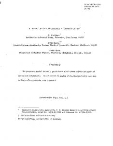
FIG. 1. Comparison of modeled vs HITRAN 2000 line-by-line fractional transmitted radiation. Results are shown for (a)–(h) eight gases, each of which is assumed to be the only absorber for each figure [absorption coefficients from Eq. (7)]. Pathlengths are given in the figures and are 22.22 times the layer pathlengths shown in Table 3, giving pathlengths approximately through the entire atmosphere. Other conditions were T ⫽ 270 K and pa ⫽ 322.15 hPa. For each of the 99 model wavelength intervals (50–148 in Table 1), the product of pathlength and each line-by-line absorption coefficient in the probability interval was summed and applied to a Beer’s law transmission equation to obtain the HITRAN result. For the model, absorption coefficients for 16 probability intervals in each wavelength interval were derived, and transmission was calculated with Beer’s law.

where Ng is the number of absorbing gases, b⬘q,␭,i is the interpolated absorption coefficient, and uq is the current pathlength of gas q. For cases where the number of model probability

intervals is a factor of L smaller than the number of probability intervals in the dataset generated, the gas absorption optical depth in coarser probability interval m (which varies from 1, . . . , Np/L) is calculated with

FEBRUARY 2005

513

JACOBSON

FIG. 1. (Continued)

冋兿

册

Ng

␶a,g,␭,m ⫽ ⫺ln

q⫽1

where Lm

Aq,␭,m ⫽

兺

i⫽L共m⫺1兲⫹1

共10兲

共1⫺Aq,␭,m兲 ,

Wi共1 ⫺ e⫺b⬘q,␭,iuq兲

冒

Lm

兺

i⫽L共m⫺1兲⫹1

Wi. 共11兲

With this method, absorptivities are first calculated in each finer probability interval. They are then weighted by the probability (Wi), and optical depths are extracted from an inverse calculation. Two alternatives to this method are merely to average linearly the absorption coefficients among multiple probability intervals or to generate a table with fewer probability intervals. However, both methods result in excessive absorption relative to Eqs. (10) and (11), as discussed in section 3.

3. Comparison of results with line-by-line data In this section, transmission results from the technique described in section 2 are compared with transmissions from line-by-line data. Figures 1a–1h compare model transmissivities for eight gases through one model layer when each gas is assumed to be the only absorber in the atmosphere, and with absorption coefficients in each wavelength interval calculated from Eq. (7). The model wavelength grid is given in Table 1. Pathlengths are approximately those of the gas through the entire atmosphere. The figure shows relatively high model accuracy for every gas in nearly every wavelength interval. Figure 2 is similar to Fig. 1, except in Fig. 2, 1) the gas absorption coefficient is that of a secondary absorber [Eq. (8)] for all wavelength intervals except those where the gas is specified as a primary absorber in Table 1, 2) gases other than the gas of interest were treated as the primary absorber when specified in Table

1, and 3) the pathlength of each gas in Fig. 2 is 1.5% that in Fig. 1, thus more representative of a typical model layer. In Fig. 2, the model is accurate for all gases in all wavelength intervals where the gas is a primary absorber but slightly underpredicts absorption for some wavelength intervals where the gas is a secondary absorber (e.g., CO2 at 2.8 ␮m, N2O at 4.5 ␮m, CH4 at 3.5 ␮m). In all cases of underabsorption, correct absorption is relatively weak, so the error relative to initial transmission is not large. Figures 3a,b show the transmission through all 11 gases simultaneously and through four (instead of one) layer, each with different temperature and pressure. The only difference in input between Figs. 3a,b is pathlength. The only noticeable error in either figure occurs at around 40–50 ␮m, where absorption is slightly overpredicted. Figure 4 shows transmissions for the conditions in Fig. 3b, except as follows: in Figs. 4a and 4c, the number of probability intervals was compressed from 16 with Eqs. (10) and (11). In Fig. 4b, there were 8 instead of 16 probability intervals used to calculate the original absorption coefficients. A comparison of Fig. 4a with Fig. 3b shows that the use of model Eqs. (10) and (11) to convert 16 probability coefficients to 8 caused a slight increase in error at several wavelength intervals. A comparison of Fig. 4b with Fig. 4a shows that deriving the absorption coefficients with 8 probability intervals from the start caused greater error than compressing 16 to 8 intervals. Figure 4c shows that compressing 16 to 4 intervals with Eqs. (10) and (11) caused an error greater than starting with 8 intervals (Fig. 4b). Figures 3 and 4 were analyzed for integrated transmission errors, calculated as

E⫽

1 N␭

N␭

model line |Im ⫺I m | 1 ⫽ I N␭ 0 m⫽1

兺

N␭

兺 |T

model line ⫺T m |, m

m⫽1

共12兲

514

JOURNAL OF THE ATMOSPHERIC SCIENCES

VOLUME 62

FIG. 2. (a)–(g) Same as Fig. 1, except that each panel here shows the transmission for the given gas when the gas shown is a secondary absorber [with absorption coefficients from Eq. (8)] in each wavelength interval unless identified as a primary absorber for the wavelength interval in Table 1. The pathlength of each gas is one-third the layer pathlength given in Table 3. (h)–(j) Three additional gases (those with cross-sectional data), not shown in Fig. 1.

where N␭ ⫽ 99 is the number of wavelength intervals; ⫽ I model /I0 is the model-predicted transmissivity T model m m through 11 gases and two layers in model wavelength ⫽ I line interval m; T line m m /I0 is the integrated line-byline transmissivity; I0 is incident irradiance; and I is transmitted irradiance. The errors for Figs. 3a and 3b

were 0.0065 and 0.0054, respectively. The errors for Figs. 4a–c were 0.0081, 0.015, and 0.023, respectively. Thus, for the cases where 16 probability intervals were used (Figs. 3a,b), the error was ⬍0.7%. For the case where 8 probability intervals were compressed from 16 (Fig. 4a), the error was ⬍1%. When 8 prob-

FEBRUARY 2005

JACOBSON

515

FIG. 2. (Continued)

ability intervals were used to derive the coefficients (Fig. 4b) or when 4 intervals were compressed from 16 (Fig. 4c), the error was ⬎1%. Although these transmission errors are small, they may lead, in some cases, to higher errors in heating rates when the absorption is small. Errors can be minimized by not compressing probability intervals and/or increasing the number of probability intervals at the expense of more computer time. Finally, a global 3D simulation was run with GATOR-GCMOM with the wavelength grid shown in Fig. 1 and with 16 probability intervals compressed to 8 using Eqs. (10) and (11) to ensure accuracy ⬍1%. For the calculations, wavelength intervals 1–86 (0.165–0.805 ␮m) in Table 1 were confined to one probability interval, and wavelength intervals 87–148 (0.805–1000 ␮m) were broken into 8 probability intervals each. A total of 694 radiative transfer calculations were performed in each model column for each cloudy and clear-sky conditions [86 wavelengths ⫻ 1 probability interval each, 62 (solar ⫹ thermal IR) ⫹ 14 (overlap) wavelengths ⫻ 8 probability intervals each] with the radiative transfer algorithm of Toon et al. (1989). The model was set up over a 4°S–N ⫻ 5°W–E global grid, with 39 sigma-

pressure layers from the ground to 0.425 hPa (⬇55 km), including 23 tropospheric layers and 4 layers below 1.3 km. The model was run for 1 yr. Figure 5 compares the yearly and zonally averaged top-of-the-atmosphere (TOA) thermal-IR irradiance from the model with satellite-derived data. The model predicted the data well at all latitudes, except for some difference in the 10°– 25°N band.

4. Conclusions A “multiple-absorber” correlated-k distribution method that uses spectral-mapping techniques was developed that parameterizes line-by-line data among multiple-absorbing gases for use in three-dimensional atmospheric models. The method ensures exact correlation of absorption frequencies for all gases within each probability interval of each wavelength interval and for all altitudes. A technique was also developed to compress the number of probability intervals in an atmospheric model more accurately than merely reducing the number of intervals during the

516

JOURNAL OF THE ATMOSPHERIC SCIENCES

VOLUME 62

FIG. 3. (a) Same as Fig. 1, but for transmission simultaneously through all 11 gases and four layers of the atmosphere (T ⫽ 210 K, pa ⫽ 0.3611 hPa for layer 1; T ⫽ 250 K, pa ⫽ 22.57 hPa for layer 2; T ⫽ 270 K, pa ⫽ 322.15 hPa for layer 3; T ⫽ 310 K, pa ⫽ 1050.0 hPa for layer 4). The pathlength of each gas in the first layer was one-third that in Table 3, and pathlengths in layers 2–4 were each one-half those in Table 3. For the model, Np ⫽ 16 and L ⫽ 1. (b) Same as (a), except that the pathlength of each gas in each layer was one-third that in (a).

development of the absorption-coefficient dataset. The accuracy of the method, in comparison with a line-by-line solution, through 11 gases and multiple layers and integrated over wavelengths 0.4–1000 ␮m

with 16 probability intervals per wavelength interval, was ⬍0.7% of incident radiation. The error was ⬍1% when 8 probability intervals were compressed from 16.

FIG. 4. (a) Same as Fig. 3b, except the 16 probability intervals were converted to 8 probability intervals (thus, Np ⫽ 16 and L ⫽ 2) with Eqs. (10) and (11). (b) Same as (a), except only 8 probability intervals were used to derive absorption coefficients in the first place (Np ⫽ 8 and L ⫽ 1). (c) Same as (a), except the 16 probability intervals were converted to 4 probability intervals with Eqs. (10) and (11) (Np ⫽ 16 and L ⫽ 4).

FEBRUARY 2005

JACOBSON

FIG. 5. Comparison of zonally and 1-yr-averaged outgoing thermal-IR irradiance from GATOR-GCMOM with Earth Radiation Budget Experiment data (Kiehl et al. 1998).

Acknowledgments. This work was supported by the NASA Atmospheric Chemistry and Analysis Program and Office of Earth Science, the Environmental Protection Agency Office of Air Quality Planning and Standards, the National Science Foundation Atmospheric Chemistry Division (ATM 0101596), and the Stanford University Global Climate and Energy Project. REFERENCES Ambartzumiam, V., 1936: The effect of the absorption lines on the radiative equilibrium of the outer layers of the stars. Publ. Obs. Astron. Univ. Leningrad, 6, 7–18. Arking, A. A., and K. Grossman, 1972: The influence of line shape and band structure on temperatures in planetary atmospheres. J. Atmos. Sci., 29, 937–949. Fu, Q., and K. N. Liou, 1992: On the correlated k-distribution method for radiative transfer in nonhomogeneous atmospheres. J. Atmos. Sci., 49, 2139–2156. Goody, R. M., R. West, L. Chen, and D. Crisp, 1989: The correlated-k method for radiation calculations in nonhomogeneous atmospheres. J. Quant. Spectrosc. Radiat. Transfer, 42, 539–550. Jacobson, M. Z., 1997: Development and application of a new air pollution modeling system. Part III: Aerosol-phase simulations. Atmos. Environ., 31A, 587–608. ——, 2001: GATOR-GCMM: A global-through urban-scale air pollution and weather forecast model. 1. Model design and treatment of subgrid soil, vegetation, roads, rooftops, water, sea ice, and snow. J. Geophys. Res., 106, 5385–5402. ——, 2002a: Control of fossil-fuel particulate black carbon plus organic matter, possibly the most effective method of slowing global warming. J. Geophys. Res., 107, 4410, doi:10.1029/ 2001JD001376.

517

——, 2002b: Analysis of aerosol interactions with numerical techniques for solving coagulation, nucleation, condensation, dissolution, and reversible chemistry among multiple size distributions. J. Geophys. Res., 107, 4366, doi:10.1029/ 2001JD002044. ——, 2003: Development of mixed-phase clouds from multiple aerosol size distributions and the effect of the clouds on aerosol removal. J. Geophys. Res., 108, 4245, doi:10.1029/ 2002JD002691. Kiehl, J. T., J. J. Hack, and J. W. Hurrell, 1998: The energy budget of the NCAR Community Climate Model: CCM3. J. Climate, 11, 1151–1178. Kondratyev, K. Ya., 1969: Radiation in the Atmosphere. Academic Press, 912 pp. Lacis, A. A., and J. E. Hansen, 1974: A parameterization for the absorption of solar radiation in the earth’s atmosphere. J. Atmos. Sci., 31, 118–133. ——, and V. Oinas, 1991: A description of the correlated k distribution method for modeling nongray gaseous absorption, thermal emission, and multiple scattering in vertically inhomogeneous atmospheres. J. Geophys. Res., 96, 9027–9063. ——, W. C. Wang, and J. Hansen, 1979: Correlated k-distribution method for radiative transfer in climate models: Application to effect of cirrus clouds on climate. NASA Conf. Publ. 2076, 309–314. Liou, K. N., 2002: An Introduction to Atmospheric Radiation. Academic Press, 583 pp. Press, W. H., B. P. Flannery, S. A. Teukolsky, and W. T. Vetterling, 1992: Numerical Recipes: The Art of Scientific Computing. Cambridge University Press, 963 pp. Querry, M. R., 1987: Optical constants of minerals and other materials from the millimeter to the ultraviolet. CRDEC-CR88009, Aberdeen Proving Ground, MD, 331 pp. Rothman, L. S., and Coauthors, 2003: The HITRAN molecular spectroscopic database: Edition of 2000 including updates through 2001. J. Quant. Spectrosc. Radiat. Transfer, 82, doi:10.1016/S0022-4073(03)00146-8. Sander, S. P., and Coauthors, 2000: Chemical kinetics and photochemical data for use in stratospheric modeling. Supplement to Evaluation 12, JPL Publication 00-3, Jet Propulsion Laboratory, 74 pp. Stam, D. M., J. F. de Haan, J. W. Hovenier, and P. Stammes, 2000: A fast method for simulating observations of polarized light emerging from the atmosphere applied to the oxygen-A band. J. Quant. Spectrosc. Radiat. Transfer, 64, 131–149. Toon, O. B., C. P. McKay, T. P. Ackerman, and K. Santhanam, 1989: Rapid calculation of radiative heating rates and photodissociation rates in inhomogeneous multiple scattering atmospheres. J. Geophys. Res., 94, 16 287–16 301. Warren, S. G., 1984: Optical constants of ice from ultraviolet to the microwave. Appl. Opt., 23, 1206–1225. West, R., D. Crisp, and L. Chen, 1990: Mapping transformations for broadband atmospheric radiation calculations. J. Quant. Spectrosc. Radiat. Transfer, 43, 191–199. Yamamoto, G., M. Tanaka, and S. Asano, 1970: Radiative transfer in water clouds in the infrared region. J. Atmos. Sci., 27, 282–292.