Steunpunt Verkeersveiligheid
A Regression Model with ARIMA Errors to Investigate the Frequency and Severity of Road Traffic Accidents
Filip Van den Bossche, Geert Wets, Tom Brijs
PROMOTOR ► ONDERZOEKSLIJN ► ONDERZOEKSGROEP ► RAPPORTNUMMER ►
T F E I
► ► ► ►
Prof. dr. Geert Wets
Kennis Verkeersonveiligheid LUC, PHL, VUB, Vito RA-2004-35
UNIVERSITAIRE CAMPUS GEBOUW D B 3590 DIEPENBEEK 011 26 81 90 011 26 87 11
[email protected] www.steunpuntverkeersveiligheid.be
A Regression Model with ARIMA Errors to Investigate the Frequency and Severity of Road Traffic Accidents
RA-2004-35
Filip Van den Bossche, Geert Wets, Tom Brijs Onderzoekslijn Kennis Verkeersonveiligheid
DIEPENBEEK, 2004. STEUNPUNT VERKEERSVEILIGHEID
Documentbeschrijving Rapportnummer:
R-00-2002-01
Titel:
A Regression Model with ARIMA Errors to Investigate the Frequency and Severity of Road Traffic Accidents
Ondertitel: Auteur(s):
Filip Van den Bossche, Geert Wets, Tom Brijs
Promotor:
Prof. dr. Geert Wets
Onderzoekslijn:
Kennis Verkeersonveiligheid
Partner:
Limburgs Universitair Centrum
Aantal pagina’s:
23
Trefwoorden:
Time series, ARIMA regression models, traffic safety
Projectnummer Steunpunt:
1.3
Projectinhoud:
Analyse van de verkeersveiligheid
Uitgave: Steunpunt Verkeersveiligheid, mei 2004.
Steunpunt Verkeersveiligheid bij Stijgende Mobiliteit Universitaire Campus Gebouw D B 3590 Diepenbeek T 011 26 81 90 F 011 26 87 11 E
[email protected] I www.steunpuntverkeersveiligheid.be
impact
van
mobiliteit
op
de
Samenvatting In dit rapport worden modellen voorgesteld die kunnen gebruikt worden om de frequentie en de ernst van ongevallen in België te verklaren en te voorspellen. Het doel van de studie is de uitbreiding van de kennis over de ontwikkelingen in verkeersveiligheid, en dit door het in kaart brengen van de impact van verschillende verklarende factoren. Meer specifiek wordt nagegaan of het aantal ongevallen en slachtoffers beïnvloed wordt door het weer, de economische toestand en de wetgeving. Belgische maandelijkse gegevens van januari 1974 tot december 1999 werden gebruikt om het model op stellen. Het model werd gebruikt om 12 voorspellingen te maken van de frequentie en de ernst van ongevallen voor het jaar 2000. Met behulp van een regressiemodel met ARIMA foutenterm wordt de impact van verschillende verklarende variabelen op de geaggregeerde verkeersveiligheid gekwantificeerd. Tegelijk wordt de invloed van niet gekende factoren opgevangen door de structuur in de foutenterm. De resultaten tonen een significant effect van het klimaat en de wetgeving, maar de impact van de economische condities blijkt statistisch verwaarloosbaar. Het model leent zich uitstekend voor de voorspelling van de verkeersveiligheid, zoals blijkt uit de vrij goede fit die werd bekomen op een 95% significantieniveau.
Steunpunt Verkeersveiligheid
3
RA-2004-35
Summary In this paper, models are developed to explain and forecast the frequency and severity of accidents in Belgium. The objective of this study is to enhance the understanding of the developments in road safety by studying the impact of various explanatory variables on traffic safety. It is investigated whether the number of accidents and victims is influenced by weather conditions, economic conditions and policy regulations. The model is used to predict the frequency and severity of accidents for a 12-months out-of-sample data set. Monthly Belgian data from January 1974 to December 1999 are used in the model, and predictions are made for the year 2000. Using a regression model with ARIMA errors, the impact of variables on aggregate traffic safety is quantified and at the same time the influence of unknown factors is captured by the error term. The results show a significant effect of weather conditions and laws and regulations on traffic safety, but there seems to be negligible statistical impact of economic conditions. The model can easily be used to forecast traffic safety, as can be seen from the reasonably good fit obtained on a 95% confidence level.
Steunpunt Verkeersveiligheid
5
RA-2004-35
Table of Contents
1. 2. 3.
INTRODUCTION ......................................................................... 7 BACKGROUND .......................................................................... 8 DATA .................................................................................... 9
3.1
Laws and regulations
9
3.2
Weather conditions
9
3.3
Economic conditions
9
3.4
Correction variables
10
4.
METHODOLOGY ........................................................................11
4.1
Multiple Regression
11
4.2
ARIMA Modeling
12
4.3
Regression with ARIMA errors
13
4.4
Forecasting
13
5.
RESULTS ...............................................................................14
5.1
Explanatory model
14
5.1.1
Laws and Regulations .................................................................. 14
5.1.2
Weather Conditions ..................................................................... 16
5.1.3
Economic Conditions .................................................................... 17
5.1.4
Correction Variables..................................................................... 17
5.2
Error model
17
5.3
Forecasting
18
6. 7.
CONCLUSIONS AND FURTHER RESEARCH ...........................................19 REFERENCES ...........................................................................20
Steunpunt Verkeersveiligheid
6
RA-2004-35
1.
INTRODUCTION
For many years, traffic growth and the increasing importance of efficient road transportation led to a large number of road accidents, associated with economic losses and human suffering. Road traffic safety is an important social issue. In Belgium, traffic safety and mobility are main issues on today’s political agenda. Traffic accidents are the combined result of various influences at a certain location and time. In an OECD report (1), some broad categories of factors influencing traffic accident counts are listed. First, the number of accidents depends on some autonomous factors that cannot be influenced on a short-term and countrywide level (weather and state of technology belong to this category). Second, economic conditions like unemployment and income are part of the general climate in which accidents occur. Although these issues are sometimes subjected to political intervention, they are rarely oriented towards road safety improvement. A third category covers the size and the structure of the transportation sector, which is often closely related to exposure (infrastructure, Vehicle Park…). Fourth, the accident countermeasures, formalized in laws and regulations, are explicitly brought into being to reduce the risk of road accidents. Fifth, the accident counts also depend on the data collection system. Changes in collection strategies may produce fictitious increases or decreases in accident counts. A last influence is the random variation in accident counts. Since accidents are, by definition, unwanted events, they cannot be fully predicted. Therefore, part of this phenomenon will always be inexplicable. Although it is intuitively appealing to assume that these factors have an influence on the number of accidents, it would be instructive to get a confirmation of this influence. Given the large number of possible factors, it is not easy to get a clear view on the reasons for the trends in traffic safety. Because of the randomness involved in accident occurrence, the investigation of influential factors should be stochastic in nature. Econometric explanatory models provide a means to test the impact of influential factors. The factors summarized above can be combined in an explanatory model and tested for their (positive or negative) contribution to traffic safety. This makes the models quite appealing to practitioners, who are typically interested in actively increasing the level of traffic safety. The objective of this study is twofold. First, the insights in the developments in road safety are enhanced by studying the complex influence of other, possibly related, variables. More specifically, it is investigated how weather conditions, economic growth and policy regulation may influence the number of accidents and victims. A multiple regression model with ARIMA (Auto-Regressive Moving Average) errors is used to quantify the impact of these factors on aggregate traffic safety. This combination of a regression model and a time series analysis technique allows to build a model with desirable statistical properties, and thus to minimize the risk of erroneous model interpretation. Monthly Belgian data are used for a period from January 1974 to December 1999. Second, an attempt is made to forecast the frequency and severity of accidents for a 12 months out-of-sample data set. In comparison with other studies, results are on both the accident and the victim level and the full possibilities of ARIMA corrections in the errors are used. Also, the impact of exposure is not explicitly tested. Exposure data were not available, and it would be instructive to know how well the models might perform without it. Formal changes in the data collection and reporting system did not occur in the given time period, and therefore were not explicitly modelled. However, some extreme values will be taken into account. The effects of changes in technology are assumed to be absorbed by the structured error term. This text is organized as follows. First, some background information is given on the research done with the kind of models used in the paper. Then, an overview of the data is given. Next, the main ideas of regression with ARIMA errors are discussed. In the results section, the model outcomes and the forecasts are presented and discussed. Also some general conclusions and topics for model improvement and further research are provided.
Steunpunt Verkeersveiligheid
7
RA-2004-35
2.
BACKGROUND
Econometric models (like regression and time series models) appear to be very useful to enhance the understanding of trends in traffic safety. In the OECD report (1), the importance of this kind of models in traffic safety has been extensively described. The wide arsenal of econometric modeling techniques can be very effective in taking into account various influences on aggregate accident figures. This approach is especially useful when many factors are to be tested. Moreover, since accidents are unwanted events, controlled (or “designed”) experiments cannot be used. Accidents are, by definition, non-experimental. Because of the random character, a probabilistic view on the accident process is quite natural. The importance of the use of time series analysis in traffic safety research appears from the attention it deserves in international literature. For some time now, authors have analyzed aspects of traffic safety using (a combination of) regression techniques and time series models. The main ideas of traffic safety development and time series models are described in the COST329 report of the European Commission (2). Apart from the pure ARIMA modeling approach, the document describes the explanatory models, in which traffic safety outcomes are related to a set of explanatory factors. Models with aggregated explanatory variables like population, unemployment or inflation, often referred to as “macro models”, are frequently used in literature to investigate various aspects of traffic safety. An overview of these models is given in Hakim et al. (3). Atkins (4) used intervention analysis to determine the influence of compulsory car insurance, company strikes and a change in the policies of insurance companies on the number of traffic accidents on freeways in British Columbia. Harvey and Durbin (5) studied the effect of seat belt legislation on road casualty rates by means of structural time series modeling. In Fridstrøm et al. (6), Generalized Poisson regression models are used to study the impact of a wide range of explanatory factors on personal injury road accidents and their severity. Fridstrøm et al. (7) investigated the impact of exposure, weather, daylight, reporting routines, speed limits and randomness on the variation in accident counts. Johansson (8) tested the effect of a lowered speed limit on the number of accidents on Swedish motorways, using extended Poisson and Negative Binomial count data models. They incorporate a large number of explanatory factors in a structural time series model. Ledolter et al. (9) investigated the effect of a change in the speed limit on the rural interstate highway system to 65 miles per hour in Iowa. One special class of explanatory models is known as the DRAG family. The DRAG models are structural explanatory models, including a relatively large number of explanatory variables, whose effects on the exposure, the frequency and the severity of accidents are estimated by econometric methods (2). These models are described in Gaudry et al. (10). An overview of macro-economic models and DRAG models can be found in Van den Bossche and Wets (11). This report is an extended version of the report RA-2003-21 (“A Structural Road Accident Model for Belgium”). In comparison with this first version, some major revisions have been implemented. First, an extended dataset is constructed. Instead of working with data from 1986 to 2000, the first observations are now from 1974. Second, the correction structure in the error terms is not limited to AR components only, but allows a full ARIMA structure to model remaining error patterns. Third, some variables that turned out not to be useful were left out of the analysis and non-significant variables were dropped from the final models. The technical background on model construction, however, is still valid. Many technical details on multicollinearity and heteroscedasticity that were previously described are also used in this report.
Steunpunt Verkeersveiligheid
8
RA-2004-35
3.
DATA
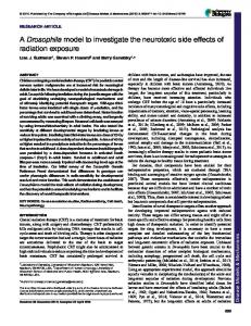
A database has been created for Belgium with explanatory variables on weather, laws and regulations, and economic conditions. Monthly data is used from January 1974 up to December 2000. The last year is used for forecasting purposes. The main part of the data has been gathered from governmental ministries and official documents published by the Belgian National Institute for Statistics. Four dependent variables will be modeled: the number of accidents with lightly injured persons (NACCLI), the number of accidents with persons killed or seriously injured (NACCKSI), the number of persons lightly injured (NPERLI) and the number of persons killed or seriously injured (NPERKSI). The evolution in time of these variables is shown in the first column of Figure 1. The variables NACCKSI and NPERKSI show a decreasing trend. This is less pronounced for NACCLI and NPERLI. All dependent variables show a recurring seasonal pattern, and some months show extremely low observations. The logarithm of the dependent variables will be modeled, written respectively as LNACCLI, LNACCKSI, LNPERLI and LNPERKSI. The independent variables are summarized below.
3.1
Laws and regulations
Five dummy variables are included in the model to study the effect of laws and regulations that were introduced in Belgium at a certain date within the scope of our analysis. These variables are equal to zero before the introduction and equal to one as from the moment of introduction. In June 1975, mandatory seat belt use in the front seats was introduced (LAW0675). The regulations of November 1988 include the introduction of zones with a reduced speed limit of 30 km/h (LAW1188). In January 1992, the speed limit of 50 km/h in urban areas and 90 km/h at road sections with at least 2 by 2 lanes without a raised shoulder or any other separation of the driving directions were introduced, together with regulations on vehicle load, cycling tourists and speed (LAW0192). Starting from December 1994, the 0.05% maximum alcohol level was imposed and higher fines were written out for a 0.08% or higher alcohol level (LAW1294). In April 1996, some regulations on traffic at zebra crossings were put into practice. If a pedestrian is crossing the street, or has the intention to do so, the car driver should give right of way to the pedestrian (LAW0496).
3.2
Weather conditions
Meteorological variables were gathered by the Belgian Royal Meteorological Institute and published by the National Institute for Statistics. The quantity of precipitation (in mm) was measured as an average for the whole country (QUAPREC). The other variables are measured in the climatologic center in Ukkel (in the center of Belgium). These are the number of sunlight hours (HRSSUN) and the monthly percentage (× 100) of days with frost (PDAYFROST), snow (PDAYSNOW), sunlight (PDAYSUN), precipitation (PDAYPREC) and thunderstorm (PDAYTHUN).
3.3
Economic conditions
Some indicators are used to measure economic climate, namely the percentage inflation (INFLAT), and the (log-transformed) number of unemployed people (LNUNEMP). Additionally, the effect of the (log-transformed) number of car registrations (LNCAR) and the percentage of second hand car registrations (POLDNCAR) is tested.
Steunpunt Verkeersveiligheid
9
RA-2004-35
3.4
Correction variables
As could be seen from the graphs in the first column of Figure 1, the number of accidents or victims was extremely low for some months. Peaks can be seen in January 1979, January 1984, January 1985 and February 1997. Either the number of accidents or victims was indeed extremely low in these months, or there was a registration problem. As will be seen further in the text, extreme values disturb the desired properties of the model error terms and should be corrected. Therefore, dummy variables are added to the model. These variables, named JAN79, JAN84, JAN85 and FEB97, are equal to one in the month they represent, and equal to zero elsewhere.
Dependent variables (model data)
Predictions (full line), observed values (dots) and 95% confidence intervals (dotted lines)
Number of accidents with persons lightly injured (NACCLI) January 1974 - December 1999
Number of accidents with persons lightly injured (NACCLI) Predictions for January 2000 - December 2000
5500
5500
4500
4500
3500
3500
2500
2500
1500
1500
jan/74
jan/77
jan/80
jan/83
jan/86
jan/89
jan/92
jan/95
jan/98
Jan
Feb
Mrt
Apr
May
Jun
Jul
Aug
Sep
Oct
MSE(model) = 0.0022
MSE(forecast) = 0.0059
Number of persons lightly injured (NPERLI) January 1974 - December 1999
Number of persons lightly injured (NPERLI) Predictions for January 2000 - December 2000
7500
7500
6500
6500
5500
5500
4500
4500
3500
3500
2500
2500
1500
Nov
Dec
Nov
Dec
1500
jan/74
jan/77
jan/80
jan/83
jan/86
jan/89
jan/92
jan/95
jan/98
Jan
Feb
Mrt
Apr
May
Jun
Jul
Aug
Sep
Oct
MSE(model) = 0.0026
MSE(forecast) = 0.0062
Number of accidents with persons killed or seriously injured (NACCKSI) January 1974 - December 1999
Number of accidents with persons killed or seriously injured (NACCKSI) Predictions for January 2000 - December 2000
2000
1100
1750
1000
1500
900
1250
800
1000
700
750
600
500 jan/74
500 jan/77
jan/80
jan/83
jan/86
jan/89
jan/92
jan/95
jan/98
Jan
Mrt
Apr
May
Jun
Jul
Aug
Sep
Oct
MSE(model) = 0.0030
MSE(forecast) = 0.0046
Number of persons killed or seriously injured (NPERKSI) January 1974 - December 1999
Number of per s ons killed or s er ious ly injur ed (NP ERKSI)
Nov
Dec
Nov
Dec
P r edictions f or J anuar y 2000 - December 2000
2500 2250 2000 1750 1500 1250 1000 750 500 jan/74
Feb
1300 1200 1100 1000 900 800 700 600 500
jan/77
jan/80
jan/83
jan/86
jan/89
jan/92
jan/95
jan/98
J an
MSE(model) = 0.0034
Feb
Mr t
Apr
May
J un
J ul
Aug
Sep
Oct
MSE(forecast) = 0.0057
FIGURE 1: Dependent variables (column 1) and predictions (column 2)
Steunpunt Verkeersveiligheid
10
RA-2004-35
4.
METHODOLOGY
In this study, dependent traffic safety variables are expressed in terms of independent explanatory variables. Multiple linear regression can be used to model a relationship between a dependent variable and one or more independent variables. It allows investigating the effect of changes in the various factors on the dependent variable. If the observations are measured over time, the model is called a time series regression. The resulting statistical relationship can be used to predict future values of the target. If one is interested in the explanatory and predictive power of the regression equation, all necessary assumptions should be met. To this end, a regression model with ARIMA errors will be used as a means to analyze traffic accident time series data. The construction of this kind of models is discussed here. For a thorough and comprehensive overview of regression models, the reader is referred to Neter et al. (12). In Makridakis et al. (13), an introduction to time series analysis is given. Regression models with ARIMA errors are described in Pankratz (14).
4.1
Multiple Regression
The multiple regression model can be written as Yt=β0+β1X1,t+β2X2,t+…+βkXk,t+Nt, where Yt is the t-th observation of the dependent variable, and X1,t,…,Xk,t are the corresponding observations of the explanatory variables. The parameters β0,β1,β2,…,βk are fixed but Using classical estimation unknown, and Nt is the unknown random error term. techniques, estimates for the unknown parameters are obtained. If the estimated values for β0,β1,β2,…,βk are given by b0,b1,b2,…,bk, then the dependent variable is estimated as Yest,t=b0+b1X1,t+b2X2,t+…+bkXk,t, and the estimate Nest,t for the error term Nt is calculated as the difference between the observed and predicted value of the dependent variable: Nest,t=Yt−Yest,t. In the theoretical model, several assumptions are made about the explanatory variables and the error term. When these assumptions are satisfied, the estimators are unbiased and have minimum variance among all linear unbiased estimators. Some of the assumptions of the regression model are, however, frequently violated, especially when applied to time series data. First, the model should be checked for multicollinearity. For computational reasons, the explanatory variables X1,t,…,Xk,t may not be (perfectly) correlated. From a practical point of view, the estimated coefficients will be unstable and unreliable if explanatory variables are highly correlated. In the presence of multicollinearity, the effect of a single explanatory variable cannot be isolated, as the regression coefficients are quite uninformative and their confidence intervals very wide. If the purpose of the model is only to predict the dependent variable, multicollinearity is not a real problem. However, if one is interested in the individual estimated coefficients, results should be interpreted with caution, since only imprecise information can be obtained from the regression coefficients. In the study at hand, the impact of explanatory variables on traffic safety variables, as well as future values for the dependent variable are important. Therefore, the model should be checked for collinear relationships. However, one should realize that multicollinearity is an intrinsic property of non-experimental data. Since controlled experiments are impossible in traffic accident studies, a certain degree of multicollinearity should be accepted. Several techniques can be used to assess the level of multicollinearity. In this study, Variance Inflation Factors (15) and Variance Decomposition (16) are used, but these concepts are not discussed here. Neter et al. (12) argue that a maximum Variance Inflation Factor larger than 10 is an indication of influential multicollinearity. In the final data set, they are all smaller than 5. Therefore it assumed that multicollinearity is at an acceptable level. Second, the error terms should be uncorrelated over time. This assumption is likely to be violated in regression with time series data, giving rise to autocorrelation (the error terms being correlated among themselves). The regression coefficients, although still unbiased, become inefficient, and the estimated standard errors are probably wrong,
Steunpunt Verkeersveiligheid
11
RA-2004-35
making the confidence intervals and t-tests or F-tests no longer strictly applicable (12). In a regression with autocorrelated errors, the errors will probably contain information that is not captured by the explanatory variables, and it is necessary to extract this information to finally end up with uncorrelated (“white noise”) residuals. Typically, the Autocorrelation Function (ACF) and the Partial Autocorrelation Function (PACF) are used to detect autocorrelation among residuals (13). Autocorrelation can be taken into account by adding more complex autoregressive (AR) or moving average (MA) structures to the regression equation, as will be explained further in this text. Third, the error terms should be identically (normally) distributed with mean zero and constant variance. Constant variance is called homoscedasticity. Violation of this condition is called heteroscedasticity. In the presence of heteroscedasticity, the estimators will still be unbiased and consistent, but they will no longer be efficient. Also, the estimates of the standard errors of the regression coefficients will be invalid, leading to a wrong impression of the precision of the results in terms of significance and confidence intervals. Several methods exist to detect heteroscedasticity, like the Goldfeld-Quandt test (17) and Engle's ARCH test (18). In time series, constant variance in the regression error terms is often achieved by transforming the data. In this text, log-transformations are used.
4.2
ARIMA Modeling
In the previous section, the multiple regression model was described, together with possible problems that should be taken care of in order to benefit from the desirable properties of the estimators. When regression is applied to time series data, the error terms are often autocorrelated. If they are, ARIMA models can be used to model the information they contain. The resulting model is then a combination of a multiple regression and an ARIMA model in the error terms. This should enable us to obtain more reliable estimates for the effect of the explanatory variables on the dependent variable. The ARIMA modeling approach expresses a variable as a weighted average of its own past values. The model is in most cases a combination of an autoregressive (AR) part and a moving average (MA) part. Suppose a variable Nt is modeled as an autoregressive process, AR(p). Then, Nt can be expressed as a regression in terms of its own passed values: Nt=C+φ1Nt-1+φ2Nt-2+…+φpNt-p+at, where C is a constant term, φi (i = 1, …, p) are the weights for the autoregressive terms and at is a new random term, which is assumed to be normally distributed “white noise”, containing no further information. Using a backshift operator Bi on Nt, defined as BiNt=Nt-i (i=1,2,…), this process can be written as Nt=C+φ1BNt+φ2B2Nt+…+φpBpNt+at, or (1–φ1B–φ2B2–…–φpBp)Nt=C+at. The series Nt can also be expressed in terms of the random errors of its past values, which is then a moving average MA(q) model: Nt=C+at–θ1at-1–θ2at-2–…–θqat-q, where θj (j=1,…,q) are the weights for the moving average terms. Using the backshift operator, this equals Nt=C–θ1Bat–θ2B2at–…–θqBqat+at, or Nt=C+(1–θ1B–θ2B2–…–θqBq)at. In a more general setting, it is possible to include autoregressive and moving average terms in one equation, leading to an ARMA(p, q) model: (1–φ1B–φ2B2–…–φpBp)Nt=C+(1–θ1B–θ2B2–…– θqBq)at, where at is again assumed to be “white noise”. An ARMA model cannot, however, be applied in all circumstances. It is required that the series be stationary. For practical purposes, it is sufficient to have weak stationarity, which means that the data is in equilibrium around the mean and that the variance around the mean remains constant over time (13). If a series is non-stationary because the variance is not constant, it often helps to log-transform the data, as is done in this text. To have a series that is stationary in the mean, differencing is used. Instead of working with the original series, successive changes in the series are modeled. If necessary, the series can be differenced more than once. For example, in order to obtain a stationary series, the data may be differenced once for the period-by-period (monthly) fluctuations (∇Xt=Xt–Xt-1) and once for the seasonal (yearly) fluctuations: ∇12(∇Xt)=∇12(Xt–Xt-1)=(Xt–Xt-1)-(Xt-12–Xt-13)=Xt–Xt-1–Xt-12+Xt-13. When an ARMA model is
Steunpunt Verkeersveiligheid
12
RA-2004-35
built on differenced data, it is called an ARIMA model, where “I” indicates the differencing.
4.3
Regression with ARIMA errors
The ARIMA modeling approach can now be applied to the multiple regression equation to model the information that remains in the error terms. Assume a regression model with one explanatory variable, denoted as Yt=β0+β1X1,t+Nt. Suppose further that the error terms are autocorrelated, and that they can be appropriately described by an ARMA(1,1) process. This model can then be written as: Yt=β0+β1X1,t+Nt, where (1–φ1B)Nt=(1– θ1B)at, and at is assumed to be white noise. Substituting the correction for the error term into the regression equation gives:
Yt = β 0 + β1 X 1,t +
(1 − θ1B ) a . (1 − φ1B ) t
Because of the specific form in the error terms, the classical least squares methods are not appropriate to estimate the parameters of this equation. Instead, the SAS-ARIMA procedure with Maximum Likelihood estimation is used to set up the models. The Likelihood function is maximized using Marquardt’s method via nonlinear least squares estimation (19). If differencing is applied to the errors in a multiple regression, Pankratz (14) shows that all corresponding series (both of the dependent and the explanatory variables) should be differenced. This can be seen from our small regression example. Differencing the error terms twice results in the following expression, with the ARMA(1,1) model now in the differenced error terms:
∇12 ∇Nt =
(1 − θ1B ) a (1 − φ1B ) t
⇔ Nt =
(1 − θ1B ) a t ∇12 ∇(1 − φ1B ) .
Substituting back this expression into the regression equation gives:
Yt = β 0 + β1 X 1, t +
(1 − θ1B ) a t ∇12 ∇(1 − φ1B )
⇔ ∇12 ∇Yt = β 0' + β1∇12 ∇X 1, t +
(1 − θ1B ) a (1 − φ1B ) t
The intercept is now possibly different, but the (theoretical) regression coefficient β1 is not affected by the differencing operation. Its estimated value may differ slightly, since the estimation is done on different (although related) time series.
4.4
Forecasting
Regression models can easily be used for forecasting purposes. After the model has been developed, estimated values for the dependent variable can be obtained. In order to produce forecasts with a regression model with ARIMA errors, the two parts of the equation need to be predicted. First, for the regression part, future values of the explanatory variables should be available. National or regional government institutions often produce forecasts for economic indicators. If these forecasts are not available, the explanatory variables must be estimated. In our models, “future” monthly values for the year 2000 are available for each of the explanatory variables and therefore no estimation is done. Second, in the ARIMA error part, the errors should be replaced by their estimated values. To depict uncertainty in the predicted values, 95% confidence intervals are provided.
Steunpunt Verkeersveiligheid
13
RA-2004-35
5.
RESULTS
In this section, the results of our models will be presented. The models were tested for multicollinearity, based on Variance Inflation Factors (15) and Variance Decomposition (16). The set of variables used to model the number of accidents and their severity had an acceptable level of multicollinearity. Next, the models were tested for heteroscedasticity. It turned out that this was not a serious problem in the models, so that no corrections were needed. For stationarity reasons, the models were developed on the differenced data. It is reasonable to assume that the number of accidents or victims in one period may in some sense be related to the same number in the previous period. Also, since monthly counts are used, a recurring seasonal pattern will be present. Therefore, both period-by-period and yearly differences were taken. Further, the intercept was dropped from the equations. When differencing is done, the intercept may be interpreted as a deterministic trend, which is not always realistic (14). Based on the ACF and the PACF and the corresponding confidence intervals, some AR and MA terms were defined for the error terms of the regression equations. According to the Ljung-Box Q*-statistics (20), the final error terms were accepted to be “white noise”.
5.1
Explanatory model
The next section gives an overview of the results obtained. Models were built for LNACCLI, LNACCKSI, LNPERLI and LNPERKSI. In Table 1, the parameter estimates for the four equations are presented. Only the significant variables were retained (each model was re-estimated after dropping the non-significant variables). For each variable, the parameter estimate and the approximate absolute t-value (between brackets) are reported. If an absolute t-statistic is larger than 2, the explanatory variable has a significant influence on at least a 95% confidence level. If absolute the t-value is larger than 1.64, then the explanatory variable has a significant influence on a confidence level of at least 90%. Lower confidence levels were not retained. Also the Akaike Information Criterion (AIC) and the error standard deviation are reported for the estimated models and for the corresponding pure ARIMA models (without covariates). The AIC is smaller when less parameters are used or when the likelihood increases. The lower the AIC, the better the model is. Furthermore, it is interesting to compare the AIC value with an ARIMA model without explanatory variables. This gives an idea of the model quality improvement when covariates are used. There is an increase in model fit of about 30% for all models when explanatory variables are considered. 5.1.1 Laws and Regulations The results on laws and regulations are very interesting and instructive. The mandatory seat belt use in the front seats (LAW0675) resulted in considerable and highly significant increases in traffic safety. The seat belt law results are in line with many other models in literature. Hakim et al. (3) postulated that seat belt legislation and enforcement generally reduce the number of fatalities and the severity of injuries. Harvey and Durbin (5) and McCarthy (21) found similar results. The introduction of ZONE 30 in urban areas (LAW1188) is not significant. It would be good practice to further investigate this result on a local level, since the law is only valid in some urban areas. The law of January 1992 (LAW0192), which imposes new speed limits, reduces all kinds of accidents and victims. In Fridstrøm et al. (7) the effects of speed reduction on rural roads and freeways from 90 km/h to 80 km/h and from 110 km/h to 100 km/h were both insignificant, as opposed to the urban speed limit reduction from 60 km/h to 50 km/h. Yet another promising effect can be noted for the laws and fines on alcohol (LAW1294). This law seems to be very useful in reducing LNACCKSI and LNPERKSI. It is, however, less efficient for the lightly injured outcomes LNACCLI and LNPERLI. This underlines the hypothesis that drunken drivers do frequently provoke serious or fatal accidents. In Fournier et al. (22), the combined law on alcohol and speed limits caused a decline in the number of accidents with persons killed and injured. Also in Blum et al. (23), alcohol limits reduce the
Steunpunt Verkeersveiligheid
14
RA-2004-35
number of accidents. The laws of April 1996 (LAW0496), controlling traffic at zebra crossings, are not significant. These new regulations neither increase nor decrease the number of accidents and victims. Just like for the introduction of ZONE 30 in urban areas (LAW1188), these results should be checked on a more local level. TABLE 1: Results for the four models LNACCLI LNACCKSI LNPERLI LNPERKSI Laws and Regulations -0.0696 -0.1346 -0.1204 -0.1594 LAW0675 (2.40) (3.82) (3.75) (4.24) LAW1188 -0.0706 -0.0624 -0.0635 -0.0755 LAW0192 (2.50) (1.87) (2.03) (2.11) -0.1049 -0.0928 LAW1294 (3.12) (2.57) LAW0496 Weather Conditions 0.0005 0.0005 QUAPREC (4.71) (4.39) 0.0007 0.0007 0.0008 0.0009 PDAYPREC (2.84) (3.34) (2.88) (4.02) -0.0011 -0.0013 -0.0009 -0.0012 PDAYFROST (5.63) (5.77) (4.36) (4.81) PDAYSNOW 0.0006 0.0005 PDAYTHUN (1.93) (2.06) PDAYSUN 0.0005 0.0005 0.0004 0.0005 HRSSUN (5.38) (5.35) (4.17) (4.80) Economic Conditions INFLAT LNUNEMP LNCAR POLDNCAR Correction Variables -0.4409 -0.5736 -0.4581 -0.5498 JAN79 (10.40) (12.05) (9.97) (10.75) -0.4492 JAN84 (9.87) -0.2852 -0.2815 -0.2937 -0.2890 JAN85 (6.80) (5.85) (6.46) (5.62) -0.2181 -0.1282 -0.2377 -0.1243 FEB97 (5.08) (2.66) (5.09) (2.31) Goodness of Fit AIC -949.54 -860.50 -904.17 -821.89 Error St. Dev. 0.0467 0.0547 0.0506 0.0586 Goodness of Fit for an ARIMA model without covariates AIC -713.62 -656.07 -654.54 -651.05 Error St. Dev. 0.0728 0.0805 0.0804 0.0784
Steunpunt Verkeersveiligheid
15
RA-2004-35
It is assumed that the introduction of a law results in a sudden and permanent increase or decrease in the dependent variable. For example, the introduction of the seat belt law resulted in a 1-exp(-0.0696)=6.7% reduction of the number of accidents with lightly injured persons, ceteris paribus. This assumption of a "step-based intervention” is not always a natural one. Moreover, it is not possible to isolate the effect of a single measure when several regulations are put into practice at the same or a nearby moment in time. The significant impact of laws and regulations may be better described as “something changed at that time”, instead of attributing the whole effect to the law itself. Nevertheless it makes sense to test whether these changes are indeed substantial. 5.1.2 Weather Conditions The weather conditions seem to have an impact on traffic safety. First, an extra millimeter of precipitation in a given month (QUAPREC) will increase NPERLI and NACCLI by exp(0.0005)-1=0.05%. However, this variable neither affects LNACCKSI nor LNPERKSI. If the quantity of precipitation is known to be higher in a given period, a lower number of fatal accidents is to be expected, because of more prudent driving behavior. If, however, drivers are surprised by sudden heavy rainfall, fatal accidents and severe injuries are more likely. Probably these two opposite powers cancel out the effect of quantity of precipitation on the accidents with persons killed and seriously injured and the corresponding number of victims. On the other hand, the percentage number of rainy days (PDAYPREC) has a similar influence on all dependent variables. For example, if PDAYPREC increases by 1 in a given month, then NACCLI will be exp(0.0007)-1=0.07% higher on average. More days with the same kind of (bad) weather may create a sort of habituation, leading to more risky driving behavior. Also, this variable does not take into account the quantity of precipitation, probably resulting in a more general effect. The rainfall increases accident toll also according to other studies, like for example in Fridstrøm et al. (6, 7) and in Tegnér et al. (24). Blum et al. (23) stated that the presence of rain has larger and more general impacts than the amount of rain, which is in line with our findings. The impact of the percentage number of days with thunderstorm (PDAYTHUN) is comparable to that of the quantity of precipitation. A higher number of days with thunderstorm significantly increases LNACCLI and LNPERLI. This may be partly explained by a lower visibility in stormy weather. A higher monthly percentage number of days with frost (PDAYFROST) decreases all dependent variables. Road users seem to compensate for the higher risk imposed by frost. They probably adjust their driving habits more than in normal weather conditions. Another possible explanation is the lower number of kilometres driven (exposure) in winter. Furthermore, winter conditions may induce a more prudent driving behavior. One can also argue, as is done in Fridstrøm et al. (7), that less proficient drivers may avoid driving on slippery roads, thereby increasing the average driving capacity of drivers on the road. Moreover, lower speeds in extreme weather conditions lead to less serious accidents. The variable PDAYSNOW is not significant in our models, almost surely because snow is not common in Belgium. In countries where snow is more prevalent, the effect on traffic safety is comparable to that of frost. For example, Tegnér et al. (24) report a lower number of accidents in extremely cold weather. In Fridstrøm (25), less injury accidents were found when the ground is covered with snow, but accident frequency goes up during days with snowfall, which is in line with our precipitation results. Next, the monthly number of sunny hours (HRSSUN) increases all dependent variables. For example, an increase of HRSSUN by 1 (hour) results in a exp(0.0005)-1=0.05% increase in NACCLI. It is possible that exposure is higher on sunny days, and that drivers are more relaxed and concentrated less than normal. Also it is plausible to assume a higher exposure on sunny days, or accidents caused by the dazzling sun, as was also found in Blum et al. (23). Other climatologic variables like the percentage number of days with snow (PDAYSNOW) and sunlight (PDAYSUN) were not significant.
Steunpunt Verkeersveiligheid
16
RA-2004-35
Given the fact that these variables are often important in other models, it is clear that the effect of weather data is related to the geographic properties of the area of concern. Results may also vary according to the time period considered. A climatologic variable studied on a daily level may provide completely different insights than when studied on a monthly level. Further research on this topic is necessary. 5.1.3 Economic Conditions The effect of economic conditions on traffic safety is far less clear in comparison with the other categories of variables. None of the tested economic indicators was significant in our models. In other models however, results are often significant, although not always unambiguous. In Hakim et al. (3), unemployment and income are said to increase traffic safety, because of a lower ability to travel and a higher demand for safer cars. In contrast, Jaeger et al. (26) found that a rise in unemployment may decrease traffic safety. One of the reasons might be a divergent variable construction. Also different social protection systems may explain dissimilarity between various models. Further, the number of car registrations (LNCAR) and the percentage of second hand car registrations (POLDNCAR) were not significant. In many other models the vehicle fleet has a significant influence on traffic safety. This confirms our impression that these variables are only weak approximations for the size of the vehicle fleet, for which no accurate data could be obtained. Moreover, the effect of economic variables might have disappeared because of the differencing operations in the model. Since transitions in economic variables are sometimes very slow, the effect after differencing may be almost negligible. Hakim et al. (3) conclude that the net effect of economic growth on traffic safety is not clear. There may be a decreasing effect from an increase in exposure and an increasing effect from demand and supply of safety. These opposite effects may nullify each other, obscuring the different parts in the relationship. 5.1.4 Correction Variables The correction variables, introduced to account for deviating behavior of the series, are highly significant. For LNACCLI, the number of accidents was 1-exp(-0.4409)=36% lower on average in JAN79. The deviations were clearly present in the graphs for the dependent variables and in the residual plots (not shown here), which justifies their inclusion in the models. It is possible that these numbers are not “accidentally” deviating. For example, JAN79 and JAN85 were characterized by extremely cold weather, and FEB97 was one of the least sunny and most rainy months of the century. For JAN84, which is only significant in one equation, no such interpretation could be found, probably indicating a registration error. It is clear from the results that these corrections significantly improve the accordance between the original and the estimated series, although one should be aware of the danger of over-fitting.
5.2
Error model
The error terms of the regression equations should be corrected for possible autocorrelation. As explained in the methodology section, both Autoregressive (AR) and Moving Average (MA) corrections are possible. For LNACCLI, it is found that (1+0.1916B4)Nt=(1–0.7327B)(1–0.8989B12)at. Here, Nt is the original regression error term, while at is the corrected (“white noise”) error term, which contains no further information. The backshift operator B is the same as defined before. For LNPERLI, the In the expression is very similar: (1+0.1527B4)Nt=(1–0.7284B)(1–0.8755B12)at. correction term for LNACCKSI, only moving average terms were needed: Nt=(1– 0.7197B–0.1473B4+0.1408B6)(1–0.2011B10)(1–0.8237B12)at. For LNPERKSI, the error expression is (1+0.1583B4+0.1652B10)Nt=(1–0.7184B)(1–0.8018B12)at. It is not always easy to give a clear-cut interpretation for the error structure models, but the one-by-one and the yearly backshift express the fact that each month carries some
Steunpunt Verkeersveiligheid
17
RA-2004-35
information from the previous month, and from the same month in the previous year, which is no surprise indeed.
5.3
Forecasting
Forecasting is done on the data for the year 2000. If forecasting is done with a regression model, data for the input series (the explanatory variables) should be available. In our case, “future” monthly values for the explanatory variables for 2000 are used. The values for the explanatory variables are not estimated, and are assumed to be known with certainty. The predicted values (full line) and the 95% confidence intervals (dotted lines) are plotted in the second column of Figure 1. To assess the quality of the prediction, also the real numbers of accidents and victims are plotted (dots). Note that the data and the confidence intervals have been transformed back to the original series. The predicted values are quite close to the observed values. Only a few observed values are outside the prediction intervals. To quantify forecast accuracy, the Mean Squared Error (MSE) is reported, which is the average of all squared deviations between the observed and the predicted values (13). This value is calculated separately for the training data, on which the model has been developed, and for the predictions. The latter are not used for model fitting, and are completely new for the model. This explains why the MSE on these data is much higher. It is, however, a better indicator of model quality, because a good model fit does not always imply good forecasting. On the other hand, the graphs show that most of the fluctuations in the series is captured. Also note that accidents are better predicted than victims (shown by a lower MSE value for the predictions).
Steunpunt Verkeersveiligheid
18
RA-2004-35
6.
CONCLUSIONS
AND
FURTHER RESEARCH
In this study, regression models with ARIMA errors were developed to investigate the impact of weather, laws and regulations and economic conditions on the frequency and severity of accidents in Belgium. If all statistical assumptions are fulfilled, the combination of regression and time series analysis offers a powerful means to investigate the impact of various factors on traffic safety. The results show that weather conditions and some policy regulations have a significant influence on traffic safety. The impact of the economic conditions is not significant. The models were subsequently used to make out-of-sample forecasts for the dependent variables. The predictions were plausible and quite accurate, but nevertheless they show the intrinsic volatility present in traffic safety outcomes. This underlines the importance of a statistical approach to accident analysis. The models developed in this text show large potential for describing the long-term trends in traffic safety. On the one hand, they can isolate the effect of phenomena that cannot be influenced, but that certainly act upon traffic safety, like weather conditions. Similarly, macro-economic indicators and socio-demographic evolutions could be added to the model. On the other hand, the efficiency of laws and regulations or time-specific interventions can be tested. These are the direct tools for increasing the level of traffic safety. This looks appealing to practitioners, who may find it useful to know what factors other than policy regulations are influencing traffic safety. However, some aspects should be given more attention. Regression models with ARIMA errors could become quite complex. It is important to look for the most parsimonious model. As regards the data, it is clear that the number of variables tested in our models is limited. It would be interesting to test also other factors like exposure, demography, active and passive car safety, speed, observed seat belt use and alcohol consumption. Nevertheless, the combination of a regression model and an ARIMA error structure gives an acceptable fit, even without these elements. The effects of omitted factors, although not explicitly tested, are reflected in the error terms. Also, adding explanatory variables brings more multicollinearity into the model and requires a higher number of observations. Extending the model with more factors may result in a better understanding of the complex influences on traffic safety, but model building will become more complex. The elaboration of data quality and availability, together with the development of extensive but statistically sound models should lead to high quality results that can be used as a guide to more directed analyses. These are important topics for further research.
Steunpunt Verkeersveiligheid
19
RA-2004-35
7.
REFERENCES
(1)
OECD Road Transport Research. Road Safety Principles and Models: Review of Descriptive, Predictive, Risk and Accident Consequence Models. OCDE/GD(97)153, Organisation for Economic Co-operation and Development, Paris, 1997.
(2)
COST329: Models for Traffic and Safety Development and Interventions. Final Report of the Action, Directorate General for Transport, European Commission, 1999.
(3)
Hakim, S., Shefer, D. and Hakkert, A.S. A Critical Review of Macro Models for Road Accidents. Accident Analysis and Prevention, 23, 5, 1991, pp. 379-400.
(4)
Atkins, S.M. Case study on the use of intervention analysis applied to traffic accidents. Journal of the Operations Research Society, 30, No. 7, 1979, pp. 651659.
(5)
Harvey, A.C. and Durbin, J. The effect of seat belt legislation on British road casualties: a case study in structural time series modeling. Royal Statistical Society, Journal (A), 149, Part 3, pp. 187-227.
(6)
Fridstrøm, L. and Ingebrigtsen, S. An aggregate accident model based on pooled, regional time-series data. Accident Analysis and Prevention, Vol. 23, 1991, pp. 363378.
(7)
Fridstrøm, L., Ifver, J., Ingebrigtsen, S., Kulmala, R. and Thomsen, L.K. Measuring the contribution of randomness, exposure, weather and daylight to the variation in road accident counts. Accident Analysis and Prevention, Vol. 27, 1995, pp. 1-20.
(8)
Johansson, P. Speed limitation and motorway casualties: a time series count data regression approach. Accident Analysis and Prevention, Vol. 28, 1996, pp. 73-87.
(9)
Ledolter, J. and Chan, K.S. Evaluating the impact of the 65 mph maximum speed limit on Iowa rural interstates. American Statistician, 50, 1996, pp. 79-85.
(10) Gaudry, M. and Lassarre, S. Structural Road Accident Models: The International DRAG Family. Elsevier Science, Oxford, 2000. (11) Van den Bossche, F. and Wets, G. Macro Models in Traffic Safety and the DRAG Family: Literature Review. Report RA-2003-08, Flemish Research Center for Traffic Safety, Diepenbeek, 2003. (12) Neter, J., Kutner, M. H., Nachtsheim, C. J. and Wasserman, W. Applied Linear Statistical Models. WCB/McGraw-Hill, 1996. (13) Makridakis, S., Wheelwright, S. and Hyndman, R. Forecasting: Methods and Applications. Third edition, John Wiley and Sons, 1998. (14) Pankratz, A. Forecasting With Dynamic Regression Models. John Wiley & Sons, 1991. (15) Marquardt D.W. Generalized inverses, ridge regression, biased linear estimation and non-linear estimation. Technometrics, 12, 1970, pp. 591-612. (16) Belsley D.A., Kuh E. and Welsh R.E. Regression diagnostics: identifying influential data and sources of collinearity. John Wiley and Sons, New York, 1980.
Steunpunt Verkeersveiligheid
20
RA-2004-35
(17) Goldfeld, S.M. and Quandt, R.E. Some Tests for Homoskedasticity. Journal of the American Statistical Association, 60, 1965, pp. 539-547. (18) Engle, R. Autoregressive Conditional Heteroskedasticity with Estimates of the Variance of United Kingdom Inflation. Econometrica, Vol. 50, 1982, pp. 987-1007. (19) SAS Institute Inc. SAS OnlineDocTM, Version 7-1, 1999. (20) Ljung, G. and Box, G. On a Measure of Lack of Fit in Time Series Models. Biometrika, 67, 1978, pp. 297-303. (21) McCarthy, P. The TRACS-CA Model for California. In: Structural Road Accident Models: The International DRAG Family (Gaudry, M. and Lassarre, S. Eds.). Chap. 7, 185-204, Elsevier Science, Oxford, 2000. (22) Fournier, F. and Simard, R. The DRAG-2 Model for Quebec. In: Structural Road Accident Models: The International DRAG Family (Gaudry, M. and Lassarre, S. Eds.). Chap. 2, pp. 37-66, Elsevier Science, Oxford, 2000. (23) Blum, U. and Gaudry, M. The SNUS-2.5 Model for Germany. In: Structural Road Accident Models: The International DRAG Family (Gaudry, M. and Lassarre, S. Eds.). Chap. 3, pp. 67-96, Elsevier Science, Oxford, 2000. (24) Tegnér, G., Holmberg, I., Loncar-Lucassi, V. and Nilsson, C. The DRAG-Stockholm Model. In: Structural Road Accident Models: The International DRAG Family (Gaudry, M. and Lassarre, S. Eds.). Chap. 5, pp. 127-156, Elsevier Science, Oxford, 2000. (25) Fridstrøm, L. The TRULS-1 Model for Norway. In: Structural Road Accident Models: The International DRAG Family (Gaudry, M. and Lassarre, S. Eds.). Chap. 4, pp. 97126, Elsevier Science, Oxford, 2000. (26) Jaeger, L. and Lassarre, S. (2000). The TAG-1 Model for France. In: Structural Road Accident Models: The International DRAG Family (Gaudry, M. and Lassarre, S. Eds.). Chap. 6, pp. 157-184, Elsevier Science, Oxford, 2000.
Steunpunt Verkeersveiligheid
21
RA-2004-35