A Reinforcement Learning Approach - Sound & Music Computing Lab

Exploration in Interactive Personalized Music Recommendation: A Reinforcement Learning Approach XINXI WANG, National University of Singapore YI WANG, Institute of High Performance Computing, A*STAR DAVID HSU and YE WANG, National University of Singapore

Current music recommender systems typically act in a greedy manner by recommending songs with the highest user ratings. Greedy recommendation, however, is suboptimal over the long term: it does not actively gather information on user preferences and fails to recommend novel songs that are potentially interesting. A successful recommender system must balance the needs to explore user preferences and to exploit this information for recommendation. This article presents a new approach to music recommendation by formulating this exploration-exploitation trade-off as a reinforcement learning task. To learn user preferences, it uses a Bayesian model that accounts for both audio content and the novelty of recommendations. A piecewise-linear approximation to the model and a variational inference algorithm help to speed up Bayesian inference. One additional benefit of our approach is a single unified model for both music recommendation and playlist generation. We demonstrate the strong potential of the proposed approach with simulation results and a user study. Categories and Subject Descriptors: H.3.3 [Information Search and Retrieval]: Information Filtering; H.5.5 [Sound and Music Computing]: Modeling, Signal Analysis, Synthesis and Processing General Terms: Algorithms, Experimentation Additional Key Words and Phrases: Recommender systems, machine learning, music, model, application ACM Reference Format: Xinxi Wang, Yi Wang, David Hsu, and Ye Wang. 2014. Exploration in interactive personalized music recommendation: A reinforcement learning approach. ACM Trans. Multimedia Comput. Commun. Appl. 11, 1, Article 7 (August 2014), 22 pages. DOI: http://dx.doi.org/10.1145/2623372

1. INTRODUCTION

A music recommendation system recommends songs from a large database by matching songs with a user’s preferences. An interactive recommender system adapts to the user’s preferences online by incorporating user feedback into recommendations. Each recommendation thus serves two objectives: (i) satisfy the user’s current musical need, and (ii) elicit user feedback in order to improve future recommendations. Current recommender systems typically focus on the first objective while completely ignoring the other. They recommend songs with the highest user ratings. Such a greedy strategy, that does not actively seek user feedback, often results in suboptimal recommendations over the long term. Consider the simple example in Figure 1. The table This research is supported by the Singapore National Research Foundation under its International Research Centre at Singapore Funding Initiative and administered by the IDM Programme Office. Author’s addresses: X. Wang, Department of Computer Science, National University of Singapore, SG, 117417; Y. Wang, Computing Science Department, Institute of High Performance Computing, A*STAR, SG, 138632, Singapore; D. Hsu and Y. Wang (corresponding author), Department of Computer Science, National University of Singapore, SG, 117417; email: [email protected]. Permission to make digital or hard copies of all or part of this work for personal or classroom use is granted without fee provided that copies are not made or distributed for profit or commercial advantage and that copies bear this notice and the full citation on the first page. Copyrights for components of this work owned by others than ACM must be honored. Abstracting with credit is permitted. To copy otherwise, or republish, to post on servers or to redistribute to lists, requires prior specific permission and/or a fee. Request permissions from [email protected]. c 2014 ACM 1551-6857/2014/08-ART7 $15.00 ⃝ DOI: http://dx.doi.org/10.1145/2623372 ACM Trans. Multimedia Comput. Commun. Appl., Vol. 11, No. 1, Article 7, Publication date: August 2014.

7

7:2

X. Wang et al.

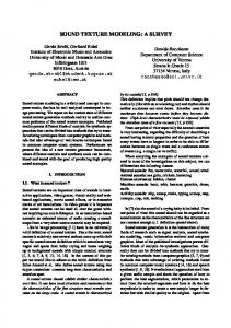
Fig. 1. Uncertainty in recommendation.

contains the ratings for three songs by four users (Figure 1(a)), with 3 being the highest and 1 being the lowest. For simplicity, let us assume that the recommender chooses between two songs B and C only. The target user is 4, whose true ratings for B and C are 1.3 and 1.6, respectively. The true rating is the expected rating of a song by the user. It is a real number, because a user may give the same song different ratings as a result of external factors. In this case, a good recommender should choose C. Since the true user ratings are unknown to the recommender, it may approximate the rating distributions for B and C as Gaussians, PB and PC (Figure 1(b)), respectively, using the data in Figure 1(a). The distribution PB has mean 1.2. The distribution PC has mean 1. PB has much lower variance than PC , because B has more rating data. A greedy recommender (including the highly successful collaborative filtering (CF) approach) would recommend B, the song with the highest mean rating. In response to this recommendation, user 4 gives a rating whose expected value is 1.3. The net effect is that the mean of PB likely shifts towards 1.3 and its variance further reduces (Figure 1(c)). Consequently the greedy recommender is even more convinced that user 4 favors B and will always choose B for all future recommendations. It will never choose C and find out its true rating, resulting in clearly suboptimal performance. To overcome this difficulty, the recommender must take into account uncertainty in the mean ratings. If it considers both the mean and the variance of the rating distribution, the recommendation will change. Consider again Figure 1(b). Although PC has slightly lower mean than PB, it has very high variance. It may be worthwhile to recommend C and gather additional user feedback in order to reduce the variance. User 4’s rating on C has expected value 1.6. Therefore, after one recommendation, the mean of PC will likely shift towards 1.6 (Figure 1(d)). By recommending C several times and gathering user feedback, we will then find out user 4’s true preference C. This example illustrates that a good interactive music recommender system must explore user preferences actively rather than merely exploiting the rating information available. Balancing exploration and exploitation is critical, especially when the system is faced with a cold start, that is, when a new user or a new song appears. Another crucial issue for music recommendation is playlist generation. People often listen to a group of related songs together and may repeat the same song multiple times. This is unique to music recommendation and rarely occurs in other recommendation domains such as newspaper articles or movies. A playlist is a group of songs arranged in a suitable order. The songs in a playlist have strong interdependencies. For example, ACM Trans. Multimedia Comput. Commun. Appl., Vol. 11, No. 1, Article 7, Publication date: August 2014.

Exploration in Interactive Personalized Music Recommendation

7:3

they share the same genre [Chen et al. 2012] or have a consistent mood [Logan 2002], but are diversified at the same time [Zhang et al. 2012]. They may repeat, but are not repetitive. Existing recommender systems based on CF or audio content analysis typically recommend one song at a time and do not consider their interdependencies during the recommendation process. They divide playlist generation into two distinct steps [Chen et al. 2012]: first, choose a set of favored songs through CF or content analysis; next, arrange the songs into a suitable order in a process called automatic playlist generation (APG). In this work, we formulate interactive, personalized music recommendation as a reinforcement learning task called the multi-armed bandit [Sutton and Barto 1998] and address both the exploration-exploitation trade-off and playlist generation with a single unified model. —Our bandit approach systematically balances exploration and exploitation, a central issue well studied in reinforcement learning. Experimental results show that our recommender system mitigates the difficulty of cold start and improves recommendation performance compared to the greedy approach. —We build a single rating model that captures both the user preference over audio content and the novelty of recommendations. It seamlessly integrates music recommendation and playlist generation. —We also present an approximation to the rating model and new probabilistic inference algorithms in order to achieve real-time recommendation performance. —Although our approach is designed specifically for music recommendation, it is possible to generalize it to other media types as well. In the following, Section 2 describes related work. Section 3 formulates the rating model and our multi-armed bandit approach to music recommendation. Section 4 presents the approximate Bayesian models and inference algorithms. Section 5 presents evaluation of our models and algorithms. Section 6 discusses the possible generalization directions of the approach to other media types. Section 7 summarizes the main results and provides directions for future research. 2. RELATED WORK 2.1. Music Recommendation

Since Song et al. [2012] and Shen et al. [2013] provide a very recent and comprehensive review of existing related works on music recommendation, we will first briefly summarize the state-of-the-art and discuss highly relevant work in detail later. Currently, music recommender systems can be classified according to their methodologies into four categories: collaborative filtering (CF), content-based methods, context-based methods, and hybrid methods. Collaborative filtering recommends songs by considering those preferred by other like-minded users. The state-of-the-art method for performing CF is matrix factorization [Koren et al. 2009]. Although CF is the most widely used method, it suffers the notorious cold-start problem, as it cannot recommend songs to new users whose preferences are unknown (the new-user problem) or recommend new songs to users (the new-song problem). Unlike CF, content-based methods recommend songs with audio content similar to the user’s preferred songs [Chen and Chen 2001]. The recommendation quality of content-based systems is largely determined by acoustic features, such as timbre and rhythm features [Song et al. 2012]. Content-based systems solve the new-song problem but not the new-user problem. Context-based music recommender systems are increasingly popular. They recommend songs to match various aspects of the user context (e.g., activities, locations, environment, mood, or physiological states) or text context [Wang et al. 2012; Braunhofer et al. 2013; Kaminskas et al. ACM Trans. Multimedia Comput. Commun. Appl., Vol. 11, No. 1, Article 7, Publication date: August 2014.

7:4

X. Wang et al.

2013; Cheng and Shen 2014; Schedl and Schnitzer 2014; Eck et al. 2007; Knees and Schedl 2013]. Hybrid methods combine two or more of the preceding methods [Yoshii et al. 2006]. There is relatively little work combining music recommendation with playlist generation. In Chen et al. [2012], a playlist is modeled as a Markov process whose transition probability models both user preferences and playlist coherence. In Zheleva et al. [2010], a model similar to latent Dirichlet allocation is used to capture user latent taste and mood of songs. In Aizenberg et al. [2012], a new CF model is developed to model playlists in Internet radio stations. While these earlier approaches also combine recommendation with playlist generation, our model differs in three aspects: (1) it is based on audio content while the previous three depend only on usage data; (2) our model is highly efficient, thus allowing easy online updates; (3) our model is crafted and evaluated based on real-life user interaction data as opposed to data crawled from the Web. Zhang et al. [2012] try to recommend using a linear combination of CF results with the results from an existing novelty model that ranks songs by CF before generating the playlists according to novelty. The parameters for the linear combination are manually adjusted. Moreover, they provide only system-level control of novelty while our method provides personalized control. Other work, such as Hu and Ogihara [2011], generates music playlists within a user’s own music library. They assume that the user’s preference is already known and does not need to be inferred. 2.2. Reinforcement Learning

Unlike supervised learning (e.g., classification, regression) that considers only prescribed training data, a reinforcement learning (RL) algorithm actively explores its environment to gather information and exploits the acquired knowledge to make decisions or predictions. The multi-armed bandit is a thoroughly studied reinforcement learning problem. For a bandit (slot machine) with M arms, pulling arm i will result in a random payoff r sampled from an unknown and arm-specific distribution pi . The objective is to maximize the total payoff given a number of trials. The set of arms is A = {1 . . . M}, known to the player; each arm i ∈ A has a probability distribution pi , unknown to the player. The player also knows he has n rounds of pulls. At the l-th round, he can pull an arm Il ∈ A, and receive a random payoff rIl , sampled from the distribution pIl . The objective !n is to wisely choose the n pulls ((I1 , I2 , . . . In) ∈ An) in order to maximize total payoff l=1 rIl . A naive solution to the problem would be to first randomly pull arms to gather information to learn pi (exploration) and then always pull the arm that yields the maximum predicted payoff (exploitation). However, either too much exploration (the learned information is not used much) or too much exploitation (the player lacks information to make accurate predictions) results in a suboptimal total payoff. Thus, balancing exploration and exploitation is the key issue. The multi-armed bandit approach provides a principled solution to this problem. The simplest multi-armed bandit approach, namely ϵ-greedy, chooses the arm with the highest predicted payoff with probability 1 − ϵ or chooses arms uniformly at random with probability ϵ. An approach better than ϵ-greedy is based on a simple and elegant idea called upper confidence bound (UCB) [Auer 2003]. Let Ui be the true expected payoff for arm i, namely, the expectation of pi ; UCB-based algorithms estimate both its expected payoff Uˆ i and a confidence bound ci from past payoffs, so that Ui lies in (Uˆ i − ci , Uˆ i + ci ) with high probability. Intuitively, selecting an arm with large Uˆ i corresponds to exploitation, whereas selecting one with large ci corresponds to exploration. To balance exploration and exploitation, UCB-based algorithms follow the principle of “optimism in the face of uncertainty” and always select the arm that maximizes Uˆ i + ci . ACM Trans. Multimedia Comput. Commun. Appl., Vol. 11, No. 1, Article 7, Publication date: August 2014.

Exploration in Interactive Personalized Music Recommendation

7:5

Bayes-UCB [Kaufmann et al. 2012] is a state-of-the-art Bayesian counterpart of the UCB approach. In Bayes-UCB, the expected payoff Ui is regarded as a random variable and the posterior distribution of Ui given the history payoffs D, denoted as p(Ui |D), is maintained. Moreover, the fixed-level quantile of p(Ui |D) is used to mimic the upper confidence bound. Similar to UCB, every time Bayes-UCB selects that arm with the maximum quantile. UCB-based algorithms require an explicit form of the confidence bound that is difficult to derive in our case, but in Bayes-UCB, the quantiles of the posterior distributions of Ui can be easily obtained using Bayesian inference. We therefore use Bayes-UCB in our work. There are more sophisticated RL methods such as Markov Decision Process (MDP) ´ 2010], which generalizes the bandit problem by assuming that the states of [Szepesvari the system can change following a Markov process. Although MDP can model a broader range of problems than the multi-armed bandit, it requires much more data to train and is often more computationally expensive. 2.3. Reinforcement Learning in Recommender Systems

Previous work has used reinforcement learning to recommend Web pages, travel information, books, news, etc. For example, Joachims et al. [1997] use Q-learning to guide users through Web pages. In Golovin and Rahm [2004], a general framework is proposed for Web recommendation, where user implicit feedback is used to update the system. Zhang and Seo [2001] propose a personalized Web document recommender where each user profile is represented as vector of terms whose weights of the terms are updated based on the temporal difference method using both implicit and explicit feedback. In Srivihok and Sukonmanee [2005], a Q-learning-based travel recommender is proposed, where trips are ranked using a linear function of several attributes including trip duration, price, and country, and the weights are updated according to user feedback. Shani et al. [2005] use an MDP to model the dynamics of user preference in book recommendation, where purchase history is used as the states and the generated profit the payoffs. Similarly, in a Web recommender [Taghipour and Kardan 2008], browsing history is used as the states, and Web content similarity and user behavior are combined as the payoffs. Chen et al. [2013] consider the exploration/exploitation trade-off in the rank aggregation problem, that is, aggregating partial rankings given by many users into a global ranking list. This global ranking list can be used for unpersonalized recommenders but is of very limited use for personalized ones. In the seminal work done by Li et al. [2012], news articles are represented as feature vectors; the click-through rates of articles are treated as the payoffs and assumed a linear function of news feature vectors. A multi-armed bandit model called LinUCB is proposed to learn the weights of the linear function. Our work differs from theirs in two aspects. Fundamentally, music recommendation is different from news recommendation, due to the sequential relationship between songs. Technically, the additional novelty factor of our rating model makes the reward function nonlinear and the confidence bound difficult to obtain. Therefore we need the Bayes-UCB approach and the more sophisticated Bayesian inference algorithms (Section 4). Moreover, we cannot apply the offline evaluation techniques developed in Li et al. [2011] because we assume that ratings change dynamically over time. As a result, we must conduct online evaluation with real human subjects. Although we believe reinforcement learning has great potential in improving music recommendation, it has received relatively little attention and found only limited application. Liu et al. [2009] use MDP to recommend music based on a user’s heart rate to help the user maintain it within the normal range. States are defined as different levels of heart rate and biofeedback is used as payoff. However: (1) parameters of the model are not learned from exploration and thus exploration/exploitation trade-off ACM Trans. Multimedia Comput. Commun. Appl., Vol. 11, No. 1, Article 7, Publication date: August 2014.

7:6

X. Wang et al.

is not needed; (2) the work does not disclose much information about the evaluation of the approach. Chi et al. [2010] use MDP to automatically generate playlists. Both SARSA and Q-learning are used to learn user preferences and states are defined as mood categories of the recent listening history, similar to Shani et al. [2005]. However, in their work: (1) the exploration/exploitation trade-off is not considered; (2) mood or emotion, while useful, can only contribute so much to effective music recommendation; and (3) the MDP model cannot handle long listening history, as the state space grows exponentially with history length; as a result, too much exploration and computation will be required to learn the model. Independent of and concurrent with our work, Liebman and Stone [2014] build a DJ agent to recommend playlists based on reinforcement learning. Their work differs from ours in that: (1) the exploration/exploitation trade-off is not considered; (2) the reward function does not consider the novelty of recommendations; (3) their approach is based on a simple tree-search heuristic, while ours the thoroughly studied muti-armed bandit; (4) not much information about the simulation study is disclosed and no user study conducted. The active learning approach [Karimi et al. 2011] only explores songs in order to optimize the predictive performance on a predetermined test dataset. Our approach, on the other hand, requires no test dataset and balances both exploration and exploitation to optimize the entire interactive recommendation process between the system and users. Since many recommender systems in reality do not have test data or at least have no data for new users, our bandit approach is more realistic compared with the active learning approach. Our work is the first to balance exploration and exploitation based on reinforcement learning, and particularly multi-armed bandit, in order to improve recommendation performance and mitigate the cold-start problem in music recommendation. 3. A BANDIT APPROACH TO MUSIC RECOMMENDATION 3.1. Personalized User Rating Model

Music preference is the combined effect of many factors, including music audio content, novelty, diversity, moods and genres of songs, user emotional states, and user context information [Wang et al. 2012]. As it is unrealistic to cover all the factors in this article, we focus on audio content and novelty. Music Audio Content. Whether a user likes or dislikes a song is highly related to the audio content of the song. We assume that the music audio content of a song can be described as a feature vector x1 . Without considering other factors, a user’s overall preference for this song can be represented as a linear function of x as Uc = θ ′ x,

(1)

where the parameter vector θ represents the user preference in different music features. Different users may have varying preferences and thus different values of θ. To keep the problem simple, we assume that a user’s preference is invariant, namely θ remains constant over time, and we will address the case of changing θ in future work. Although the idea of the exploration/exploitation trade-off can be applied to CF as long as the rating distribution can be estimated as shown in Figure 1, we choose to work on the content-based approach instead of CF for a number of reasons. First, we need a posterior distribution of Uc in order to use Bayes-UCB as introduced in Section 2.2, so non-Bayesian CF methods cannot be used. Second, existing Bayesian methods for matrix factorization [Salakhutdinov and Mnih 2008; Silva and Carin 2012] are much more complicated than our linear model and also require large amounts of 1 Please

refer to Table I in the Appendix for a summary of the notations used in this article. ACM Trans. Multimedia Comput. Commun. Appl., Vol. 11, No. 1, Article 7, Publication date: August 2014.

Exploration in Interactive Personalized Music Recommendation

Fig. 2. Proportion of repetitions in users’ listen history.

Fig. 3. Zipf ’s law of song repetition frequency.

7:7

Fig. 4. Examples of Un = 1 − e−t/s . The line marked with circles is a four-segment piecewiselinear approximation.

training data. These issues render the user study costly and cumbersome. Third, our bandit approach requires the model to be updated once a new rating is obtained, but existing Bayesian matrix factorization methods are inefficient for online updating [Salakhutdinov and Mnih 2008; Silva and Carin 2012]. Fourth, CF suffers from new song problem while the content-based method does not. Fifth, CF captures correlation instead of causality and thus does not explain why a user likes a song. In contrast, the content-based approach captures one important aspect of the causality, namely, music content. Novelty. Inspired by Gunawardana and Shani [2009], we seek to measure novelty by first examining the repetition distributions of 1000 users’ listening histories collected from Last.fm2 . The box plot in Figure 2 shows the proportion of repetitions, defined as: of of unique songs 1 − number . Note that, since Last.fm does not record the user’s listening listening history length histories outside Last.fm, the actual proportion is expected to be even larger than the median 68.3% shown here. Thus, most of the songs a user listens to are repeats. We also studied the song repetition frequency distribution of every individual user’s listening history. The frequencies of songs were first computed for every user. Then, all users’ frequencies were ranked in decreasing order. Finally, we plotted frequencies versus ranks on a log-log scale (Figure 3). The distribution approximately follows the Zipf ’s law [Newman 2005], where only a small set of songs are repeated most of the time while all the rest are repeated much less often. Most other types of recommenders do not follow Zipf ’s law. For instance, recommending books that have been bought or movies that have been watched makes little sense. In music recommendation, however, it is critically important to appropriately repeat songs. One problem with existing novelty models is that they do not take the time elapsed since previous listening into consideration [Gunawardana and Shani 2009; Lathia et al. 2010; Castells et al. 2011; Zhang et al. 2012]. As a result, songs listened to a year ago as well as just now have the same likelihood to be recommended. Inspired by Hu and Ogihara [2011], we address this issue by assuming that the novelty of a song decays immediately after it is listened to and then gradually recovers. Let t be the time elapsed since the last listening of the song, the novelty recovers according to the function Un = 1 − e−t/s ,

(2)

where s is a parameter indicating the recovery speed. The higher the value of s, the slower the recovery of novelty. Figure 4 shows a few examples of Un with different values of s. Note that the second term of Eq. (2), e−t/s , is the well-established forgetting 2 http://ocelma.net/MusicRecommendationDataset/lastfm-1K.html.

ACM Trans. Multimedia Comput. Commun. Appl., Vol. 11, No. 1, Article 7, Publication date: August 2014.

7:8

X. Wang et al.

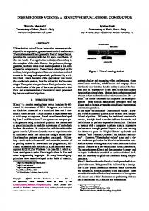
Fig. 5. Relationship between the multi-armed bandit problem and music recommendation.

curve proposed by Ebbinghaus [1913] that measures the user’s memory retention of a song. Novel songs are thus assumed to be those of which a user has little or no memory. Different users can have different recovery rates s. As can be seen from the widespread distribution in Figure 2, some users may repeatedly listen to their favorite songs, while others may be keen to exploring songs they have not listened to previously. Therefore, s is an unknown user parameter to be learned from user interactions. Combined Model. A user’s preference for a recommendation can be represented as a rating; the higher the rating, the more the user likes the recommendation. Unlike traditional recommenders that assume a user’s ratings are static, we assume that a rating is the combined effect of the user’s preference of the song’s content and the dynamically changing novelty. Thus, a song rated as 5 last time could be rated as 2 later because the novelty has decreased. Finally, we define the combined rating model as # " U = Uc Un = θ ′ x 1 − e−t/s . (3) In this model, the more the user likes a particular song, the more likely it will be repeated due to the larger UC value. Also, given that the user’s favorites comprise a small subset of his/her library, the U model behaves in accordance with Zipf ’s Law and ensures that only a small proportion of songs will be frequently repeated. This property of the model will be verified in Section 5.3.2. In Section 5.3.1, we will show that the product form of Eq. (3) leads to significantly better performance than the alternative linear combination U = aUc + bUn. Other Factors. We note that, besides novelty, the repetition of songs can also be affected in other ways. When a user comes to a song of great excitement, he may listen to it again and again. When his interest changes, he may discard songs that he has been frequently repeating. Sometimes, the user finds a song boring initially but repeats it frequently later, while in other cases he may stop repeating a song because he is bored. Understanding and modeling all these factors and precisely predicting when to repeat a song for a particular user would make a very interesting follow-up study. 3.2. Interactive Music Recommendation

Under our rating model, each user is represented by a set of parameters " = {θ, s}. If we knew the values of " of a user, we could simply recommend the songs with the highest rating according to Eq. (3). However, " is hidden and needs to be estimated from historical data, and thus uncertainty always exists. In this case, the greedy strategy used by traditional systems is suboptimal, hence it is necessary to take the uncertainty into account and balance exploration and exploitation. The multi-armed bandit approach introduced in Section 2.2 offers a way to do so for the interactive music recommendation process. As illustrated in Figure 5, we treat ACM Trans. Multimedia Comput. Commun. Appl., Vol. 11, No. 1, Article 7, Publication date: August 2014.

Exploration in Interactive Personalized Music Recommendation

7:9

songs as arms and user ratings as payoffs3 . The music recommendation problem is then transformed into a multi-armed bandit problem and the objective of the music recommender is also changed to maximizing the sum of the ratings given by the target user over the long term. We argue that the cumulative rating is a more realistic objective than the myopic predictive accuracy used by traditional music recommenders, because users generally listen to songs for a long time instead of focusing on one individual song. We adopt the Bayes-UCB algorithm introduced in Section 2.2 for our recommendation task. We denote the rating given by the target user to a recommendation i as a random variable Ri . The expectation of Ri is U given the feature vector (xi , t i ): " # E[Ri ] = Ui = θ ′ xi 1 − e−ti /s . (4)

Then, we develop Bayesian models to estimate the posterior distribution of U given the history recommendation and user ratings. We sketch the framework here and explain it in greater detail in Section 4. We assume that the prior distribution of " is p(") and that, at the (l + 1)-th recommendation, we have accumulated l history recommendations Dl = {(xi , ti , ri )}li=1 as training samples, where ri is the rating given by the user to the i-th recommendation. The posterior distribution of " can then be obtained based on the Bayes’ rule: p("|Dl ) ∝ p(") p(Dl |").

Consequently, the expected rating of song k, denoted as Uk, can be predicted as $ p(Uk|Dl ) = p(Uk|") p("|Dl )d".

(5)

(6)

Henceforth, we will use λlk to denote p(Uk|Dl ) for simplicity. Finally, to balance exploration and exploitation, Bayes-UCB recommends song k∗ that maximizes the quantile function: k∗ = arg maxk=1...|S| Q(α, λlk) where Q satisfies 1 P[Uk ≤ Q(α, λlk)] = α and S is all the songs in the database. We set α = 1 − l+1 following Kaufmann et al. [2012]. The detailed recommendation algorithm is described in Algorithm 1. ALGORITHM 1: Recommendation using Bayes-UCB for l = 1 to n do for all song k = 1, . .". , |S| do # compute qkl = Q 1 − 1/l + 1, λl−1 k end for recommend song k∗ = arg maxk=1...|S| qkl and gather rating rl ; update p("|Dl ) and λlk end for

The cold-start problem is caused by the lack of information required for making good recommendations. There are many ways for mitigating the cold-start problem, most of which rely on additional information about the users or songs, such as popularity/ metadata information about the songs [Hariri et al. 2012] or context/demographic information about the users [Wang et al. 2012]. Although music audio content is required by Uc , it is usually easy to obtain from industry. Our bandit approach addresses the 3 Although

in reality users usually do not give explicit feedback (i.e., ratings) to every recommended song, implicit feedback (e.g., skipping a song, listening to a song fully) can be obtained much more easily. In this article, we focus on explicit feedback to keep the problem simple.

ACM Trans. Multimedia Comput. Commun. Appl., Vol. 11, No. 1, Article 7, Publication date: August 2014.

7:10

X. Wang et al.

Fig. 6. Graphical representation of the Bayesian models. Shaded nodes represent observable random variables, while white nodes represent hidden ones. The rectangle (plate) indicates that the nodes and arcs inside are replicated for N times.

cold-start problem without relying on additional information about users and songs. Instead, it seeks to appropriately explore and exploit information during the whole interactive process. Thus, the bandit approach presents a fundamentally different solution to the cold-start problem, yet can be used in conjunction with the existing methods. There are other Bayesian multi-arm bandit algorithms such as Thompson sampling [Agrawal and Goyal 2012] and optimistic Bayesian sampling [May et al. 2012]. Thompson sampling is based on the probability matching idea, that is, selecting the song according to its probability of being optimal. Optimistic Bayesian sampling uses an exploitative function on top of Thompson sampling. Which of the three is superior? Theoretically, this remains an open question. However, they have been shown to perform comparably well in practice [May et al. 2012]. Existing studies provide little guidance on our selection between them. In this article, we focus on the exploration/ exploitation trade-off principle and simply choose the most recent Bayes-UCB in our implementation. Nevertheless, our system could easily adapt to the other two algorithms as they are also based on the posterior rating distributions. 4. BAYESIAN MODELS AND INFERENCE 4.1. Exact Bayesian Model

To compute Eqs. (5) and (6), we develop the following Bayesian model (see Figure 6(a) for graphical representation). R|x, t, θ , s, σ 2 ∼ N (θ ′ x(1 − e−t/s ), σ 2 ) s ∼ G(d0, e0 )

θ |σ 2 ∼ N (0, c0 σ 2 I)

τ = 1/σ 2 ∼ G( f0 , g0 )

Every part of the model defines a probabilistic dependency between the random variables. N (·, ·) is a (multivariate) Gaussian distribution with the mean and (co)variance parameters, and G(·, ·) is a Gamma distribution with the shape and rate parameters. The rating R is assumed normally distributed following the convention of recommender systems. A gamma prior is put on s because s takes positive values. Following the conventions of Bayesian regression models, a normal prior is put on θ and a Gamma prior on τ . We assume that θ depends on σ 2 because it leads to better convergence in the simulation study. Since there is no closed-form solution to Eq. (5) under this model, Markov Chain Monte Carlo (MCMC) is used as the approximate inference procedure. Directly evaluating Eq. (6) is also infeasible. Thus we use Monte Carlo simulation to obtain λlk: for every sample obtained from the MCMC procedure, we substitute it into Eq. (4) to obtain a sample of Ui , and then use the histogram of the samples of Ui to approximate λlk. This approach is easy to understand and implement. However, it is very slow and users could wait for up to a minute until the Markov chain converges. To make the algorithm more responsive, we develop an approximate Bayesian model and a highly efficient variational inference algorithm in the following sections. ACM Trans. Multimedia Comput. Commun. Appl., Vol. 11, No. 1, Article 7, Publication date: August 2014.

Exploration in Interactive Personalized Music Recommendation

7:11

4.2. Approximate Bayesian Model

4.2.1. Piecewise-Linear Approximation . It is very difficult to develop better inference algorithms for the exact Bayesian model because of the irregular form of the function Un(t). Fortunately, Un can be well approximated by a piecewise-linear function (as shown in Figure 4), thus enabling us to develop an efficient model. For simplicity, we discretize time t into K predetermined intervals: [0, ξ1 ), [ξ1 , ξ2 ), . . . [ξ K−1 , +∞) and only consider the class of piecewise-linear functions whose consecutive line segments intersect at the boundaries of these intervals. This class of functions can be compactly represented as a linear function [Hastie et al. 2009]. We first map t into a vector t = [(t − ξ1 )+ , . . . (t − ξ K−1 ), t, 1], where (t − ξ )+ = max(t − ξ, 0), and then approximate Un(t) as Un(t) ≈ β ′ t, where β = [β1 , . . . β K+1 ]′ is a vector of parameters to be learned from training data. Now, we can represent U as the product of two linear functions: U = Uc Un ≈ θ ′ xβ ′ t. Based on this approximation, we approximate the distributions of R and the parameters of the exact Bayesian model as

R|x, t, θ , β, σ 2 ∼ N (θ ′ xβ ′ t, σ 2 ),

β|σ 2 ∼ N (µβ0 , σ 2 E0 ),

θ |σ 2 ∼ N (µθ0 , σ 2 D0 )

τ = 1/σ 2 ∼ G(a0 , b0 ),

(7)

where θ , β, τ are parameters. D0 , E0 , µθ0 , µβ0 , a0 , b0 are the hyperparameters of the priors to be specified beforehand; D0 and E0 are positive definite matrices. The graphical representation of the model is shown in Figure 6(b). We use conjugate priors for θ , β, τ , which makes the variational inference algorithm described later very efficient. 4.2.2. Variational Inference. Recall that our objective is to compute the posterior distriN bution of parameters " (now it is {θ, β, τ }) given the history data D = {(xi , ti , ri )}i=1 , namely p(θ, β, τ |D). Using piecewise-linear approximation, we now develop an efficient variational inference algorithm. Following the convention of the mean-field approximation [Friedman and Koller 2009], we assume that the joint posterior distribution can be approximated by a restricted distribution q(θ , β, τ ), consisting of three independent factors [Friedman and Koller 2009]:

p("|D) = p(θ, β, τ |D) ≈ q(θ , β, τ ) = q(θ )q(β)q(τ ).

Because of the choice of the conjugate priors, it is easy to show that the restricted distributions q(θ ), q(β), and q(τ ) take the same parametric forms as the prior distributions. Specifically, % & 1 ′ ′ q(θ ) ∝ exp − θ $θ N θ + ηθ N θ , 2

q(τ ) ∝ τ aN −1 exp (−bN τ ) .

% & 1 ′ ′ q(β) ∝ exp − β $β N β + ηβ N β , 2

To find the values that minimize the KL-divergence between q(θ , β, τ ) and the true posterior p(θ , β, τ |D) for the parameters $θ N , ηθ N , $β N , ηβ N , aN , and bN , we use the coordinate descent method. Specifically, we first initialize the parameters of q(θ ), q(β), and q(τ ) and then iteratively update q(θ ), q(β), and q(τ ) until the variational lower bound L (elaborated in Appendix C) converges. Further explanation about the principle can be found in Friedman and Koller [2009]. The detailed steps are described in Algorithm 2, where p and K are the dimensionalities of x and t, respectively; the moments of θ, β, τ are derived in Appendix B. ACM Trans. Multimedia Comput. Commun. Appl., Vol. 11, No. 1, Article 7, Publication date: August 2014.

7:12

X. Wang et al.

ALGORITHM 2: Variational inference input: D, D0 , E0 , µθ 0 , µβ0 , a0 , b0 initialize $θ N , ηθ N , $β N , ηβ N , aN , bN repeat ' ' * * ( ′) !N !N ′ ′ ′ update q(θ): $θ N ← E[τ ] D−1 ηθ N ← E[τ ] D−1 i=1 xi ti E ββ ti xi , i=1 ri xi ti E[β] 0 + 0 µθ0 + * ' ' * !N !N ′ ′ ′ ′ ηβ N ← E[τ ] E−1 update q(β): $β N ← E[τ ] E−1 i=1 ti xi E[θ θ ]xi ti , i=1 ri ti xi E[θ ] 0 + 0 µβ0 +

+ a0 , update q(τ ): aN ← p+K+N 2 , 1+ + * , , " # " # #, ' 1 + + −1 " tr E−1 bN ← tr D0 E[θθ ′ ] + µ′θ0 − 2E[θ ]′ D−1 E[ββ ′ ] + µ′β0 − 2E[β]′ E−1 µθ 0 + µβ0 0 0 0 2 2 N N * 1 -' 2 + ri xi′ E[θ]ti′ E[β] + b0 ri + xi′ E[θθ T ]xi ti′ E[ββ T ]ti − 2 i=1

i=1

until L converges return $θ N , ηθ N , $β N , ηβ N , aN , bN

4.2.3. Predict the Posterior Distribution p (U|D). Because q(θ ) and q(β) are normal distributions, θ ′ x and β ′ t are also normally distributed " # " # ′ −1 ′ −1 p(θ ′ x|x, t, D) ≈ N x′ $−1 p(β ′ t|x, t, D) ≈ N t′ $−1 θ N η θ N , x $θ N x , β N η β N , t $β N t ,

and the posterior distribution of U in Eq. (6) can be computed as & % $ U p(θ ′ x = a|x, t, D) p β ′ t = |x, t, D da. p(U |x, t, D) = p(θ ′ xβ ′ t|x, t, D) = a

Since there is no closed-form solution to the preceding integration, we use Monte Carlo simulation. Namely, we first obtain one set of samples for each of θ ′ x and β ′ t and then use the elementwise products of the two groups of samples to approximate the distribution of U . Because θ ′ x and β ′ t are normally distributed univariate random variables, the sampling can be very efficiently done. Moreover, the prediction for different songs is trivially parallelizable and thus scalable. 4.2.4. Integration of Other Factors. Although the approximate model considers music audio content and novelty only, it is easy to incorporate other factors as long as they can be approximated by linear functions. For instance, diversity is another important factor for a playlist. We could measure the diversity that a song contributes to a playlist as d and assume the user preference for d follows a function that can be approximated by a piecewise-linear function. Following the method in Section 4.2.1, we can map d into a vector d and modify the approximate Bayesian model in Section 4.2.1 by adding an additional term γ ′ d to Eq. (7) and putting a prior on γ as shown in the following: # " R|x, t, d, σ 2 , θ , β, γ ∼ N (θ ′ xβ ′ tγ ′ d, σ 2 ), γ |σ 2 ∼ N µγ 0 , σ 2 F0 .

Given the symmetry between x, t, and d, we can modify Algorithm 2 without further derivation. Similarly, we could incorporate more factors such as coherence of mood and genre into the model. Moreover, the model can also be applied to other regression tasks as long as the regression function can be factorized into the product of a few linear functions.

5. EXPERIMENTS

We compare the results from our evaluations of six recommendation algorithms in this section. Extensive experimental evaluations of both efficiency and effectiveness of the ACM Trans. Multimedia Comput. Commun. Appl., Vol. 11, No. 1, Article 7, Publication date: August 2014.

Exploration in Interactive Personalized Music Recommendation

7:13

algorithms and models have been conducted and the results show significant promise from both aspects. 5.1. Experiment Setup

5.1.1. Compared Recommendation Algorithms. To study the effectiveness of the exploration/exploitation trade-off, we introduced two baselines, Random and Greedy. The Random approach represents pure exploration and recommends songs uniformly at random. The Greedy approach represents pure exploitation and always recommends the song with the highest predicted rating. Therefore, the Greedy approach simulates the strategy used by traditional recommenders, where the parameters {θ, s} were estimated by minimizing the mean square error using the L-BFGS-B algorithm [Byrd et al. 1995]. To study the effectiveness of the rating model, we introduced a baseline using LinUCB, a bandit algorithm that assumes the expected rating is a linear function of the feature vector [Li et al. 2012]. In LinUCB, ridge regression served as the regression method and the upper confidence bound is used to balance exploration and exploitation. Two combinations of the factors Uc and Un were evaluated: Uc and Uc Un. We denote them as C and CN for short, where C and N indicate content and novelty, respectively. For example, Bayes-UCB-CN contains both content and novelty. Furthermore, BayesUCB-CN corresponds to the exact Bayesian model with the MCMC inference algorithm (Section 4.1), whereas Bayes-UCB-CN-V the approximate model with the variational inference algorithm (Section 4.2). We evaluated six recommendation algorithms that were combinations of the four approaches and three factors: Random, LinUCB-C, LinUCB-CN, Bayes-UCB-CN, BayesUCB-CN-V, and Greedy-CN. Because LinUCB-CN cannot handle nonlinearity and thus cannot directly model Uc Un, we combined the feature vector x in Uc and the time variable t in Un as one vector and treated the expected rating as a linear function of the combined vector. Greedy-C was not included because it was not related to our objective. As discussed in Section 3.2, the bandit approach can also be combined with existing methods to solve the cold-start problem. We plan to study the effectiveness of such combinations in future works. 5.1.2. Songs and Features. Ten thousand songs from different genres were used in the experiments. Videos of the songs were crawled from YouTube and converted by ffmpeg4 into mono channel WAV files with a 16 kHz sampling rate. For every song, a 30s audio clip was used [Wang et al. 2012]. Feature vectors were then extracted using a program developed based on the MARSYAS library5 , in which a window size of 512 was used without overlapping. The features used (and their dimensionalities) are Zero Crossing Rate (1), Spectral Centroid (1), Spectral Rolloff (1), Spectral Flux (1), MFCC (13), Chroma (14), Spectral Crest Factor (24), and Spectral Flatness Measure (24). Detailed descriptions of these features are given in Table II in the Appendix. The features have been commonly used in the music retrieval/recommendation domain [Cano et al. 2005; Yoshii et al. 2006; Wang et al. 2012]. To represent a 30s clip in one feature vector, we used the mean and standard deviation of all feature vectors from the clip. Next, we added the one-dimensional feature tempo to the summarized feature vectors. The resulting feature dimensionality is 79 × 2 + 1 = 159. Directly using the 159-dimensional features requires a large amount of data to train the models and makes user studies very expensive and time consuming. To reduce the dimensionality, 4 http://ffmpeg.org.

5 http://marsyas.sourceforge.net.

ACM Trans. Multimedia Comput. Commun. Appl., Vol. 11, No. 1, Article 7, Publication date: August 2014.

7:14

X. Wang et al.

we conducted Principal Component Analysis (PCA) with 90% of variance reserved. The final feature dimensionality is thus reduced to 91. The performance of these features in music recommendation was checked based on a dataset that we built. We did not use existing music recommendation datasets because they lack explicit ratings and dealing with implicit feedback is not our focus. Fifty-two undergraduate students with various cultural backgrounds contributed to the dataset, with each student annotating 400 songs with a 5-point Likert scale from “very bad” (1) to “very good” (5). We computed the tenfold cross-validation RMSE of Uc for each user and averaged the accuracy over all users. The resulting RMSE is 1.10, significantly lower than the RMSE (1.61) of the random baseline with the same distribution as the data. Therefore, these audio features indeed provide useful information for recommendation. The accuracy can be further improved by feature engineering [Oord et al. 2013], which we reserve for future work. 5.1.3. Evaluation Protocol. In Li et al. [2011], an offline approach is proposed for evaluating contextual bandit approaches with the assumption that the context (including the audio features and the elapsed time of songs) at different iterations is identically independently distributed. Unfortunately, this is not true in our case because when a song is not recommended, its elapsed time t keeps increasing and is thus strongly correlated. Therefore, an online user study is the most reliable means of evaluation. To reduce the cost of the user study, we first conducted a comprehensive simulation study to verify the approaches. We then proceeded to user study for further verification only if they passed the simulations. The whole process underwent a few iterations, during which the models and algorithms were continually refined. The results hereby presented are from the final iteration. Intermediate results are either referred to as preliminary study whenever necessary or omitted due to page limitation. 5.2. Simulations

5.2.1. Effectiveness Study. U = Uc Un was used as the true model because the preliminary user studies showed that this resulted in better performance, which will be verified in Section 5.3 again. Because our model considers the impact of time, to make the simulations close to real situations, songs were rated about 50s after being recommended. We treated every 20 recommendations as a recommendation session, and the sessions were separated by four-minute gaps. Priors for the Bayesian models were set as uninformative ones or chosen based on preliminary simulation and user studies. For the exact Bayesian model, they are: c0 = 10, d0 = 3, e0 = 10−2 , f0 = 10−3 , g0 = 10−3 , where f0 , g0 are uninformative and c0 , d0 , e0 are based on preliminary studies. For the approximate Bayesian model, they are: D0 = E0 = 10−2 I, µθ 0 = µβ0 = 0, a0 = 2, b0 = 2 × 10−8 , where µθ 0 , µβ0 , a0 , b0 are uninformative and D0 , E0 are based on preliminary studies; I is the identity matrix. Un was discretized into the following intervals (in minutes) according to the exponentially decaying characteristics of human memory [Ebbinghaus 1913]: [0, 2−3 ), [2−3 , 2−2 ), . . . , [210 , 211 ), [211 , +∞). We defined the smallest interval as [0, 2−3 ) because people usually do not listen to a song for less than 2−3 minutes (7.5s). The largest interval was defined as [211 , +∞) because our preliminary user study showed that evaluating one algorithm takes no more than 1.4 day, namely approximately 211 minutes. Further discretization of [211 , +∞) should be easy. For songs that had not been listened to by the target user, the elapsed time t was set as one month to ensure that Un is close to 1. We compared the performance of the six recommendation algorithms in terms of regret, a widely used metric in the RL literature. First we define that, for the l-th ACM Trans. Multimedia Comput. Commun. Appl., Vol. 11, No. 1, Article 7, Publication date: August 2014.

Exploration in Interactive Personalized Music Recommendation

Fig. 7. Regret comparison in simulation.

7:15

Fig. 8. Time efficiency comparison.

recommendation, the difference between the maximum expected rating E[ Rˆ l ] = l ˆl maxk=1...|S| Uk and the expected rating of the recommended song is (l = E[ !R ] − E[R ]. Then, the cumulative regret for the n-th recommendation is: Rn = ( l=1...n l = ! l l ˆ l=1...n E[ R ] − E[R ], where a smaller Rn indicates better performance. Different values of parameters {θ , s} were tested. Elements of θ were sampled from the standard normal distribution and s was sampled from the uniform distribution with the range (100, 1000), where the range was determined based on the preliminary user study. We conducted ten runs of the simulation study. Figure 7 shows the means and standard errors of the regret of different algorithms at different numbers of recommendations n. From the figure, we see that the algorithm Random (pure exploration) performs the worst. The two LinUCB-based algorithms are worse than Greedy-CN because LinUCB-C does not capture the novelty and LinUCB-CN does not capture the nonlinearity within Uc and Un although both LinUCB-C and LinUCB-CN balance exploration and exploitation. Bayes-UCB-based algorithms performed better than Greedy-CN because Bayes-UCB balances exploration and exploitation. In addition, the difference between Bayes-UCB and Greedy increases very fast when n is small. This is because small n means a small number of training samples and results in high uncertainty, that is, the cold-start stage. Greedy algorithms, which are used by most existing recommendation systems, do not handle the uncertainty well, while Bayes-UCB can reduce the uncertainty quickly and thus improves the recommendation performance. The good performance of Bayes-UCBCN-V also indicates that the piecewise-linear approximation and variational inference are accurate. 5.2.2. Efficiency Study. A theoretical efficiency study of MCMC and variational inference algorithms is difficult to analyze due to their iterative nature and deserves future work. Instead, we conducted an empirical efficiency study of the training algorithms for Bayes-UCB-CN (MCMC), Bayes-UCB-CN-V (variational inference), and GreedyCN (L-BFGS-B). In addition, the variational inference algorithm for the three-factor model described in Section 4.2.4 was also studied. LinUCB and Random were not included because the algorithms are much simpler and thus faster (but also perform much worse). Experiments were conducted on a computer with an Intel Xeon CPU (L5520 @ 2.27 GHz) and 32GB main memory. No multithreading or GP-GPU were used in the comparisons. The programming language R was used to implement all the six algorithms. From the results in Figure 8, we can see that the time consumed by both MCMC and variational inference grows linearly with the training set size. However, variational ACM Trans. Multimedia Comput. Commun. Appl., Vol. 11, No. 1, Article 7, Publication date: August 2014.

7:16

X. Wang et al.

Fig. 9. Accuracy versus training time.

Fig. 10. Sample efficiency comparison.

inference is more than 100 times faster than the MCMC, and significantly faster than the L-BFGS-B algorithm. Comparing the variational inference algorithm with two or three factors, we find that adding another factor to the approximate Bayesian model only slightly slows down the variational inference algorithm. Moreover, when the sample size is less than 1000, the variational inference algorithm can finish in 2s, which makes online updating practical and well meets the user requirement. Implementing the algorithms in more efficient languages like C/C++ can result in even better efficiency. The training time of all the algorithms is also affected by the accuracy that we want to achieve. To study this, we generated a training set (350 samples) and a test set (150 samples). For each algorithm, we ran it on the training set multiple times. Every time we used a different number of training iterations and collected both the training time and prediction accuracy on the test set. The whole process was repeated ten times. For each algorithm and each number of iterations, the ten training times and prediction accuracies were averaged. From the results shown in Figure 9, we can see that variational inference (VI) converges very fast; L-BFGS-B takes much longer time than VI to converge, while MCMC is more than 100 times slower than VI. Time consumed in the prediction phase of the Bayesian methods is larger than that of Greedy- and LinUCB-based methods because of the sampling process. However, for the two-factors model Bayes-UCB-CN-V, prediction can be accelerated significantly by the PRODCLIN algorithm without sacrificing the accuracy [MacKinnon et al. 2007]. In addition, since prediction for different songs is trivially parallelizable, scaling variational inference to large music databases should be easy. We also conducted a sample efficiency study of the exact Bayesian model, the approximate Bayesian model, and the minimum mean-squared-error-based frequentist model used for Greedy-CN. We first generated a test set (300 samples) and then tested all the models with different sizes of training samples. The whole process was repeated ten times and the average accuracies are shown in Figure 10. We can see that the exact Bayesian model and the frequentist model have almost identical sample efficiency, confirming that the only difference between Bayes-UCB and Greedy-CN is whether uncertainty is considered. The approximate Bayesian model performs slightly worse than the others because of the piecewise-linear approximation and the variational inference algorithm. 5.3. User Study

Undergraduate students aged 17–25 years were chosen as our study target. It would be interesting to study the impact of occupations and ages on our method in the future. ACM Trans. Multimedia Comput. Commun. Appl., Vol. 11, No. 1, Article 7, Publication date: August 2014.

Exploration in Interactive Personalized Music Recommendation

Fig. 11. User evaluation interface.

7:17

Fig. 12. Performance comparison in user study.

Most applicants were females, and we selected 15 from them with approximately equal number of males (6) and females (9). Their cultural backgrounds were diversified to include Chinese, Malay, Indian, and Indonesian. They all listen to music regularly (at least three hours per week). To reduce the number of subjects needed, the withinsubject experiment design was used, that is, every subject evaluated all recommendation algorithms. Every subject was rewarded with a small token payment for her time and effort. For each of the six algorithms, a subject evaluated 200 recommendations, a number more than sufficient to cover the cold-start stage. Every recommended song was listened to for at least 30s (except when the subject was very familiar with the song a priori) and rated based on a 5-point Likert scale as before. Subjects were required to rest for at least four minutes after listening to 20 songs to ensure the quality of the ratings and simulate recommendation sessions. To minimize the carryover effect of the within-subject design, subjects were not allowed to evaluate more than two algorithms within one day. Moreover, there must be a gap of more than six hours between two algorithms. The user study lasted one week. Every subject spent more than 14 hours in total. The dataset will be released after the publication of this article. During the evaluation, the recommendation models were updated immediately whenever a new rating was obtained. The main interface used for evaluation is in Figure 11. 5.3.1. The Overall Recommendation Performance. Because the true model is not known in the user study, the regret used in simulations cannot be used here. We thus choose the average rating as the evaluation metric, which is also popular in evaluations of RL algorithms. Figure 12 shows the average ratings and standard errors of every algorithm from the beginning to the n-th recommendation. T-tests at different iterations show Bayes-UCB-CN outperforms Greedy-CN since the 45th iteration with p-values < 0.039. Bayes-UCB-CN-V outperforms Greedy-CN from the 42nd to the 141st iteration with p-values < 0.05, and afterwards with pvalues < 0.1. Bayes-UCB-CN and Greedy-CN share the same rating model and the only difference between them is that Bayes-UCB-CN balances exploration/exploitation while Greedy-CN only exploits. Therefore, the improvement of Bayes-UCB-CN over Greedy-CN is solely contributed by the exploration/exploitation trade-off. More interestingly, when n ≤ 100 (cold-start stage) the differences between BayesUCB-CN and Greedy-CN are even more significant. This is because, during the coldstart stage, the uncertainty is very high; Bayes-UCB explores and thus reduces the uncertainty quickly while Greedy-CN always exploits and thus cannot reduce the uncertainty as efficiently as Bayes-UCB-CN. To verify this point, we first define a 1 !|S| metric for uncertainty as |S| k=1 SD[ p(Uk|Dn)], which is the mean of the standard ACM Trans. Multimedia Comput. Commun. Appl., Vol. 11, No. 1, Article 7, Publication date: August 2014.

7:18

X. Wang et al.

Fig. 13. Uncertainty.

deviations of all songs’ posterior distributions p(Uk|Dn) estimated using the exact Bayesian model. Larger standard deviation means larger uncertainty as illustrated in Figure 1. Given the iteration n, we calculate an uncertainty measure based on each user’s recommendation history. The means and standard errors of the uncertainties among all users at different iterations are shown in Figure 13. When the number of training data points increases, the uncertainty decreases. Also as expected, the uncertainty of Bayes-UCB-CN decreases faster than Greedy-CN when n is small, and later the two remain comparable because both have obtained enough training samples to fully train the models. This verifies that our bandit approach handles uncertainty better during the initial stage, thus mitigating the cold-start problem. Results in Figure 12 also show that all algorithms involving CN outperform LinUCBC, indicating that the novelty factor of the rating model improves recommendation performance. In addition, Bayes-UCB-CN outperforms LinUCB-CN significantly, suggesting that multiplying Uc and Un together works better than linearly combining them. 5.3.2. Playlist Generation. As discussed in Section 3.1, repeating songs following the Zipf ’s law is important for playlist generation. Therefore, we evaluated the playlists generated during the recommendation process by examining the distribution of song repetition frequencies for every user. We generated the plots of the distributions in the same way we generated Figure 3 for the six algorithms. Ideal algorithms should reproduce repetition distributions of Figure 3. The results of the six algorithms are shown in Figure 14. As we can see, all algorithms with Uc and Un multiplied together (i.e., Bayes-UCB-CN, Greedy-CN, BayesUCB-CNV) reproduce the Zipf ’s law pattern well, while the algorithms without Uc (Random, LinUCB-C) or with Uc and Un added together (LinUCB-CN) do not. This confirms that our model U = Uc Un can effectively reproduce the Zipf ’s law distribution. Thus, we successfully modeled an important part for combining music recommendation and playlist generation. 5.3.3. Piecewise-Linear Approximation. In addition to the studies detailed previously, the piecewise-linear approximation of the novelty model is tested again by randomly selecting four users and showing in Figure 15 their novelty models learned by BayesUCB-CN-V. Specifically, the posterior distributions of β ′ t for t ∈ (0, 211 ) are presented. The lines represent the mean values of β ′ t and the regions around the lines the confidence bands of one standard deviation. The scale of β ′ t is not important because β ′ t is multiplied together with the content factor, and any constant scaling of one factor can ACM Trans. Multimedia Comput. Commun. Appl., Vol. 11, No. 1, Article 7, Publication date: August 2014.

Exploration in Interactive Personalized Music Recommendation

7:19

Fig. 14. Distributions of song repetition frequency.

Fig. 15. Four users’ diversity factors learned from the approximate Bayesian model.

be compensated by the scaling of the other one. Comparing Figure 15 and Figure 4, we can see that the learned piecewise-linear novelty factors well match our analytic form Un. This again confirms the accuracy of the piecewise-linear approximation. 6. DISCUSSION

Exploring user preferences is a central issue for recommendation systems, regardless of the specific media types. Under uncertainty, the greedy approach usually produces suboptimal results and balancing exploration/exploitation is important. One successful example of the exploration/exploitation trade-off is the news recommender [Li et al. 2012]. Our work in this article has shown its effectiveness in music recommendation. Given that uncertainty exists universally in all kinds of recommenders, it will be interesting to examine its effectiveness in recommenders for other media types, such as video and image. Our models and algorithms could be generalized to other recommenders. First, the mathematical form of the approximate Bayesian model is general enough to cover a family of rating functions that can be factorized as the product of a few linear functions (Section 4.2.4). Moreover, we can often approximate nonlinear functions with linear ones. For instance, we can use a feature mapping function φ(x) and make Uc = θ ′ φ(x) to capture the nonlinearity in our content model. Therefore, it will be interesting to explore our approximate Bayesian model and the variational inference algorithm in other recommendation systems. Second, the proposed novelty model may not be suitable for movie recommendation due to different consumption patterns in music and movies. In other words, users may listen to their favorite songs many times, but repetitions are relatively rare for movies. However, the novelty model may suit recommenders that repeat items (e.g., food or makeup recommenders [Liu et al. 2013]). ACM Trans. Multimedia Comput. Commun. Appl., Vol. 11, No. 1, Article 7, Publication date: August 2014.

7:20

X. Wang et al.

If their repetition patterns also follow the Zipf ’s law, both the exact and approximate Bayesian models can be used; otherwise, the approximate Bayesian model can be used. As for extensions of this work, the first interesting direction is to model the correlations between different users to further reduce the amount of exploration. This could be achieved by extending the Bayesian models to hierarchical Bayesian models. Another interesting direction is to consider more factors such as diversity, mood, and genres to generate even better playlists. For people who prefer CF, a future direction could be to use the exploration/ exploitation trade-off idea to boost CF’s performance. A simple approach is to use the latent features learned by existing matrix factorization methods to replace the audio features in our methods and keep other parts of our methods unchanged. 7. CONCLUSION

In this article, we described a multi-armed bandit approach to interactive music recommendation that balances exploration and exploitation, mitigates the cold-start problem, and improves recommendation performance. We described a rating model including music audio content and novelty to integrate music recommendation and playlist generation. To jointly learn the parameters of the rating model, a Bayesian regression model together with an MCMC inference procedure were developed. To make the Bayesian inference efficient enough for online updating and generalize the model for more factors such as diversity, a piecewise-linear approximate Bayesian regression model and a variational inference algorithm were built. The results from simulation demonstrate that our models and algorithms are accurate and highly efficient. User study results show that: (1) the bandit approach mitigates the cold-start problem and improves recommendation performance, and (2) the novelty model together with the content model capture the Zipf ’s law of repetitions in recommendations. REFERENCES S. Agrawal and N. Goyal. 2012. Analysis of thompson sampling for the multi-armed bandit problem. In Proceedings of the 25th Annual Conference on Learning Theory (COLT’12). N. Aizenberg, Y. Koren, and O. Somekh. 2012. Build your own music recommender by modeling internet radio streams. In Proceedings of the 21st International Conference on World Wide Web (WWW’12). ACM Press, New York, 1–10. P. Auer. 2003. Using confidence bounds for exploitation-exploration trade-offs. J. Mach. Learn. Res. 3, 397– 422. M. Braunhofer, M. Kaminskas, and F. Ricci. 2013. Location-aware music recommendation. Int. J. Multimedia Inf. Retr. 2, 1, 31–44. R. H. Byrd, P. Lu, J. Nocedal, and C. Zhu. 1995. A limited memory algorithm for bound constrained optimization. SIAM J. Sci. Comput. 16, 5, 1190–1208. P. Cano, M. Koppenberger, and N. Wack. 2005. Content-based music audio recommendation. In Proceedings of the 13th Annual ACM International Conference on Multimedia (MM’05). ACM Press, New York, 211–212. P. Castells, S. Vargas, and J. Wang. 2011. Novelty and diversity metrics for recommender systems: Choice, discovery and relevance. In Proceedings of the International Workshop on Diversity in Document Retrieval (DDR’11) at the 33rd European Conference on Information Retrieval (ECIR’11). 29–36. H. C. Chen and A. L. P. Chen. 2001. A music recommendation system based on music data grouping and user interests. In Proceedings of the 10th International Conference on Information and Knowledge Management (CIKM’01). ACM Press, New York, 231–238. S. Chen, J. L. Moore, D. Turnbull, and T. Joachims. 2012. Playlist prediction via metric embedding. In Proceedings of the 18th ACM SIGKDD International Conference on Knowledge Discovery and Data Mining (KDD’12). 714–722. X. Chen, P. N. Bennett, K. Collins-Thompson, and E. Horvitz. 2013. Pairwise ranking aggregation in a crowdsourced setting. In Proceedings of the 6th ACM International Conference on Web Search and Data Mining (WSDM’13). ACM Press, New York, 193–202. ACM Trans. Multimedia Comput. Commun. Appl., Vol. 11, No. 1, Article 7, Publication date: August 2014.

Exploration in Interactive Personalized Music Recommendation

7:21

Z. Cheng and J. Shen. 2014. Just-for-me: An adaptive personalization system for location-aware social music recommendation. In Proceedings of International Conference on Multimedia Retrieval (ICMR’14). 185. C. Y. Chi, R. T. H. Tsai, J. Y. Lai, and J. Y. Jen Hsu. 2010. A reinforcement learning approach to emotionbased automatic playlist generation. In Proceedings of the International Conference on Technologies and Applications of Artificial Intelligence. IEEE Computer Society, 60–65. H. Ebbinghaus. 1913. Memory: A Contribution to Experimental Psychology. Educational reprints. Teachers College, Columbia University. D. Eck, P. Lamere, T. Bertin-Mahieux, and S. Green. 2007. Automatic generation of social tags for music recommendation. In Proceedings of the Neural Information Processing Systems Conference (NIPS’07). Vol. 20. N. Friedman and D. Koller. 2009. Probabilistic Graphical Models: Principles and Techniques 1st Ed. The MIT Press. N. Golovin and E. Rahm. 2004. Reinforcement learning architecture for web recommendations. In Proceedings of the International Conference on Information Technology: Coding and Computing. Vol. 1, IEEE, 398–402. A. Gunawardana and G. Shani. 2009. A survey of accuracy evaluation metrics of recommendation tasks. J. Mach. Learn. Res 10, 2935–2962. N. Hariri, B. Mobasher, and R. Burke. 2012. Context-aware music recommendation based on latenttopic sequential patterns. In Proceedings of the 6th ACM Conference on Recommender Systems (RecSys’12). ACM Press, New York, 131–138. T. Hastie, R. Tibshirani, and J. Friedman. 2009. The Elements of Statistical Learning. Springer. Y. Hu and M. Ogihara. 2011. Nextone player: A music recommendation system based on user behavior. In Proceedings of the 12th International Society for Music Information Retrieval Conference (ISMIR’11). T. Joachims, D. Freitag, and T. Mitchell. 1997. WebWatcher: A tour guide for the world wide web. In Proceedings of the 15th International Joint Conference on Artificial Intelligence (IJCAI’97). 770–777. M. Kaminskas, F. Ricci, and M. Schedl. 2013. Location-aware music recommendation using auto-tagging and hybrid matching. In Proceedings of the 7th ACM Conference on Recommender Systems (RecSys’13). ACM Press, New York, 17–24. R. Karimi, C. Freudenthaler, A. Nanopoulos, and L. Schmidt-Thieme. 2011. Towards optimal active learning for matrix factorization in recommender systems. In Proceedings of the 23rd IEEE International Conference on Tools with Artificial Intelligence (ICTAI’11). 1069–1076. E. Kaufmann, O. Capp´e, and A. Garivier. 2012. On bayesian upper confidence bounds for bandit problems. J. Mach. Learn. Res. Proc. Track 22, 592–600. P. Knees and M. Schedl. 2013. A survey of music similarity and recommendation from music context data. ACM Trans. Multimedia Comput. Comm. Appl. 10, 1. Y. Koren, R. Bell, and C. Volinsky. 2009. Matrix factorization techniques for recommender systems. Comput. 42, 8, 30–37. N. Lathia, S. Hailes, L. Capra, and X. Amatriain. 2010. Temporal diversity in recommender systems. In Proceedings of the 33rd International ACM SIGIR Conference (SIGIR’10). ACM Press, New York, 210– 217. L. Li, W. Chu, J. Langford, and R. E. Schapire. 2012. A contextual-bandit approach to personalized news article recommendation. In Proceedings of the 19th International Conference on World Wide Web (WWW’10). ACM Press, New York, 661–670. L. Li, W. Chu, J. Langford, and X. Wang. 2011. Unbiased offline evaluation of contextual-bandit-based news article recommendation algorithms. In Proceedings of the 4th ACM International Conference on Web Search and Data Mining (WSDM’11). ACM Press, New York, 297–306. E. Liebman and P. Stone. 2014. Dj-mc: A reinforcement-learning agent for music playlist recommendation. http://arxiv.org/pdf/1401.1880.pdf H. Liu, J. Hu, and M. Rauterberg. 2009. Music playlist recommendation based on user heartbeat and music preference. In Proceedings of the International Conference on Computer Technology and Development. Vol. 1, 545–549. L. Liu, H. Xu, J. Xing, S. Liu, X. Zhou, and S. Yan. 2013. Wow! You are so beautiful today! In Proceedings of the 21st ACM International Conference on Multimedia (MM’13). 3–12. B. Logan. 2002. Content-based playlist generation: Exploratory experiments. In Proceedings of the 3rd International Conference on Music Information Retrieval (ISMIR’02). 295–296. D. P. Mackinnon, M. S. Fritz, J. Williams, and C. M. Lockwood. 2007. Distribution of the product confidence limits for the indirect effect: Program prodclin. Behav. Res. Methods 39, 3, 384–389.

ACM Trans. Multimedia Comput. Commun. Appl., Vol. 11, No. 1, Article 7, Publication date: August 2014.

7:22

X. Wang et al.

B. C. May, N. Korda, A. Lee, and D. S. Leslie. 2012. Optimistic bayesian sampling in contextual-bandit problems. J. Mach. Learn. Res. 13, 1, 2069–2106. M. E. J. Newman. 2005. Power laws, pareto distributions and zipf ’s law. Contemp. Phys. 46, 5, 323–351. A. V. D. Oord, S. Dieleman, and B. Schrauwen. 2013. Deep content-based music recommendation. In Proceedings of the Conference on Advances in Neural Information Processing Systems (NIPS’13). 2643–2651. R. Salakhutdinov and A. Mnih. 2008. Bayesian probabilistic matrix factorization using markov chain monte carlo. In Proceedings of the 25th International Conference on Machine Learning (ICML’08). ACM Press, New York, 880–887. M. Schedl and D. Schnitzer. 2014. Location-aware music artist recommendation. In Proceedings of the 20th International Conference on MultiMedia Modeling (MMM’14). G. Shani, D. Heckerman, and R. I. Brafman. 2005. An mdp-based recommender system. J. Mach. Learn. Res 6, 1265–1295. J. Shen, X. S. Hua, and E. Sargin. 2013. Towards next generation multimedia recommendation systems. In Proceedings of the 21st ACM International Conference on Multimedia (MM’13). ACM Press, New York, 1109–1110. J. Silva and L. Carin. 2012. Active learning for online bayesian matrix factorization. In Proceedings of the 18th ACM SIGKDD International Conference on Knowledge Discovery and Data Mining (KDD’12). ACM Press, New York, 325–333. Y. Song, S. Dixon, and M. Pearce. 2012. A survey of music recommendation systems and future perspectives. In Proceedings of the 9th International Symposium on Computer Music Modelling and Retrieval (CMMR’12). A. Srivihok and P. Sukonmanee. 2005. E-commerce intelligent agent: Personalization travel support agent using q learning. In Proceedings of the 7th International Conference on Electronic Commerce (ICEC’05). ACM Press, New York, 287–292. R. S. Sutton and A. G. Barto. 1998. Reinforcement Learning: An Introduction. Bradford. ´ 2010. Algorithms for Reinforcement Learning. Synthesis Lectures on Artificial Intelligence and C. Szepesvari. Machine Learning Series. Vol. 4, Morgan and Claypool, San Rafael, CA. N. Taghipour and A. Kardan. 2008. A hybrid web recommender system based on q-learning. In Proceedings of the ACM Symposium on Applied Computing (SAC’08). 1164–1168. X. Wang, D. Rosenblum, and Y. Wang. 2012. Context-aware mobile music recommendation for daily activities. In Proceedings of the 20th ACM International Conference on Multimedia (MM’12). ACM Press, New York, 99–108. K. Yoshii, M. Goto, K. Komatani, T. Ogata, and H. G. Okuno. 2006. Hybrid collaborative and content-based music recommendation using probabilistic model with latent user preferences. In Proceedings of the 7th International Conference on Music Information Retrieval (ISMIR’06). 296–301. B.-T. Zhang and Y.-W. Seo. 2001. Personalized web-document filtering using reinforcement learning. Appl. Artif. Intell. 15, 665–685. Y. C. Zhang, Diarmuid, D. Quercia, and T. Jambor. 2012. Auralist: Introducing serendipity into music recommendation. In Proceedings of the 5th ACM International Conference on Web Search and Data Mining (WSDM’12). ACM Press, New York, 13–22. E. Zheleva, J. Guiver, E. M. Rodrigues, and N. M. Frayling. 2010. Statistical models of music-listening sessions in social media. In Proceedings of the 19th International Conference on World Wide Web (WWW’10). ACM Press, New York, 1019–1028. Received November 2013; revised May 2014; accepted May 2014

ACM Trans. Multimedia Comput. Commun. Appl., Vol. 11, No. 1, Article 7, Publication date: August 2014.

Online Appendix to: Exploration in Interactive Personalized Music Recommendation: A Reinforcement Learning Approach XINXI WANG, National University of Singapore YI WANG, Institute of High Performance Computing, A*STAR DAVID HSU and YE WANG, National University of Singapore In this online appendix, we present conditional distributions for the approximate Bayesian model, variational inference, and the variational lower bound. A. CONDITIONAL DISTRIBUTIONS FOR THE APPROXIMATE BAYESIAN MODEL N Given N training samples D = {ri , xi , ti }i=1 , the conditional distribution p(θ|D, τ, β) remains a normal distribution:

p(θ |D, τ, β) ∝ p(τ ) p(θ|τ ) p(β|τ ) ∝ p(θ|τ )

N ! i=1

N ! i=1

p(ri |xi , ti , θ , β, τ ),

p(ri |xi , ti , θ , β, τ ),

# " 1 ′ 2 −1 ∝ exp − (θ − µθ0 ) (σ D0 ) (θ − µθ0 ) 2 $ N & % 1 ′ ′ 2 2 −1 − (ri − xi θ ti β) (σ ) exp , 2 i=1 $ & $ & ( ' N N % % 1 ′ ′ ′ −1 −1 ′ ′ ′ ′ xi ti ββ ti xi θ + τ µθ0 D0 + ri β ti xi θ , ∝ exp − θ τ D0 + τ 2 i=1 i=1 # " 1 ′ ′ ∝ exp − θ #θ N θ + ηθ N θ , 2 where #θ N = τ η′θ N

=τ

$

D−1 0

$

+

N %

xi ti′ ββ ′ ti xi′

i=1

µ′θ0 D−1 0

+

N % i=1

ri β

′

ti xi′

&

&

.

Due to the symmetry between θ and β, we can easily obtain " # 1 ′ ′ p(β|D, τ, θ ) ∝ exp − β #β N β + ηβ N β , 2 c 2014 ACM 1551-6857/2014/08-ART7 $15.00 ⃝ DOI: http://dx.doi.org/10.1145/2623372 ACM Trans. Multimedia Comput. Commun. Appl., Vol. 11, No. 1, Article 7, Publication date: August 2014.

App–2

X. Wang et al.

where !

!β N = τ E0 η′β N

=τ

−1

!

+

N "

ti xi′ θ θ ′ xi ti′

i=1

µ′β0 E0 −1

+

N "

ri θ

′

#

xi ti′

i=1

#

.

The conditional distribution p(τ |D, θ , β) also remains a Gamma distribution p(τ |D, θ, β) ∝ τ aN −1 exp (−bN τ ) , p(τ |D, θ, β) ∝ p(τ ) p(θ|τ ) p(β|τ )

N $ i=1

p(ri |xi , ti , θ , β, τ ),

1 τ a0 −1 exp(−b0 τ ), "(a0 ) & % 1 1 ′ 2 −1 exp − (θ − µθ0 ) (σ D0 ) (θ − µθ 0 ) , × (2π ) p/2 |σ 2 D0 |1/2 2 & % (′ 2 ' ( 1 1' −1 β − µβ0 , × exp − β − µβ0 (σ E0 ) (2π ) K/2 |σ 2 E0 |1/2 2 ! # &N % N " 1 1 exp − (ri − xi′ θ ti′ β)2 (σ 2 )−1 , × (2π )1/2 |σ 2 |1/2 2

= b0a0

i=1

∝ τ aN −1 exp (−bN τ ) ,

where aN and bN are the parameters of the Gamma distribution, and they are p+ K + N + a0 2 1 1 bN = b0 + (θ − µθ 0 )′ D0 −1 (θ − µθ 0 ) + (β − µβ0 )′ E0 −1 (β − µβ0 ) 2 2 N " 1 (ri − xi′ θ ti′ β)2 . + 2

aN =

i=1

B. VARIATIONAL INFERENCE

To calculate the joint posterior distribution p(θ , τ, β|D), we can use Gibbs sampling based on the conditional distributions. However, this is slow too, and therefore we resort to variational inference (mean-field approximation specifically). We assume that p(θ, τ, β|D) ≈ q(θ , β, τ ) = q(θ )q(β)q(τ ). In the restricted distribution q(θ , β, τ ), every variable is assumed independent from the other variables. Because all the conditional distributions p(θ|D, τ, β), p(τ |D, θ , β), and p(β|D, θ , β) are in the exponential families, their restricted distributions q(θ ), q(β),q(τ ) lie in the same exponential families as their conditional distributions. We then obtain the restricted distributions and update rules as in Section 4.2.2. ACM Trans. Multimedia Comput. Commun. Appl., Vol. 11, No. 1, Article 7, Publication date: August 2014.

Exploration in Interactive Personalized Music Recommendation

App–3

The expectation of bN with respect to q(θ ) and q(β) might be a bit tricky to derive. We thus show it as " 1 ! " 1 ! E (θ − µθ0 )′ D0 −1 (θ − µθ 0 ) + E (β − µβ0 )′ E0 −1 (β − µβ0 ) 2 2 # N % $ 1 (ri − xi′ θ ti′ β)2 + E 2

bN = b0 +

i=1

" " 1 ! ! −1 = b0 + tr D0 (E[θθ ′ ]) + (µ′θ0 − 2E[θ]′ )D0 −1 µθ0 2 N " 1$ " " ! 1 ! ! −1 tr E0 (E[ββ ′ ]) + (µ′β0 − 2E[β]′ )E0 −1 µβ0 + E (ri − xi′ θ ti′ β)2 . + 2 2 i=1

Since θ and β are assumed independent, we have ! " ! " E (ri − xi′ θti′ β)2 = E ri2 − 2ri xi′ θ ti′ β + xi′ θti′ βxi′ θ ti′ β

= ri2 − 2ri xi′ E[θ]ti′ E[β] + xi′ E[θθ ′ ]xi ti′ E[ββ ′ ]ti .

Therefore bN can be calculated as " " 1 ! ! −1 tr D0 (E[θθ ′ ]) + (µ′θ 0 − 2E[θ ]′ )D0 −1 µθ 0 2 " " 1 ! ! −1 tr E0 (E[ββ ′ ]) + (µ′β0 − 2E[β]′ )E0 −1 µβ0 + 2 % # N 1 $ 2 ′ ′ ′ ′ ′ ′ + ri − 2ri xi E[θ ]ti E[β] + xi E[θθ ]xi ti E[ββ ]ti . 2

bN = b0 +

i=1

The moments of θ , β, and τ are as follows. ′ E[ββ ′ ] = #−1 β N + E[β]E[β ], ′ E[θθ ′ ] = #−1 θ N + E[θ]E[θ ],

E[β] = #−1 β N ηβ N , E[θ] = #−1 θ N ηθ N ,

E[τ ] =

aN . bN

C. VARIATIONAL LOWER BOUND

The following is the variational lower bound, where ψ(·) is the digamma function. L = E[ln(D, τ, θ , β)] − E[ln q(θ , τ, β)] = E[ln p(τ )] + E[ln p(θ |τ )]

N ! " $ E[ln p(ri |xi , ti , θ , β, τ )] +E ln p(β|τ ) + i=1

−E[ln q(θ )] − E[ln q(β)] − E[ln q(τ )]

ACM Trans. Multimedia Comput. Commun. Appl., Vol. 11, No. 1, Article 7, Publication date: August 2014.

App–4

X. Wang et al.

= a0 ln b0 + (a0 − 1)[ψ(aN ) − ln bN ] − b0

1 aN p − ln(2π ) − ln |D0 | bN 2 2

p + (ψ(aN ) − ln(bN )) 2 # $ aN ! " ′ −1 tr D0 !−1 − θ N + (µθ0 − E [θ ]) D0 (µθ 0 − E [θ ]) 2bN 1 K K − ln(2π ) − ln |E0 | + (ψ(aN ) − ln(bN )) 2 2 2 # $ 1 aN ! " 1 −1 tr E0 !β N + (µβ0 − E [β ])′ E−1 − ln(2π ) + (ψ(aN ) − ln bN ) 0 (µβ0 − E [β ]) − 2bN 2 2 N N # aN % ′ K aN % " 2 ri + xi′ E[θθ ′ ]xi ti′ E[ββ ′ ]ti + ri xi E [θ ] ti′ E [β ] + [1 + ln(2π )] − 2bN bN 2 i=1

i=1

& 1 & & + ln &!−1 βN 2 & p 1 & & + [1 + ln(2π )] + ln &!−1 θ N − (aN − 1)ψ(aN ) − ln bN + aN 2 2

It might be a bit tricky to derive

E[ln p(θ|τ )] =

''

p(θ|τ )q(θ )dθq(τ )dτ

which( is part of the lower bound L. We assume that P = p(θ|τ ), and Q = q(θ ), and we have p(θ |τ )q(θ)dθ = −H(Q, P), where H(Q, P) is the cross-entropy between Q and P. Given Q and P are multivariate normal distributions, the KL-divergence between Q and P and the entropy of Q are ) * " −1 # 1 |$ Q| ′ −1 DKL(Q∥P) = tr $ P $ Q + (µ P − µ Q) $ P (µ P − µ Q) − ln −p 2 |$ P | & & * ) &1 & & −1 & " # 1 −1 −1 ′ & & & & tr τ D0 !θ N + (µθ0 − µθ N ) τ D0 (µθ 0 − µθ N ) − ln !θ N + ln & D0 & − p = 2 τ & −1 & 1 H(Q) = ( p + p ln(2π ) + ln &!θ N &. 2

Therefore

'

p(θ|τ )q(θ )dθ = −H(Q, P) = −H(Q) − DKL(Q∥P) p p 1 = − ln(2π ) − ln |D0 | + ln τ 2 2 2 #′ " $ 1! −1 tr(τ D0 !−1 − θ N ) + µθ 0 − µθ N τ D0 (µθ0 − µθ N ) , 2 ACM Trans. Multimedia Comput. Commun. Appl., Vol. 11, No. 1, Article 7, Publication date: August 2014.

Exploration in Interactive Personalized Music Recommendation

App–5

Table I. Table of Symbols Symbol D S Uc , Un Uk ! θ β′t x s t σ 2 , 1/τ µθ0 , σ 2 D0 µβ0 , σ 2 E0 $θ N , $β N c0 , d0 , e0 , f0 , g0

Explanation Training dataset. The first l training samples: Dl = {(xi , ti , ri )}li=1 Song set User preference of music content and novelty, respectively Mean rating for song k Parameter set User preference of different music features Piecewise linear approximation of novelty Un(t) Music audio feature vector Novelty recovery speed Time elapsed since the last listening of the song Variance of the residuals in user ratings Mean and covariance matrix for the prior of θ in the approximate model, respectively Mean and covariance matrix for the prior of β in the approximate model, respectively Precision matrices for the posterior distributions of θ and β in the approximate model, respectively Parameters of the prior distributions for the exact Bayesian model Table II. Music Content Features

Feature name

Description

Zero Crossings

The rate of sign-changes along a signal. The “center of mass” of the spectrum. Measures the brightness of the sound. The squared change in normalized amplitude between two consecutive time frames. It measures how much the sound changes between frames. Measures the amount of the right-skewedness of the power spectrum. Mel-Frequency Cepstral Coefficients. It models the auditory perception system and is widely used in speech and music domain. Measures how much the audio signal sounds like a tone instead of noise. Another measure of noisiness. Similar to Spectral Flatness Measure. Pitch based feature. It projects the spectrum into 12 bins, representing the 12 distinct pitches of the chromatic musical scale.

Spectral Centroid Spectral Flux Spectral Rolloff MFCC Spectral Flatness Measure Spectral Crest Factor Chroma

and E[ln p(θ |τ )] =

!!

p(θ |τ )q(θ )dθq(τ )dτ

p p 1 ln(2π ) − ln |D0 | + E[ln τ ] 2 2 2 $ % 1" # −1 tr D0 $θ N + (µθ0 − µθ N )′ D0 −1 (µθ0 − µθ N ) E[τ ] − 2 1 p p = − ln(2π ) − ln |D0 | + (ψ(aN ) − ln(bN )) 2 2 2 $ % aN " # −1 ′ tr D0 $−1 − θ N + (µθ0 − µθ N ) D0 (µθ0 − µθ N ) . 2bN

=−

ACM Trans. Multimedia Comput. Commun. Appl., Vol. 11, No. 1, Article 7, Publication date: August 2014.