A Reinforcement Learning Model for Solving the ... - Semantic Scholar

ISSN : 2229-6093 Gabriela Czibula,Maria Iuliona Bocicor,Istran Gergely Czibula, Int.J.Comp.Tech.Appl, 171-182

A Reinforcement Learning Model for Solving the Folding Problem Gabriela Czibula, Maria-Iuliana Bocicor and Istvan-Gergely Czibula Babes¸-Bolyai University Department of Computer Science 1, M. Kogalniceanu Street, 400084, Cluj-Napoca, Romania {gabis, iuliana, istvanc}@cs.ubbcluj.ro

Abstract In this paper we aim at proposing a reinforcement learning based model for solving combinatorial optimization problems. Combinatorial optimization problems are hard to solve optimally, that is why any attempt to improve their solutions is beneficent. We are particularly focusing on the bidimensional protein folding problem, a well known NP-hard optimizaton problem important within many fields including bioinformatics, biochemistry, molecular biology and medicine. A reinforcement learning model is introduced for solving the problem of predicting the bidimensional structure of proteins in the hydrophobic-polar model. The model proposed in this paper can be easily extended to solve other optimization problems. We also give a mathematical validation of the proposed reinforcement learning based model, indicating this way the potential of our proposal. Keywords: Bioinformatics, Reinforcement Learning, Protein Folding.

1

Introduction

Combinatorial optimization is the seeking for one or more optimal solutions in a well defined discrete problem space. In real life approaches, this means that people are interested in finding efficient allocations of limited resources for achieving desired goals, when all the variables have integer values. As workers, planes or boats are indivisible (like many other resources), the Combinatorial Optimization Problems (COPs) receive today an intense attention from the scientific community. The current real-life COPs are difficult in many ways: the solution space is huge, the parameters are linked, the decomposability is not obvious, the restrictions are hard to test, the local optimal solutions are many and hard to locate, and the uncertainty and the dynamicity of the environ-

ment must be taken into account. All these characteristics, and others more, constantly make the algorithm design and implementation challenging tasks. The quest for more and more efficient solving methods is permanently driven by the growing complexity of our world. Reinforcement Learning (RL) [17] is an approach to machine intelligence in which an agent can learn to behave in a certain way by receiving punishments or rewards on its chosen actions. In this paper we aim at proposing a reinforcement learning based model for solving combinatorial optimization problems. We are particularly focusing on a well known problem within bioinformatics, the protein folding problem, which is an NP-complete problem that refers to predicting the structure of a protein from its amino acid sequence. Protein structure prediction is one of the most important goals pursued by bioinformatics and theoretical chemistry; it is highly important in medicine (for example, in drug design) and biotechnology (for example, in the design of novel enzymes). We are addressing in this paper the bidimensional protein structure prediction, but our model can be easily extended to the problem of predicting the three-dimensional structure of proteins. Moreover, the proposed model can be generalized to address other optimization problems. We also give a mathematical validation of the proposed reinforcement learning based model, indicating this way the potential of our proposal. To our knowledge, except for the ant [8] based approaches, the bidimensional protein folding problem has not been addressed in the literature using reinforcement learning, so far. The rest of the paper is organized as follows. Section 2 presents the main aspects related to the topics approached in this paper, the protein folding problem and reinforcement learning. The reinforcement learning model that we propose for solving the bidimensional protein folding problem is introduced in Section 3. Section 4 presents the mathematical validation of our approach, containing the convergence proof for the proposed Q-learning algorithm. Com171

Gabriela Czibula,Maria Iuliona Bocicor,Istran Gergely Czibula, Int.J.Comp.Tech.Appl, 171-182

putational experiments are given in Section 5 and in Section 6 we provide an analysis of the proposed reinforcement model, emphasizing its advantages and drawbacks. Section 7 contains some conclusions of the paper and future development of our work.

lem of predicting the bidimensional structure of proteins, but our model can be easily extended to the threedimensional protein folding problem.

2

An important class of abstract models for proteins are lattice-based models - composed of a lattice that describes the possible positions of amino acids in space and an energy function of the protein, that depends on these positions. The goal is to find the global minimum of this energy function, as it is assumed that a protein in its native state has a minimum free energy and the process of folding is the minimization of this energy [1]. One of the most popular lattice-models is Dill’s Hydrophobic-Polar (HP) model [6]. In the folding process the most important difference between the amino acids is their hydrophobicity, that is how much they are repelled from water. By this criterion the amino acids can be classified in two categories:

Background

In this section we briefly review the fundamentals of the protein folding problem and reinforcement learning.

2.1

The Protein Folding Problem

2.1.1

Problem relevance

Proteins are one of the most important classes of biological macromolecules, being the carriers of the message contained in the DNA. They are composed of amino acids, which are arranged in a linear form and fold to form a threedimensional structure. Proteins have very important functions in the organism, like structural functions in the muscles and bones, catalytic functions for all biochemical reactions that form the metabolism and they coordinate motion and signal transduction. Therefore, proteins may be considered the basic units of life and a good understanding of their structure and functions would lead to a better understanding of the processes that occur in a living organism. As soon as it is synthesized as a linear sequence of amino acids, a protein folds, in a matter of seconds, to a stable three-dimensional structure, which is called the protein’s native state. It is assumed that the information for the folding process is contained exclusively in the linear sequence of amino acids and that the protein in its native state has a minimum free energy value. Once in its stable three-dimensional state, a protein may perform its functions - three-dimensional interactions with other proteins, interactions that mediate the functions of the organism. The determination of the three-dimensional structure of a protein, the so called protein folding problem, using the linear sequence of amino acids is one of the greatest challenges of bioinformatics, being an important research direction due to its numerous applications in medicine (drug design, disease prediction) and genetic engineering (cell modelling, modification and improvement of the functions of certain proteins). Moreover, unlike the structure of other biological macromolecules (e.g., DNA), proteins have complex structures that are difficult to predict. That is why different computational intelligence approaches for solving the protein folding problem have been proposed in the literature, so far. In the folowing we are addressing the Bidimensional Protein Folding Problem (BP F B), more exactly the prob-

2.1.2

The Hydrophobic-Polar Model

• hydrophobic or non-polar (H) - the amino acids belonging to this class are repelled by water • hydrophilic or polar (P) - the amino acids that belong to this class have an affinity for water and tend to absorb it The HP model is based on the observation that the hydrophobic forces are very important factors in the protein folding process, guiding the protein to its native three dimensional structure. The primary structure of a protein is seen as a sequence of n amino acids and each amino acid is classified in one of the two categories: hydrophobic (H) or hydrophilic (P): P = p1 p2 ...pn , where pi ∈ {H, P }, ∀1 ≤ i ≤ n A conformation of the protein P is a function C, that maps the protein sequence P to the points of a twodimensional cartesian lattice. If we denote: B = {P = p1 p2 ...pn | pi ∈ {H, P }, ∀1 ≤ i ≤ n, n ∈ N } G = {G = (xi , yi )| xi , yi ∈ 0.01 is a small positive constant (e.q 0.1);

converge to their exact values, thus, at the end of the training process, the estimations will be in the vicinity of the exact values. After the training step of the agent has been completed, the solution learned by the agent is constructed by starting from the initial state and following the Greedy mechanism until a solution is reached. From a given state i, using the Greedy policy, the agent transitions to a neighbor j of i having the maximum Q-value. Consequently, the solution of the BPFP reported by the RL agent is a path π = (s1 π1 π2 · · · πn−2 ) from the initial to a final state, obtained following the policy described above. We mention that there may be more than one optimal policy in the environment determined following the Greedy mechanism described above. In this case, the agent may report a single optimal policy of all optimal policies, according to the way it was designed. Considering the general goal of a RL agent, it can be proved that the configuration aπ corresponding to the path π learned by the BP F agent converges, in the limit, to the sequence that corresponds to the bidimensional structure of protein P having the minimum associated energy.

4

Mathematical validation. The convergence proof

• the reward received after a transition to a final state πn−1 after states s1 , π1 , π2 , ...πn−2 were visited is minus the energy of the bidimensional structure of protein P corresponding to the configuration aπ .

In this section we give a mathematical validation of the approach proposed in Section 3 for solving the bidimensional protein folding problem. More exactly, we will prove that the Q-values learned by the BP F agent converge to their optimal values (i.e the values that lead to the policy  corresponding to the bidimensional structure of protein P if aπ is not valid  0.01 having the minimum associated energy) as long as all state−Eπ if k = n − 1 r(πk |s1 , π1 , π2 , ...πk−1 ) = ,  action pairs are visited an infinite number of times. 0.1 otherwise Let us consider, in the following, the RL task defined in (5) Subsection 3.1. We denote by Q∗ the exact evaluation funcwhere by r(πk |s1 , π1 , π2 , ...πk−1 ) we denote the reward retion and by Q the estimate (hypothesis) of the Q∗ function ceived by the agent in state πk , after it has visited states computed during the training step of the agent, as indicated π1 , π2 , ...πk−1 . in Figure 2. Considering the reward defined in Formula (5), as the We mention that the value of Q∗ is the reward received learning goal is to maximize the total amount of rewards immediately upon executing action a from state s, plus the received on a path from the initial to a final state, it can be value (discounted by γ) of following the optimal policy easily shown that the agent is trained to find a self avoiding thereafter (Formula (6))[12]. path π that minimizes the associated energy Eπ .

3.2

The learning process

Q∗ (s, a) = r(s, a) + γ · max Q∗ (δ(s, a), a0 ) 0 a

During the training step of the learning process, the agent will determine its optimal policy in the environment, i.e the policy that maximizes the sum of the received rewards. For training the BP F (Bidimensional Protein Folding) agent, we propose the Q-learning approach that was described in Subsubsection 2.2.1). As we will prove in Section 4, during the training process, the Q-values estimations

(6)

We mention that the reward function r is the one defined in Formula (5). We want to prove that the Q-values learned after applying the Q-learning algorithm (Figure 2) to the RL task associated with the BP F P (Section 3) converge to the exact Q∗ values.

177

Gabriela Czibula,Maria Iuliona Bocicor,Istran Gergely Czibula, Int.J.Comp.Tech.Appl, 171-182

Let us denote by Qn (s, a) the agent’s estimate of Q(s, a) at the n-th training episode. We will prove that limn→∞ Qn (s, a) = Q∗ (s, a), ∀s ∈ S, a ∈ δ(s, a). First, we have to prove some additional lemmas. Lemma 1 Let us consider the n-dimensional HP protein sequence, P = p1 p2 ...pn . The immediate reward values defined as given in Formula (5) are bounded, i.e 0 ≤ r(s, a) ≤

(n − 1) · (n − 2) , ∀s ∈ S, a ∈ δ(s, a). 2 (7)

Proof Considering the Formula (1) that indicates how the energy associated to a bidimensional structure of a ndimensional protein sequence is computed, it is obvious that n−2 X

n X

(n − 1) · (n − 2) (−1) = − 0≥E≥ 2 i=1 j=i+2

(8)

Lemma 2 For each state action pair (∀s ∈ S, a ∈ δ(s, a)), the estimates Q(s, a) increase during the training process, i.e (9)

Proof We prove by mathematical induction. Below we use s0 to denote δ(s, a). First, we prove that Inequalities (9) hold for n = 0. From (2), as the initial Q-values are 0, i.e Q0 (s, a) = 0, we obtain Q1 (s, a) = r(s, a). Since all rewards are positive, it follows that Q1 (s, a) ≥ Q0 (s, a) and the first step of the induction is proven. Now, we have to prove the induction step. Assuming that inequalities (9) hold for a given n ≤ 2, i.e Qn (s, a) ≥ Qn−1 (s, a),

(10)

we want to prove that Inequalities (9) hold for n+1, also, i.e Qn+1 (s, a) ≥ Qn (s, a),

(11)

Using (2) and the fact that rewards are bounded (Lemma 1), we have that Qn+1 (s, a) − Qn (s, a) = γ · (maxa0 Qn (s0 , a0 )−

From (12), using (10) and the fact that γ > 0, it follows that Qn+1 (s, a) − Qn (s, a) ≥ γ · (maxa0 Qn−1 (s0 , a0 )− (13) −maxa0 Qn−1 (s0 , a0 )) = 0 Consequently, (13) proves the induction step. So, Lemma 2 is proven. t u Lemma 3 For each state action pair (∀s ∈ S, a ∈ δ(s, a)), the estimates Q(s, a) are upper bounded by the exact Q∗ values, i.e Qn (s, a) ≤ Q∗ (s, a), ∀s ∈ S, a ∈ δ(s, a)

As 0 ≤ r(s, a) ≤ −E ∀s ∈ S, a ∈ δ(s, a), using inequality (8) Lemma 1 is proved. t u

Qn+1 (s, a) ≥ Qn (s, a), ∀n ∈ N ∗

−maxa0 Qn−1 (s0 , a0 ))

(12)

(14)

Proof We know that Q∗ (s, a) is the discounted sum of rewards obtained when starting from s, performing action a and following an optimal policy to a final state. Because all rewards are positive, it is obvious that Q∗ (s, a) ≥ 0. We prove Inequalities (14) by induction. First, we prove that Inequalities (9) hold for n = 0. Since Q0 (s, a) = 0, and Q∗ (s, a) ≥ 0 we obtain that Q0 (s, a) ≤ Q∗ (s, a). So, the first step of the induction is proven. Now, we have to prove the induction step. Assuming that inequalities (14) hold for a given n ≤ 1, i.e Qn (s, a) ≤ Q∗ (s, a),

(15)

we want to prove that Inequalities (14) hold for n + 1, also, i.e Qn+1 (s, a) ≤ Q∗ (s, a),

(16)

Using (2) and (6 we have that Qn+1 (s, a) − Q∗ (s, a) = γ · (maxa0 Qn (s0 , a0 )−

(17)

−maxa0 Q∗ (s0 , a0 )) From (17), using (15) and the fact that γ > 0, it follows that Qn+1 (s, a) − Q∗ (s, a) ≥ γ · (maxa0 Q∗ (s0 , a0 )−

(18)

−maxa0 Q∗ (s0 , a0 )) = 0 Consequently, (18) proves the induction step. So, Lemma 3 is proven.

178

Gabriela Czibula,Maria Iuliona Bocicor,Istran Gergely Czibula, Int.J.Comp.Tech.Appl, 171-182

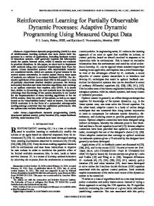
Figure 4. The environment. t u Now, we can give and prove the theorem that assures the convergence. Theorem 1 Let us consider the RL task associated to the BP F P given in Section 3. The BP F agent is trained using the algorithm indicated in Figure (2). If each state action pair is visited infinitely often during the training, then Qn (s, a) converges to Q∗ (s, a) as n → ∞, for all s, a. Using Lemmas 2 and 3, we have that the array Qn (s, a) increases and is upper bounded, which means that it is convergent. Moreover, it follows that the (superior) limit of Qn (s, a) is Q∗ (s, a). So, Theorem 1 is proven. t u

5

State

Action a1 = L

Action a2 = U

Action a3 = R

Action a4 = D

1 2 3 4 5 6 7 8 9 10 11 12 13 14 15 16 17 18 19 20 21 22

1.00000000

1.00000000

0.91900000

1.00000000

0.10900000 1.00000000

1.00000000 0.10900000

0.91000000 1.00000000

1.00000000 0.91000000

0.91000000

0.10900000

0.10000000

0.10900000

1.00000000

0.91000000

1.00000000

0.10900000

0.00000000 0.00000000

0.00000000 0.00000000

0.01000000 1.00000000

0.00000000 0.01000000

0.01000000 0.00000000

1.00000000 0.01000000

1.00000000 1.00000000

1.00000000 0.00000000

0.00000000

0.00000000

0.01000000

1.00000000

0.00000000

0.00000000

0.00000000

0.01000000

0.01000000

0.00000000

0.00000000

1.00000000

1.00000000 1.00000000

0.01000000 1.00000000

1.00000000 0.01000000

1.00000000 1.00000000

1.00000000 0.01000000

0.00000000 0.00000000

0.00000000 0.00000000

0.01000000 0.00000000

1.00000000

0.01000000

0.00000000

0.00000000

0.00000000

1.00000000

0.01000000

0.00000000

1.00000000 0.01000000 0.00000000 0.00000000

1.00000000 1.00000000 0.01000000 0.00000000

1.00000000 0.00000000 0.00000000 0.00000000

0.01000000 0.00000000 0.00000000 0.00000000

....... 85

....... 0.00000000

....... 0.00000000

....... 0.00000000

0.00000000

Table 1. The Q-values after traning was completed.

Computational experiments

In this section we aim at providing the reader with an easy to follow example illustrating how our approach works. Let us consider a HP protein sequence P = HHP H, consisting of four amino acids, i.e n = 4. As we have presented in Section 3, the states space will consist of 85 states, i.e S = {s1 , s2 , ..., s85 }. The states space is illustrated in Figure 4. In the figure the circles represent states and the transitions between states are indicated by arrows labeled with the action that leads the agent from a state to another.

5.1

Using the above defined parameters and under the assumptions that the state action pairs are equally visited during training and that the agent explores its search space (the  parameter is set to 1), the Q-values indicated in Table 1 were obtained. Three optimal solutions were reported after the training of the BF P agent was completed, determined starting from state s1 , following the Greedy policy (as we have indicated in Subsection 3). All these solutions correspond, having a minimum associated energy of −1. The optimal solutions are:

Experiment 1

First, we have trained the BP F agent as indicated in Subsection 3.2, using Formula (2) to update the Q-values estimates. We remark the following regarding the parameters setting: • the discount factor for the future rewards is γ = 0.9; • the number of training episodes is 36 training episodes; • the -Greeedy action selection mechanism was used;

1. The path π = (s1 s2 s7 s28 ) having the associated configuration aπ = (LU R) (Figure 5). 2. The path π = (s1 s3 s10 s41 ) having the associated configuration aπ = (U LD) (Figure 6). 3. The path π = (s1 s3 s12 s49 ) having the associated configuration aπ = (U RD) (Figure 7). 4. The path π = (s1 s5 s18 s71 ) having the associated configuration aπ = (DLU ) (Figure 8).

179

Gabriela Czibula,Maria Iuliona Bocicor,Istran Gergely Czibula, Int.J.Comp.Tech.Appl, 171-182

Figure 5. The con-

Figure 6. The con-

figuration learned is LU R. The value of the energy function for this configuration is −1.

figuration learned is U LD. The value of the energy function for this configuration is −1.

Figure 7. The con-

Figure 8. The con-

figuration learned is U RD. The value of the energy function for this configuration is −1.

figuration learned is DLU . The value of the energy function for this configuration is −1.

Consequently, the BP F agent learns a solution of the bidimensional protein folding problem, i.e a bidimensional structure of the protein P that has a minimum associated energy (−1).

5.2

Experiment 2

Secondly, we have trained the BP F agent as indicated in Subsection 3.2, but using for updating the Q-values estimates Formula (3). As proven in [21], the Q-learning algorithm converges to the real Q∗ -values as long as all state-action pairs are visited an infinite number of times, the learning rate α is small (e.q 0.01) and the policy converges in the limit to the Greedy policy. We remark the following regarding the parameters setting: • the learning rate is α = 0.01 in order to assure the convergence of the algorithm; • the discount factor for the future rewards is γ = 0.9; • the number of training episodes is 36 training episodes; • the -Greeedy action selection mechanism was used;

State

Action a1 = L

Action a2 = U

Action a3 = R

Action a4 = D

1

0.01532343

0.01521037

0.01530453

0.01531066

2 3

0.00394219 0.00420771

0.00412038 0.00394307

0.00066135 0.00420771

0.00411950 0.00066135

4

0.00066135

0.00394307

0.00394040

0.00394130

5

0.00403129

0.00057402

0.00403040

0.00394130

6 7

0.00000000 0.00000000

0.00000000 0.00000000

0.00010000 0.01000000

0.00000000 0.00010000

8 9

0.00010000 0.00000000

0.01000000 0.00010000

0.01000000 0.01000000

0.01000000 0.00000000

10

0.00000000

0.00000000

0.00010000

0.01000000

11

0.00000000

0.00000000

0.00000000

0.00010000

12

0.00010000

0.00000000

0.00000000

0.01000000

13 14

0.01000000 0.01000000

0.00010000 0.01000000

0.01000000 0.00010000

0.01000000 0.01000000

15 16

0.01000000 0.00010000

0.00000000 0.00000000

0.00000000 0.00000000

0.00010000 0.00000000

17

0.01000000

0.00010000

0.00000000

0.00000000

18

0.00000000

0.01000000

0.00010000

0.00000000

19 20 21 22

0.01000000 0.00010000 0.00000000 0.00000000

0.01000000 0.01000000 0.00010000 0.00000000

0.01000000 0.00000000 0.00000000 0.00000000

0.00010000 0.00000000 0.00000000 0.00000000

....... 85

....... 0.00000000

....... 0.00000000

....... 0.00000000

0.00000000

Table 2. The Q-values after traning was completed.

Using the above defined parameters and under the assumptions that the state action pairs are equally visited during training and that the agent explores its search space (the  parameter is set to 1), the Q-values indicated in Table 2 were obtained. The solution reported after the training of the BF P agent was completed is the path π = (s1 s2 s7 s28 ) having the associated configuration aπ = (LU R), determined starting from state s1 , following the Greedy policy (as we have indicated in Subsection 3). The solution learned by the agent is represented in Figure 9 and has an energy of −1. Consequently, the BP F agent learns the optimal solution of the bidimensional protein folding problem, i.e the bidimensional structure of the protein P that has a minimum associated energy (−1).

6

Disscussion

Regarding the Q-learning approach introduced in Section 3 for solving the bidimensional protein folding problem, we remark the following:

180

Gabriela Czibula,Maria Iuliona Bocicor,Istran Gergely Czibula, Int.J.Comp.Tech.Appl, 171-182

Figure 9. The learned solution is LU R. The value of the energy function for this configuration is −1.

• The training process during an episode has a time complexity of θ(n), where n is the length of the HP protein sequence. Consequently, assuming that the number of training episodes is k, the overall complexity of the algorithm for training the BP F agent is θ(k · n). • If the dimension n of the HP protein sequence is large and consequently the state space becomes very large n (consisting of 4 3−1 states), in order to store the Q values estimates, a neural network should be used. In the following we will briefly compare our approach with some of the existing approaches. The comparison is made considering the computational time complexity point of view. Since for the most of the existing approaches the authors do not provide the asymptotic analysis of the time complexity of the proposed approaches, we can not provide a detailed comparison. Hart and Belew show in [9] that an asymptotic analysis of the computational complexity for evolutionary algorithms (EAs) is difficult, and is done only for particular problems. He and Yao analyse in [10] the computational time complexity of evolutionary algorithms, showing that evolutionary approaches are computationally expensive. The authors give conditions under which EA need at least exponential computation time on average to solve a problem, which leads us to the conclusion that for particular problems the EA performance is poor. Anyway, a conclusion is that the number of generations (or equivalently the number of fitness evaluations) is the most important factor in determining the order of EA’s computation time. In our view, the time complexity of an evolutionary approach for solving the problem of predicting the structure of an n-dimensional protein is at least noOf Runs · n · noOf Generations · populationLength. Since our RL approach has a time complexity of θ(n · noOf Episodes), it is likely (even if we can not rigurously prove) that our approach has a lower computational complexity. Neumann et al. show in [13] how simple ACO algorithms can be analyzed with respect to their computational complexity on example functions with different prop-

erties, and also claim that asymptotic analysis for general ACO systems is difficult. In our view, the time complexity of an ACO approach for solving the problem of predicting th structure of an n-dimensional protein is at least noOf Runs · n · noOf Iterations · noOf Ants. Since our RL approach has a time complexity of θ(n · noOf Episodes), it is likely (even if we can not rigurously prove) that our approach has a lower computational complexity. Compared to the supervised classification approach from [7], the advantage of our RL model is that the learning process needs no external supervision, as in our approach the solution is learned from the rewards obtained by the agent during its training. It is well known that the main drawback of supervised learning models is that a set of inputs with their target outputs is required, and this can be a problem. We can conclude that a major advantage of the RL approach that we have introduced in this paper is the fact that the convergence of the Q-learning process was mathematically proven, and this confirms the potential of our proposal. We think that this direction of using reinforcement learning techniques in solving the protein folding problem is worth being studied and further improvements can lead to valuable results. The main drawback of our approach is that, as we have shown in Section 4, a very large number of training episodes has to be considered in order to obtain accurate results and this leads to a slow convergence. In order to speed up the convergence process, further improvements will be considered.

7

Conclusions and Further Work

We have proposed in this paper a reinforcement learning based model for solving the bidimensional protein folding problem. To our knowledge, except for the ant based approaches, the bidimensional protein folding problem has not been addressed in the literature using reinforcement learning, so far. The model proposed in this paper can be easily extended to solve the three-dimensional protein folding problem, and moreover to solve other optimization problems. We have emphasized the potential of our proposal by giving a mathematical validation of the proposed model, highlighting its advantages. We plan to extend the evaluation of the proposed RL model for some large HP protein sequences, to further test its performance. We will also investigate possible improvements of the RL model by analyzing a temporal difference approach [17], by using different reinforcement functions and by adding different local search mechanisms in order to increase the model’s performance. An extension of the

181

Gabriela Czibula,Maria Iuliona Bocicor,Istran Gergely Czibula, Int.J.Comp.Tech.Appl, 171-182

BP F model to a distributed RL approach will be also considered.

ACKNOWLEDGEMENT This work was supported by CNCSIS - UEFISCSU, project number PNII - IDEI 2286/2008.

References [1] C. B. Anfinsen. Principles that govern the folding of protein chains. Science, 181:223–230, 1973. [2] B. Berger and T. Leighton. Protein folding in hp model is np-complete. Journal of Computational Biology, 5:27–40, 1998. [3] T. Beutler and K. Dill. A fast conformational search strategy for finding low energy structures of model proteins. Protein Science, 5:2037–2043, 1996. [4] D. Chapman and L. P. Kaelbling. Input generalization in delayed reinforcement learning: an algorithm and performance comparisons. In Proceedings of the 12th international joint conference on Artificial intelligence - Volume 2, pages 726– 731, San Francisco, CA, USA, 1991. Morgan Kaufmann Publishers Inc. [5] C. Chira. Hill-climbing search in evolutionary models for protein folding simulations. Studia, LV:29–40, 2010. [6] K. Dill and K. Lau. A lattice statistical mechanics model of the conformational sequence spaces of proteins. Macromolecules, 22:3986–3997, 1989. [7] C. H. Q. Ding and I. Dubchak. Multi-class protein fold recognition using support vector machines and neural networks. Bioinformatics, 17:349–358, 2001. [8] M. Dorigo and T. St¨utzle. Ant Colony Optimization. Bradford Company, Scituate, MA, USA, 2004. [9] W. E. Hart and R. K. Belew. Optimizing an arbitrary function is hard for the genetic algorithm. In Proceedings of the Fourth International Conference on Genetic Algorithms, pages 190–195. Morgan Kaufmann, 1991. [10] J. He and X. Yao. Drift analysis and average time complexity of evolutionary algorithms. Artificial Intelligence, 127(1):57 – 85, 2001. [11] L. J. Lin. Self-improving reactive agents based on reinforcement learning, planning and teaching. Machine Learning, 8:293–321, 1992. [12] T. Mitchell. Machine Learning. New York: McGraw-Hill, 1997. [13] F. Neumann, D. Sudholt, and C. Witt. Computational complexity of ant colony optimization and its hybridization with local search. In Innovations in Swarm Intelligence, pages 91–120. 2009. [14] A. Perez-Uribe. Introduction to reinforcement learning, 1998. http://lslwww.epfl.ch/∼anperez/RL/RL.html. [15] S. Russell and P. Norvig. Artificial Intelligence - A Modern Approach. Prentice Hall International Series in Artificial Intelligence. Prentice Hall, 2003. [16] A. Shmygelska and H. Hoos. An ant colony optimisation algorithm for the 2d and 3d hydrophobic polar protein folding problem. BMC Bioinformatics, 6, 2005.

[17] R. S. Sutton and A. G. Barto. Reinforcement Learning: An Introduction. MIT Press, 1998. [18] T. Thalheim, D. Merkle, and M. Middendorf. Protein folding in the hp-model solved with a hybrid population based aco algorithm. IAENG International Jurnal of Computer Science, 35, 2008. [19] S. Thrun. The role of exploration in learning control. In Handbook for Intelligent Control: Neural, Fuzzy and Adaptive Approaches. Van Nostrand Reinhold, Florence, Kentucky, 1992. [20] R. Unger and J. Moult. Genetic algorithms for protein folding simulations. Mol. Biol., 231:75–81, 1993. [21] C. J. C. H. Watkins and P. Dayan. Q-learning. Machine Learning, 8(3-4):279–292, 1992. [22] X. Zhang, T. Wang, H. Luo, Y. Yang, Y. Deng, J. Tang, and M. Q. Yang. 3d protein structure prediction with genetic tabu search algorithm. BMC Systems Biology, 4, 2009.

182