A Relational Framework for Bounded Program Verification by
Gregory D. Dennis B.S., Massachusetts Institute of Technology (2002) M.Eng., Massachusetts Institute of Technology (2003) Submitted to the Department of Electrical Engineering and Computer Science in partial fulfillment of the requirements for the degree of Doctor of Philosophy in Computer Science and Engineering at the MASSACHUSETTS INSTITUTE OF TECHNOLOGY September 2009 c Massachusetts Institute of Technology 2009. All rights reserved.
Author . . . . . . . . . . . . . . . . . . . . . . . . . . . . . . . . . . . . . . . . . . . . . . . . . . . . . . . . . . . . . . Department of Electrical Engineering and Computer Science June 19, 2009 Certified by . . . . . . . . . . . . . . . . . . . . . . . . . . . . . . . . . . . . . . . . . . . . . . . . . . . . . . . . . . Daniel N. Jackson Professor Thesis Supervisor Accepted by . . . . . . . . . . . . . . . . . . . . . . . . . . . . . . . . . . . . . . . . . . . . . . . . . . . . . . . . . Professor Terry P. Orlando Chair, Department Committee on Graduate Students
2
A Relational Framework for Bounded Program Verification by Gregory D. Dennis Submitted to the Department of Electrical Engineering and Computer Science on June 19, 2009, in partial fulfillment of the requirements for the degree of Doctor of Philosophy in Computer Science and Engineering
Abstract All software verification techniques, from theorem proving to testing, share the common goal of establishing a program’s correctness with both (1) a high degree of confidence and (2) a low cost to the user, two criteria in tension with one another. Theorem proving offers the benefit of high confidence, but requires significant expertise and effort from the user. Testing, on the other hand, can be performed for little cost, but low-cost testing does not yield high confidence in a program’s correctness. Although many static analyses can quickly and with high confidence check a program’s conformance to a specification, they achieve these goals by sacrificing the expressiveness of the specification. To date, static analyses have been largely limited to the detection of shallow properties that apply to a very large class of programs, such as absence of array-bound errors and conformance to API usage conventions. Few static analyses are capable of checking strong specifications, specifications whose satisfaction relies upon the program’s precise behavior. This thesis presents a new program-analysis framework that allows a procedure in an object-oriented language to be automatically checked, with high confidence, against a strong specification of its behavior. The framework is based on an intermediate relational representation of code and an analysis that examines all executions of a procedure up to a bound on the size of the heap and the number of loop unrollings. If a counterexample is detected within the bound, it is reported to the user as a trace of the procedure, though defects outside the bound will be missed. Unlike testing, many static analyses are not equipped with coverage metrics to detect which program behaviors the analysis failed to exercise. Our framework, in contrast, includes such a metric. When no counterexamples are found, the metric can report how thoroughly the code was covered. This information can, in turn, help the user change the bound on the analysis or strengthen the specification to make subsequent analyses more comprehensive. Thesis Supervisor: Daniel N. Jackson Title: Professor
3
4
Acknowledgments Many people deserve my thanks and gratitude for making this thesis possible. First, a big thanks to my supervisor Daniel Jackson. It was Daniel’s teaching of 6.170 that ignited my interested in software design and development. After that class, I joined his Software Design Group as an undergraduate researcher, then a Masters student, and finally a Ph.D. Throughout that time, he has provided invaluable insights, challenges my assumptions, and made me think more deeply and clearly about every problem I encountered. Thanks, too, to the other members of my thesis committee: Carroll Morgan and Arvind. With their insights, edits, and tough questions, I was able to hone my thinking and clarify my presentation. During my time in SDG, I have had the pleasure of meeting and working with many smart people. First, a thanks to the doctoral students who welcomed me into the group when I first joined and provided mentorship and advice along the way: Sarfraz Khurshid, Ilya Shlyakhter, and Mandana Vaziri. I think, too, all the fellow students and researchers who joined about the same time I did and whom I relied upon for advice and laughs: Felix Chang, Jonathan Edwards, Carlos Pacheco, Derek Rayside, Robert Seater, Mana Taghdiri, and Emina Torlak. Finally, thanks to all the new additions to the group, whose energy and enthusiasm has been a source of inspiration: Zev Benjamin, Eunsuk Kang, Aleksandar Milicevic, Joe Near, Rishabh Singh, and Kuat Yessenov. Kuat deserves special thanks for his intense involvement building a Java front-end to my analysis. Without his tireless work understanding the Java Modelling Language and translating it to relational logic, the case studies would not have been possible. His more recent work on the JForge Eclipse plugin and specification language brought the usability and applicability of my research to an entirely new level. He has a bright future ahead. Finally, I thank my family. My parents, brothers, and sister were always there for me with encouragement and support. My mom’s warmth and my dad’s judgement are the backbones of my success. Most of all, I thank my loving wife Joselyn, who during my time as a Doctoral student, married me, bought a home with me, and gave birth to our beautiful son, Noah. She has always been patient and supportive, and Noah will soon realize how lucky he is to have a mother like her.
5
6
Contents 1 Introduction 1.1 The Cost vs Confidence Tradeoff 1.2 Strong vs Weak Specifications . . 1.3 Introducing Forge . . . . . . . . . 1.3.1 The Forge Framework . . 1.4 Forge from the User’s Perspective 1.4.1 An Example Analysis . . . 1.5 Discussion . . . . . . . . . . . . . 1.6 The Road Ahead . . . . . . . . .
. . . . . . . .
. . . . . . . .
. . . . . . . .
. . . . . . . .
. . . . . . . .
. . . . . . . .
. . . . . . . .
. . . . . . . .
. . . . . . . .
. . . . . . . .
. . . . . . . .
. . . . . . . .
. . . . . . . .
. . . . . . . .
. . . . . . . .
. . . . . . . .
. . . . . . . .
. . . . . . . .
. . . . . . . .
. . . . . . . .
15 15 16 17 18 20 23 25 26
2 Intermediate Representation 2.1 The FIR Grammar . . . . . . . 2.1.1 FIR expressions . . . . . 2.1.2 FIR Procedures . . . . . 2.2 Transforming FIR . . . . . . . . 2.2.1 Unrolling Loops . . . . . 2.2.2 Inlining Procedure Calls 2.3 Chapter Summary . . . . . . .
. . . . . . .
. . . . . . .
. . . . . . .
. . . . . . .
. . . . . . .
. . . . . . .
. . . . . . .
. . . . . . .
. . . . . . .
. . . . . . .
. . . . . . .
. . . . . . .
. . . . . . .
. . . . . . .
. . . . . . .
. . . . . . .
. . . . . . .
. . . . . . .
. . . . . . .
. . . . . . .
27 28 30 33 36 37 39 40
3 Bounded Verification 3.1 Model Finding with Relational Logic . . . . 3.1.1 Using Kodkod . . . . . . . . . . . . . 3.2 Symbolic Execution . . . . . . . . . . . . . . 3.2.1 Small Example: Social Network . . . 3.2.2 Building the Initial State . . . . . . . 3.2.3 Translating Expressions . . . . . . . 3.2.4 Formal Execution Rules . . . . . . . 3.2.5 Generating the Logic Problem . . . . 3.2.6 Larger Example: Web Registration . 3.3 A Correctness Argument . . . . . . . . . . . 3.3.1 Semantics . . . . . . . . . . . . . . . 3.3.2 Symbolic Execution . . . . . . . . . . 3.3.3 Proof Framework . . . . . . . . . . . 3.3.4 Applying the Proof System to Forge 3.3.5 Summary of Correctness Argument .
. . . . . . . . . . . . . . .
. . . . . . . . . . . . . . .
. . . . . . . . . . . . . . .
. . . . . . . . . . . . . . .
. . . . . . . . . . . . . . .
. . . . . . . . . . . . . . .
. . . . . . . . . . . . . . .
. . . . . . . . . . . . . . .
. . . . . . . . . . . . . . .
. . . . . . . . . . . . . . .
. . . . . . . . . . . . . . .
. . . . . . . . . . . . . . .
. . . . . . . . . . . . . . .
. . . . . . . . . . . . . . .
41 42 42 45 45 49 49 52 56 56 64 64 65 65 66 71
. . . . . . .
7
3.4
Breaking Symmetries on Dynamic Allocation . 3.4.1 Isomorphic Allocation Orders . . . . . 3.4.2 Modified Initial State . . . . . . . . . . 3.4.3 Modified Rules for Create Statements. 3.4.4 Implications for Correctness . . . . . . 3.5 Chapter Summary . . . . . . . . . . . . . . .
. . . . . .
. . . . . .
. . . . . .
. . . . . .
. . . . . .
. . . . . .
. . . . . .
. . . . . .
. . . . . .
. . . . . .
. . . . . .
. . . . . .
. . . . . .
71 72 73 74 75 76
4 Coverage Metric 4.1 Examples of Poor Coverage . . . . . . . . . . . . . . 4.2 Exploiting the Unsatisfiable Core . . . . . . . . . . . 4.3 Symbolic Execution with Formula Slicing . . . . . . . 4.3.1 Example: Coverage of the Register Procedure 4.3.2 The Problem with the Inline Strategy . . . . . 4.4 Coverage before Unrolling . . . . . . . . . . . . . . . 4.5 Chapter Summary . . . . . . . . . . . . . . . . . . .
. . . . . . .
. . . . . . .
. . . . . . .
. . . . . . .
. . . . . . .
. . . . . . .
. . . . . . .
. . . . . . .
. . . . . . .
77 77 80 81 82 83 84 86
5 Object Orientation and Data Abstraction 5.1 From Object-Oriented Code to FIR . . . . . . . . . . . . 5.1.1 An Example Translation . . . . . . . . . . . . . . 5.1.2 Complexities of Real Programs . . . . . . . . . . 5.1.3 Unsoundness and Incompleteness . . . . . . . . . 5.2 Dealing with Abstraction . . . . . . . . . . . . . . . . . . 5.2.1 Abstraction Function & Representation Invariant 5.2.2 Invariant Preservation and Trace Inclusion . . . .
. . . . . . .
. . . . . . .
. . . . . . .
. . . . . . .
. . . . . . .
. . . . . . .
. . . . . . .
87 87 88 90 91 92 93 94
. . . . . . . . . . . . . .
97 97 97 99 100 100 102 103 105 106 108 109 112 113 114
6 Case Studies 6.1 Case Study 1: Linked Lists . . . . . . . . . . . . . . . 6.1.1 Results . . . . . . . . . . . . . . . . . . . . . . 6.1.2 Scope Effects . . . . . . . . . . . . . . . . . . 6.1.3 Specification Errors . . . . . . . . . . . . . . . 6.2 Case Study 2: Electronic Voting Software . . . . . . . 6.2.1 Specification Violations . . . . . . . . . . . . . 6.2.2 Example Violations . . . . . . . . . . . . . . . 6.2.3 Why were these problems missed? . . . . . . . 6.3 Case Study 3: Strategy/Coverage Evaluation . . . . . 6.3.1 Performance of Symbolic Execution Strategies 6.3.2 Mutant Generation . . . . . . . . . . . . . . . 6.3.3 Infinite Loop Detection . . . . . . . . . . . . . 6.3.4 Insufficient Bound Detection . . . . . . . . . . 6.4 Chapter Summary . . . . . . . . . . . . . . . . . . .
. . . . . . . . . . . . . .
. . . . . . . . . . . . . .
. . . . . . . . . . . . . .
. . . . . . . . . . . . . .
. . . . . . . . . . . . . .
. . . . . . . . . . . . . .
. . . . . . . . . . . . . .
. . . . . . . . . . . . . .
7 Discussion 115 7.1 Verification with Relational Logic . . . . . . . . . . . . . . . . . . . . 115 7.1.1 Jalloy . . . . . . . . . . . . . . . . . . . . . . . . . . . . . . . 115 8
7.2
7.3
7.4
7.5
7.1.2 Karun . . . . . . . . . . . . . . . . . 7.1.3 Verification with DynAlloy . . . . . . Related Languages & Representations . . . . 7.2.1 Relational Programming Languages . 7.2.2 Intermediate Representations . . . . Related Program Analyses . . . . . . . . . . 7.3.1 Testing . . . . . . . . . . . . . . . . . 7.3.2 Theorem Proving . . . . . . . . . . . 7.3.3 Model Checking . . . . . . . . . . . . 7.3.4 Shape Analysis . . . . . . . . . . . . Related Coverage Metrics . . . . . . . . . . 7.4.1 Coverage Metrics for Testing . . . . . 7.4.2 Coverage Metrics for Model Checking 7.4.3 A Coverage Metric for ESC? . . . . . Conclusions . . . . . . . . . . . . . . . . . .
9
. . . . . . . . . . . . . . .
. . . . . . . . . . . . . . .
. . . . . . . . . . . . . . .
. . . . . . . . . . . . . . .
. . . . . . . . . . . . . . .
. . . . . . . . . . . . . . .
. . . . . . . . . . . . . . .
. . . . . . . . . . . . . . .
. . . . . . . . . . . . . . .
. . . . . . . . . . . . . . .
. . . . . . . . . . . . . . .
. . . . . . . . . . . . . . .
. . . . . . . . . . . . . . .
. . . . . . . . . . . . . . .
116 118 118 118 118 119 120 122 123 126 126 127 127 127 128
10
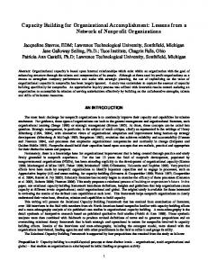
List of Figures 1-1 Cost vs. Confidence comparison of testing and theorem proving. . . . 1-2 The Forge Tradeoff. Forge is economical for those development projects spending anywhere in the gray area on testing. For that cost, Forge offers greater confidence, and for that level of confidence, Forge could offer a lower cost. . . . . . . . . . . . . . . . . . . . . . . . . . . . . . 1-3 The Forge Framework. Elements in black are the contributions of this thesis; gray are the contributions of others; and white have yet to be developed. . . . . . . . . . . . . . . . . . . . . . . . . . . . . . . . . . 1-4 Linked List Implementation & Specification . . . . . . . . . . . . . . 1-5 The get method and its counterexample trace. . . . . . . . . . . . . .
16
2-1 FIR Grammar . . . . . . . . . . . . . . . . . . . . . . . . . . . . . . . 2-2 Website Registration Program in FIR . . . . . . . . . . . . . . . . . . 2-3 Three Examples of Relational Join. For each tuple in p of the form hp1 , . . ., pn , mi and tuple in q of the form hm, q1 , . . ., qk i, there is a tuple in p.q of the form hp1 , . . ., pn , q1 , . . ., qk i. Example (ii): when p is a set, the join p.q is equivalent to the relational image of q under p. Example (iii): when p is a singleton and q is a function, p.q is equivalent to function application. . . . . . . . . . . . . . . . . . . . . 2-4 List containment procedure in FIR . . . . . . . . . . . . . . . . . . . 2-5 The contains procedure unrolled twice. Gotos indicate aliased statements. The thickness of the lines is used only to disambiguate line crossings. . . . . . . . . . . . . . . . . . . . . . . . . . . . . . . . . .
28 29
3-1 Relational Logic . . . . . . . . . . . . . . . . . . . . . . . . . . . . . . 3-2 Semantics of FIR Expression Translation . . . . . . . . . . . . . . . . 3-3 Symbolic Execution Rules. For assign, create, and branch statements, the “inline” rule (=⇒I ) or the “constrain” rule (=⇒C ) may be applied. All primed relational variables, e.g. v 0 , are fresh. . . . . . . . . . . . . 3-4 Website registration procedure in FIR . . . . . . . . . . . . . . . . . .
43 51
4-1 Examples of Poor Coverage. Bounded verification does not find counterexample for these examples, yet problems remain. The statements shown in gray are “missed” (not covered) by the bounded verification analysis. . . . . . . . . . . . . . . . . . . . . . . . . . . . . . . . . . . 4-2 Register procedure . . . . . . . . . . . . . . . . . . . . . . . . . . . . 11
18
19 22 24
30 38
38
53 57
78 82
5-1 Birthday Example in Java . . . . . . . . . . . . . . . . . . . . . . . . 5-2 Translation of Birthday.setDay into FIR . . . . . . . . . . . . . . .
89 89
6-1 Strategy Performance Comparison. The bars show the average number of variables, clauses, and time-to-solve for the SAT problems generated by each strategy, as a factor of those numbers for the “aI cI bI” strategy.109 6-2 Percentage of Mutants Killed per Bound. A bound of n is a scope of n, bitwidth of n, and n loop unrollings. . . . . . . . . . . . . . . . . . 111
12
List of Tables 6.1 6.2
6.3 6.4 6.5 6.6
6.7
6.8
Duration of Method Analyses (seconds) . . . . . . . . . . . . . . . . . Summary analysis statistics of each class. Means are calculated over the analyses of the methods within a class, not over successive analyses of the same class. . . . . . . . . . . . . . . . . . . . . . . . . . . . . . Specification violations: error classification and minimum bound (scope / bitwidth / unrollings) necessary for the error’s detection. . . . . . . Characteristics of the benchmark problems. . . . . . . . . . . . . . . MuJava Mutation Operators . . . . . . . . . . . . . . . . . . . . . . . Mutants per Benchmark and Minimal Bound for Detection of All Killable Mutants. A mutant is not killable by bounded verification if it is equivalent to the original method on all of its terminating executions. A bound of “sS bB uU ” is a scope of S on each type, a bitwidth of B, and U loop unrollings . . . . . . . . . . . . . . . . . . . . . . . . . . . Infinite Loop Detection. The “missed” column lists the number of missed statements measured in an infinitely-looping mutant compared to the original method. . . . . . . . . . . . . . . . . . . . . . . . . . . Insufficient Bound Detection. . . . . . . . . . . . . . . . . . . . . . .
13
98
101 102 107 110
111
112 114
14
Chapter 1 Introduction Software failures continue to pose a major problem to software development and the economy generally. Studies have estimated software errors to account for between 25% and 35% of system downtime [76, 71]. A 2002 study by the National Institute of Standards & Technology (NIST) estimated the annual cost of software failures in the U.S. at between $20 and $60 billion [68], or as much as 0.6% of the U.S. GDP. The consequences of these failures vary greatly, from the merely annoying, such as the crash of a desktop word processor, to the tragic, such as the 28 overdoses delivered by a radiotherapy machine in Panama City in 2001, an event which led to 17 deaths [44]. Software verification techniques hold the promise of dramatically reducing the number of defects in software. The term “software verification” refers here to all manner of checking program correctness: from formal verification approaches like theorem proving, to dynamic analyses like testing, to static analyses, such as ESC/Java. Ideally, these techniques would establish that a program is correct with a high degree of confidence while requiring limited cost from the user, but these two goals — high confidence and low cost — are at odds. Theorem proving, for example, offers the benefit of high confidence, but requires significant expertise and effort from the user. Testing, on the other hand, can be performed for little cost, but low-cost testing does not yield high confidence in a program’s correctness.
1.1
The Cost vs Confidence Tradeoff
Our assessment of the cost-versus-confidence tradeoff of testing and theorem proving is shown in Figure 1-1. “Cost” in the figure refers to both the time required to carry out the technique and the cost of employing someone with the expertise to carry it out. “Confidence” refers to the degree of certainty in the program’s correctness that the analysis provides. Due to its low initial costs, testing can be an attractive option for checking program correctness. A handful of test cases can be written quickly without much expertise, run fully automatically, and when bugs are found, testing provides the user with concrete counterexample traces that exhibit the error. As shown in Figure 1-1, testing allows users, for relatively little cost, to obtain an immediate boost of confidence in the correctness of their code. 15
confdence
testing theorem proving
cost Figure 1-1: Cost vs. Confidence comparison of testing and theorem proving.
The challenge of testing is that high confidence is very difficult and costly to obtain. Test selection, test generation, and calculation of coverage metrics are tasks too tedious to be performed manually, and building testing infrastructure to automate them causes dramatic increases in cost. As a result, the testing curve in Figure 1-1 quickly levels off. The eventual high costs of testing explain why it consumes about half the total cost of all software development [11] and why Microsoft, for example, employs approximately one tester for every developer [17]. If very high confidence is required, a developer might instead opt for theorem proving. As its name implies, theorem proving yields a proof of the program’s correctness — a very high level of confidence. However, as reflected in Figure 1-1, theorem proving requires a large investment in both time and expertise before any confidence is obtained. It is common for a theorem prover to carry a learning curve of about 6 months, even for a highly skilled software developer [87, 6]. That amount of upfront investment makes theorem proving prohibitively expensive for most projects.
1.2
Strong vs Weak Specifications
One area with much recent progress in combining high confidence with low cost is static analysis. A variety of static-analysis tools can now automatically check a program for conformance to a specification and provide a high degree of confidence in their result. Some of these tools, like FindBugs [2], use pattern-based heuristics; others, such as Astr´ee [1], use abstract interpretation; some combine abstract interpretation and model checking, like SLAM [8]; and others are explicit-state model checkers, like SPIN [43].
16
However, these analyses, by and large, achieve their combination of full automation and high confidence by sacrificing the expressiveness of the specifications they accept. To date, static analyses have largely been limited to checking code against very partial properties that apply to a large class of programs, such as the absence of array-bound errors and conformance to API usage conventions. Some shape analyses, like SATC [42], can check deeper, structural properties of the heap, such as list acyclicity, but these are nevertheless still very partial correctness properties. Less progress has been made in static analyses for checking strong specifications. A “strong specification” here refers to a detailed property that is specific to the individual program under analysis.1 For the software controlling a radiotherapy machine, a strong specification may be that “the radiotherapy machine delivers the prescribed dose,” and for a voting system perhaps “the winner of the election has the most votes.” These are properties that require the precise behavior of the code for their satisfaction, and thus cannot be analyzed by a technique that relies on abstraction, a technique common to static analysis generally. Strong specifications are typically written by the user in a general-purpose specification language, such as Larch [41], the Java Modeling Language [58], or Spec# [10]. To summarize, while many static analyses deliver high confidence at a low cost, they typically do so with respect to a partial, general-purpose property, not a strong, program-specific specification. As a result, the high confidence they offer in the program’s correctness with respect to that property does not translate into high confidence in its correctness overall.
1.3
Introducing Forge
While there is much research dedicated to shifting the testing curve in Figure 1-1 up (to increase its confidence) and other research to shift the theorem proving curve to the left (to lower its cost), the analysis presented in the this thesis, implemented in a tool called Forge, aims for a different cost/confidence tradeoff. As illustrated in Figure 1-2, it requires a greater upfront investment than testing, but once that initial investment is made, it provides a dramatic increase in confidence. Being fully automatic, its cost is much lower than theorem proving, though it can never attain the confidence of a proof. And unlike most automatic static analyses, which sacrifice the expressiveness of the specifications they accept, Forge is capable of checking a procedure against a strong, user-provided property of its behavior. We expect Forge to be economical for those software projects whose current investment falls somewhere in the gray area in Figure 1-2 but are currently situated on the testing curve. The black circle in the figure is example of where those projects might currently lie, and the arrows point to where they might move in the space if they were to adopt Forge. For their current level of investment, Forge could significantly increase the level of confidence in the software’s correctness. Or, if the current level of confidence is already deemed adequate, Forge could obtain that confidence for lower cost. 1
The term “strong specification” is borrowed from Robby, Rodr´ıguez, Dwyer, and Hatcliff [72]
17
confdence
Forge
testing theorem proving
cost Figure 1-2: The Forge Tradeoff. Forge is economical for those development projects spending anywhere in the gray area on testing. For that cost, Forge offers greater confidence, and for that level of confidence, Forge could offer a lower cost.
1.3.1
The Forge Framework
Forge is a program-analysis framework that allows a procedure in a conventional object-oriented language to be checked against a strong specification of its behavior. The Forge framework is shown in Figure 1-3. The elements in black in the framework are the contributions of this thesis; elements in the gray are the contributions of others; and those in white have yet to be developed.2 At the center of the framework sits the Forge tool. Forge accepts as input a procedure, a specification of the procedure, and a bound on the analysis. The procedure and its specification are both expressed in the Forge Intermediate Representation, or FIR. Discussed in greater detail in Chapter 2, FIR is a simple relational programming language that is amenable to analysis. FIR is intended to be produced by a mechanical translation from a conventional high-level programming language, but a user could also program in FIR directly. Specifications in FIR can involve arbitrary first-order logic, plus a relational calculus that includes transitive closure. The bound provided to Forge consists of the following: • a number of times to unroll each loop and recursive call; • a bitwidth limiting the range of FIR integers; and • a scope for each type, i.e., a limit on the number of its instances that may exist in any heap reached during execution.
2
JForge was a collaborative effort with Kuat Yessenov.
18
java method
fr procedure
java spec
fr spec
P(t,t') P ^ ¬S
java bound
jforge
fr bound
S(t,t')
forge
bound
kodkod
java trace
fr trace
solution
java coverage
fr coverage
unsat core
Figure 1-3: The Forge Framework. Elements in black are the contributions of this thesis; gray are the contributions of others; and white have yet to be developed. Forge searches exhaustively within this bound for a trace of the procedure that violates the specification. Bugs outside the bound will be missed, but in exchange for that compromise, the analysis is fully automated and delivers concrete counterexamples. The success of this bounded verification approach rests on an idea called the “small-scope hypothesis,” which is the expectation that bugs will usually have small examples. It’s a hypothesis consistent with our own experience, with prior empirical evaluation [5, 27, 28], and with the case studies presented in Chapter 6 of this thesis. To perform the exhaustive search, Forge encodes the FIR procedure and specification in the relational logic accepted by the Kodkod model finder [84]. From the procedure, Forge automatically obtains a formula P (s, s 0 ) in this logic that constrains the relationship between a pre-state s and a post-state s 0 that holds whenever an execution exists from s that terminates in s 0 . The states are vectors of free relational variables declared in the logic. The translation of the procedure to the logic uses a symbolic execution technique presented in Chapter 3. A second formula ψ(s, s 0 ) is obtained from the provided specification, the negation of which is conjoined to P yielding the following formula, which is true exactly for those executions that are possible but that violate the specification. P (s, s0 ) ∧ ¬ψ(s, s0 )
(1.1)
This formula is equivalent to the negation of (P (s, s 0 ) ⇒ ψ(s, s 0 )), the claim that every execution of the procedure satisfies the specification. Forge translates the bound on the FIR procedure into a bound on the relations in states s and s 0 and hands the formula and resulting bound to Kodkod. Using a SAT solver, Kodkod exhaustively searches for a solution to the formula within the bound, and reports such a solution if one exists. Forge then translates this solution back into a counterexample trace of the FIR procedure. 19
Since bounded verification is unsound, when no counterexamples are found it is unclear how much confidence one should have that the procedure meets its specification. For example, was the bound on the analysis too small to fully exercise all of the procedure’s behaviors? Testing addresses this problem with coverage metrics, analyses which can reveal behaviors of code that a test suite has left unexplored, but most static analyses offer nothing analogous. Forge includes its own coverage metric, analogous to those for testing, which, in the absence of counterexamples, can identify a subset of the code that was not explored. This information can, in turn, inform the user how to tune Forge to attain a more comprehensive analysis. The coverage metric, which is based on an “unsatisfiable core” formula reported by Kodkod, is explained in detail in Chapter 4. Since Forge operates on code and specifications written in the intermediate representation, analyzing a conventional high-level language requires a front-end for translating that language and its specifications to FIR. The Forge framework includes JForge, a front-end tool for translating Java code and specifications written in the JForge Specification Language [90] into FIR. A front-end for C is being developed independently by Toshiba Research [75]. Chapter 5 explains how a high-level objectoriented programming language like Java is translated to FIR. As will be explained, there are some limitations in this translation: it cannot handle some features of Java, including multithreading and real numbers, and it uses a few unsound optimizations that can theoretically lead to false alarms (Section 5.1.3). It is left to future work on JForge to map the trace and coverage information produced by Forge back to the original Java code. When analyzing object-oriented programs, an additional complexity arises from the specification of abstract data types. Note that in Formula 1.1, the procedure and specification are formulas over the same state, but when checking a procedure of an abstract data type, the (abstract) representation referred to in the specification usually differs from the (concrete) representation in the code. Chapter 5 addresses how to make such specifications amenable to the bounded verification analysis. We have conducted a series of case studies with Forge demonstrating its utility and feasibility, and these are presented in Chapter 6. Finally, related work, directions for future work, and general conclusions are discussed in Chapter 7. But before embarking on these technical presentations, the following section demonstrate how the Forge framework looks from the user’s perspective.
1.4
Forge from the User’s Perspective
This section illustrates a user’s experience with the Forge framework on a small example. The example involves checking a method of a linked-list implementation against its specification. The code and specification of the linked list is shown in Figure 1-4. The linked list is circular and doubly-linked, and for simplicity, the buckets in the list are themselves the values3 . Clients of the list are expected to extend the abstract Value class with the values they wish to store in the list. 3
The implementation is similar to the TLinkedList class provided by the GNU Trove library [3].
20
In this example, our hypothetical user wishes to check the get method of the linked list against its specification. A bug has deliberately been seeded in the get method: in the body of the first for-loop, value should be assigned value.next instead of value.prev. Because this bug does not raise a runtime error, tools that search for shallow properties like the absence of null pointer dereferences and array out-of-bounds errors cannot catch it. To detect the bug, one must apply an analysis that is capable of checking a code against a strong specification of its behavior. The strong specifications found in Figure 1-4 have been written by our user in the JForge Specification Language (JFSL)4 [90]. JFSL is not a contribution of this thesis and so will not be discussed in depth, but enough will be explained to understand this example. JFSL specifications are written in the form of Java annotations, which are special Java metadata constructs that begin with the ‘@’ symbol. The SpecField annotation at the top of Figure 1-4 declares a specification field named elems that serves as the abstract representation of the list data type. The elems field is of type seq Value, meaning it is a sequence of Value objects. In JFSL, a sequence declared of type seq T is actually a binary relation mapping integers to elements drawn from type T, whose domain is constrained to consist of consecutive integers, starting at zero. So elems, while conceptually a sequence, is semantically a binary relation of type Integer → Value. For example, the sequence [A, B, C] would be encoded in elems as the binary relation {h0,Ai, h1,Bi, h2,Ci}. The formula given in a SpecField annotation is the abstraction function that determines the value of the specification field from the values of the concrete fields. The abstraction function in Figure 1-4 gives an inductive definition of elems as a conjunction of two constraints. According to the first constraint (the base case of the induction), the first element in the sequence equals the set-difference of the head field and null. When head is null, there is no first element (this.elems[0] is the empty set); and when head is not null, the first element equals head. The second constraint (the inductive case) says that for every positive integer i, the element at index i in the sequence equals the next field of the element at index (i - 1), unless next equals head, which indicates the end of the list has been reached. The representation invariant of LinkList is given by the Invariant annotation, where it is expressed as two (implicitly conjoined) constraints. According to the first constraint, when the head field is not null, the head is reachable from itself by following the next field one or more times. The expression ^next denotes the transitive closure of the next field. The second constraint says the size field is equal to the number of reachable values in the list. The ‘#’ symbol is the cardinality operator: #e yields the number of tuples in the relation e. The specification of the get method is expressed in three annotations on the method: Requires, Returns, and Throws. The Requires annotation specifies a precondition under which no exception is thrown, in this case it is that the index argument is within the bounds of the list, i.e., it is non-negative and less than the length of the list. The expression #this.elems yields the number of tuples in the sequence, which is the same as the length of the sequence. The Returns annotation 4
JFSL is a product of ongoing work led by Kuat Yessenov.
21
@SpecField("elems: seq Value | " + "(this.elems[0] = this.head - null) && " + "(all i: int | i > 0 => this.elems[i] = this.elems[i-1].next - this.head)") public class LinkList { @Invariant({"this.head != null => this.head in this.head.^next", "#this.head.^next = this.size"}) private Value head; private int size; @Requires("index >= 0 && index < #this.elems") @Returns("this.elems[index]") @Throws("IndexOutOfBoundsException: index < 0 || index >= #this.elems") public Value get(int index) { // check whether index is in bounds checkIndex(index); Value value; // if index is in front half of list, // search from the first element if (index < (size >> 1)) { value = head; for (int i = 0; i < index; i++) { value = value.prev; } } // if index is in back half of list, // search from the second-to-last value else { value = head.prev; for (int i = size - 1; i > index; i--) { value = value.prev; } } return value; } @Requires("index >= 0 && index < #this.elems") @Throws("IndexOutOfBoundsException: index < 0 || index >= #this.elems") private void checkIndex(int index) { if (index < 0 || index >= size) { throw new IndexOutOfBoundsException(); } } @Invariant("next = ~prev") public static abstract class Value { Value next, prev; } }
Figure 1-4: Linked List Implementation & Specification 22
specifies an expression to be returned by the method when the precondition given by Requires is true. The expression in the Returns annotation, this.elems[index], evaluates to the Value at the given index in the elems sequence. The Throws annotation specifies that the method throw an IndexOutOfBoundsException when index is out of bounds. The specification of checkIndex has the same Requires and Throws annotations as the specification of get, because it throws the same exception under the same conditions. Lastly, the inner class Value has an invariant that the next field is the relational transpose (∼) of the prev field. In other words, if following the next field of x yields y, then following the prev field of y must yield x. Code that is not relevant to the analysis of the get method is not shown in Figure 1-4.
1.4.1
An Example Analysis
To perform an analysis with Forge, the user provides a bound on the analysis, consisting of a number of loop unrollings, a bitwidth to restrict the range of integers, and a scope on each type. The “scope” of a type is a limit on the number of instances of that type that may exist over the course of an execution. For this example, our hypothetical user applies JForge to analyze the get method initially in a scope of 3 Value instances and 1 LinkList, a bitwidth of 4, and 1 loop unrolling. The analysis completes in about two seconds and reports that “no counterexamples were found.” Not sufficiently confident that no bugs exist, our user invokes Forge’s coverage metric, which responds by highlighting statements that were missed (not covered) by the prior analysis. A statement is “missed” if the analysis would have still succeeded had been removed from the procedure. For our example analysis, the coverage metric highlights the first for-loop as missed:5 : . . . if (index < (size >> 1)) { value = head; for (int i = 0; i < index; i++ ) { value = value.prev; } } . . . From this coverage information, our user realizes that her chosen bound of 3 Value instances was too small for adequate coverage, because the first for-loop is unnecessary for lists of length 3 or less. If the list is of length 3, then index arguments equal to 1 or 2 are reached from traversing from the end of the list. Only an index of 0 is reached by iterating from the front-half of the list, and when the for-loop is reached with an index of 0, the loop condition is immediately false, rendering the entire loop unnecessary. 5
The metric highlights statements in FIR code but is not yet mapped to Java source code.
23
public Value get(int index) { checkIndex(index); Value value; if (index < (size >> 1)) { value = head; for (int i = 0; i < index; i++) { value = value.prev; } } else { value = head.prev; for (int i = size - 1; i > index; i--) { value = value.prev; } } return value; }
initial state: LinkList = {L0} Value = {V0, V1, V2, V3} this = L0 index = 1 elems = {, , , } head = {} next = {, , , } prev = {, , , } size = {} checkIndex(index): if (index < (size >> 1)): true value = head: value = V0 int i = 0: i = 0 i < index: true value = value.prev: value = V3 i++: i = 1 i < index: false return value: return = V3
Figure 1-5: The get method and its counterexample trace.
24
Desiring a more thorough analysis, our user increases the scope of Value to four instances and runs Forge again. The analysis again completes in two seconds, but this time finds a trace of the get method that violates its specification. This trace is shown in Figure 1-5. This trace is an execution of the get method where the index argument is 1 and the list is the sequence [V0, V1, V2, V3]. The return value should therefore be V1, but it is incorrectly V3. By inspecting the trace, the user discovers the error (value is assigned value.prev in the first loop instead of value.next). After fixing the error, the user repeats the Forge analysis and it reports that counterexamples are no longer found. However, the tool still shows some statements missed by the analysis. The user increases the scope to 5 and then finally to 6 Value instances, at which point the analysis completes in two minutes and reports full coverage. (The analysis time when coverage mode is turned off is 10 seconds.) Although the analysis has reached full coverage and no counterexamples are found, it has not established a proof of correctness. Full coverage indicates only that the coverage analysis has reached the limit of its ability to discover areas where bugs may exist.
1.5
Discussion
The linked list example makes concrete several of the features and characteristics of the Forge framework. First and foremost, it demonstrates the ability of Forge to check a method in an object-oriented program against a strong specification of its behavior. Even many tools that ostensibly check strong specifications, such as ESC/Java2 [23], would not be able to handle the specification in this example, because it used transitive closure, a feature which they do not support. The example showcased some advantages of Forge over theorem provers. Once the bound was chosen, the analysis was fully automatic and did not require user interaction or the writing of loop invariants as required by verification techniques, like Boogie [9] for example. Also, the code failures are presented as counterexample traces, rather than failed verification conditions or open subgoals that theorem provers often report. The traces make locating the error a relatively easy task. A test suite that achieves full branch coverage would have probably found the bug, but not necessarily. Indeed, if the sequence has duplicates, then with the right argument, the method could return the correct value even when a test case branches into the first for-loop to execute the erroneous statement. Although that is unlikely, the observation highlights the fact that a test suite that achieves full branch or path coverage makes no claim about which heap configurations have been explored. Bounded verification, in contrast, makes a specific claim about the heaps explored — all those within the user-provided bound — and when combined with the coverage metric illustrated, makes a claim about code coverage as well. 25
The initial analysis in a scope of three value instances and of 4 explored Pa7 bitwidth k all lists up to length 7 with 3 unique elements. There are k=0 3 = 3280 such lists and and 16 different integer arguments, for a total of 16 × 3280 = 52, 480 argument combinations explored, a large number of test cases to write and execute. With Forge, all those tests were effectively constructed and simulated in two The final P7seconds. k analysis in a scope of 6 values explored the equivalent of 16 × k=0 6 = 5, 374, 768 tests and the analysis completes in 10 seconds. Granted, many of those lists are isomorphic to one another; by our calculation there are 1155 non-isomorphic lists up to length 7 for a total of 18480 test cases. But avoiding non-isomorphic tests in general would pose an additional burden on a tester. Forge is able to avoid searching through many isomorphic structures for free by relying on the symmetry breaking capabilities of the underlying Kodkod model finder. Forge’s bounded verification analysis is unsound: when it does not find a trace of the procedure that violates the specification, that is not a guarantee of the program’s correctness. However, the coverage analysis helps mitigate that unsoundness. In our example, coverage reported by Forge showed that the initial analysis had not exercised the statement inside the first for-loop, which motivated our hypothetical user to expand the bound, thereby leading to the bug’s detection.
1.6
The Road Ahead
The remainder of the thesis describes the techniques that make this user experience possible. It covers the following topics: • the intermediate representation on which the Forge analyses are performed; • the bounded verification analysis that given a procedure and specification in the intermediate representation searches for a trace of the procedure that violates the specification; • the coverage metric that reports how thoroughly the bounded verification analysis examined the code; • techniques for applying the Forge analysis to programs written in high-level languages; • case studies in which Forge was used to analyze Java programs; and • discussion of related work, suggestions for future directions, and general reflections on the tool. Enjoy!
26
Chapter 2 Intermediate Representation Due to the complexities of dealing with high-level programming languages, many program verification techniques encode high-level programs in an intermediate representation (IR) that is more amenable to analysis [59]. ESC/Java [37] and ESC/Java2 [23] encode Java in a variant of Dijkstra’s guarded commands [31]; Boogie [9] encodes .NET bytecode in BoogiePL [25]; the Bogor model checker [72] encodes Java in the Bandera Intermediate Representation [46]; and Krakatoa [62] and Caduceus [36] encode Java and C, respectively, into the Why language [35]. These intermediate representations facilitate transformations and optimizations of the code, and they simplify the eventual translation to verification conditions. The Forge Intermediate Representation (FIR) is the language on which the Forge bounded verification and coverage analyses are performed. In contrast to other intermediate representations, FIR is relational. That is, every expression in the language evaluates to a relation, a feature that makes its semantics simple and uniform, and therefore, more amenable to automatic analysis. In addition to being a programming language, FIR is at the same time a specification language. As will be illustrated in this chapter, declarative specification can be embedded as statements — specification statements — within what is otherwise imperative code. And FIR expressions can include arbitrary first-order logic (any alternation of quantifiers), a useful, if not necessary, feature for writing strong specifications. Modeling code and specifications with a combination of first-order logic and a relational calculus is an idea drawn from experience with the Alloy modeling language [48] and the Kodkod model finder [84]. User experience with Alloy has shown that a combination of first-order and relational logic can encode the heap of an object program and operations on that heap in a clear and concise way [47]. Further experience and empirical data [82] has demonstrated the Kodkod model finder to be an efficient tool for finding solutions to formulas in this logic. To analyze programs written in a conventional high-level programming language they must first be translated to FIR. The Forge framework includes a translation from Java to FIR that is discussed in Chapter 5, and Toshiba Research is developing a translation for C [75]. This chapter describes the structure and semantics of FIR, as well as and how to unroll loops and inline method calls in FIR procedures. 27
Program ::= UserDomain∗ UserLiteral∗ Variable∗ Procedure∗ Domain ::= Boolean | Integer | UserDomain Type := ∅ | Domain | Type ∪ Type | Type → Type UserDomain ::= domain domId Variable ::= LocalVariable | GlobalVariable LocalVariable ::= local localId: Type GlobalVariable ::= global globalId: Type varId ::= localId | globalId Literal ::= BooleanLiteral | IntegerLiteral | UserLiteral BooleanLiteral ::= true | false IntegerLiteral ::= 0 | 1 | -1 | 2 | -2 | . . . UserLiteral ::= literal litId: domId Procedure ::= proc procId (localId∗ ) : (localId∗ ) Stmt Stmt ::= BranchStmt | UpdateStmt;Stmt | ExitStmt BranchStmt ::= if Expr then Stmt else Stmt UpdateStmt ::= Assign | Create | Call | Spec Assign ::= varId := Expr Create ::= varId := new domId Call ::= varId∗ := procId (Expr∗ ) Spec ::= varId∗ := spec (Expr)
Expr ::= varId | litId | domID | ∅ | Expr ⊆ Expr | Expr {= | 6=} Expr | {some | one | lone | no} Expr | Expr {∪ | ∩ | \} Expr | Expr . Expr | Expr → Expr | Expr ⊕ Expr |ˆExpr | ∼ Expr | π(Expr, IntegerLiteral∗ ) | Expr ? Expr : Expr | {varId∗ | Expr} | ¬ Expr | Expr {∧ | ∨} Expr | {∀ | ∃} varId* | Expr | Σ varId* | Expr | Expr {+ | − | × | ÷ | mod} Expr | Expr {> | < | ≥ | ≤} Expr | Expr {| | & |ˆ| | | > } Expr | # Expr | varIdold
leaf subset (in)equality multiplicity set operations join cross product override transitive closure transpose projection conditional comprehension Boolean negation Boolean operations quantification summation arithmetic integer inequality bitwise operations cardinality pre-state variable
Figure 2-1: FIR Grammar
2.1
The FIR Grammar
The FIR grammar is shown in Figure 2.1. The Forge Intermediate Representation is described as “relational”, because every expression in its grammar evaluates to a relation. A relation is a set of tuples, where each tuple is a sequence of atoms. The arity of a relation (the length of its tuples) can be any strictly positive integer. A set of atoms can be represented by a unary relation (relation of arity 1), and a scalar by a singleton set. FIR consists of data structures assembled via API calls and has no formal syntax. However, for expository purposes, this thesis includes textual and graphical representations of these data structures as needed. Figure 2.1 shows a textual representation of a FIR program that performs registration for a website on which every user must have a unique email and a unique integer id. The register procedure takes an email argument and returns a user atom. If an existing user already has that email, the procedure returns the Error literal. Otherwise, the procedure creates and returns a new user instance with that email and with a new unique id. As shown in Figure 2.1, a program declares a series of user-defined domains, userdefined literals, variables, and procedures. A domain is a sort (“sort” as in “sorted logic”), a set of atoms that is disjoint from all other domains. Two domains are built into the language: the domain of Boolean values and the domain of integers1 . A FIR program may declare any number of user-defined domains, which are the only domains from which new atoms may be dynamically allocated. The example in Figure 2-2 declares two user-defined domains, User and String. 1
FIR does not currently provide a domain of real numbers, though support for real numbers is a potential area of future research.
28
domain User, domain String, literal Error: User global id: User→Integer, global email: User→String local newEmail: String, local newUser: User, local newId: Integer proc register (newEmail) : (newUser) 1 if newEmail ⊆ User.email 2 newUser := Error else 3 newUser := new User 4 email := email ∪ newUser→newEmail 5 setUniqueId(newUser) 6 exit proc setUniqueId (newUser) : () 7 id := spec(∃ newId | (id = idold ⊕ newUser→newId) ∧ ¬(newId ⊆ User.idold )) 8 exit Figure 2-2: Website Registration Program in FIR
The type of a FIR expression is either a domain or some combination obtained by unions and cross products of domains. For example, an expression of type (D1 ∪ D2 ) → D3 evaluates to a binary relation, whose first column contains atoms from domains D1 and D2 and whose second column is drawn from domain D3 . An expression with the empty type (∅) must evaluate to the empty set2 . FIR variables, both global and local, are declared with an identifier and a type. The program above declares two global variables: id and email. The id global variable is declared of type User → Integer, meaning it is a binary relation mapping users to integers. Similarly, email of type User → String is a binary relation from users to strings. (If this FIR program has been generated from high-level object-oriented code, id and email likely correspond to fields named id and email in a class named User.) A FIR program declares a single alphabet of local variables to be used by the procedures. Semantically, every procedure gets its own copy of every local variable. For example, the register and setUniqueId procedures both use the newUser and newId local variables, but they are using their own copy of those variables, not accessing shared state as they would if these variables were global. All the local variables in the example are declared to be sets (relations of arity 1) but there is no restriction in FIR that this be the case. Local variables may in general be relations of any arity, just like global variables (although multiple-arity local variables never appear in FIR that is generated by JForge). 2
Therefore, an expression with the empty type, unless that expression is the empty set itself, indicates a likely error in the generation of the FIR code.
29
p
(i)
(ii)
q
p.q
•
=
•
=
•
=
(iii)
Figure 2-3: Three Examples of Relational Join. For each tuple in p of the form hp1 , . . ., pn , mi and tuple in q of the form hm, q1 , . . ., qk i, there is a tuple in p.q of the form hp1 , . . ., pn , q1 , . . ., qk i. Example (ii): when p is a set, the join p.q is equivalent to the relational image of q under p. Example (iii): when p is a singleton and q is a function, p.q is equivalent to function application. Literals are constant values that evaluate to singleton sets, and the value of each literal is disjoint from every other literal. FIR has built-in literals for the Boolean constants true and false and for each integer. Programs may additionally declare user-defined literals belonging to any of the declared user-defined domains. The FIR program above declares a literal named Error of type User, a value that the register procedure returns to signal an error has occurred.
2.1.1
FIR expressions
To simplify automatic analysis, every expression in FIR is side-effect free. Domains, variables, literals are all expressions themselves. When treated as an expression, a domain evaluates to its extent, i.e., the set of atoms that have so far been allocated from the domain. The empty type (∅) doubles as the expression for the empty set. The expression language has largely been adopted from the Alloy Modelling Language [48]. An important operator in the expression grammar is the relational join (.). Informally, the join expression p.q matches the right-most column of p against the left-most column of q, concatenates the matching tuples, and drops the matching column. Formally: for each tuple in p of the form hp1 , . . ., pn , mi and tuple in q of the form hm, q1 , . . ., qk i, there is a tuple in p.q of the form hp1 , . . ., pn , q1 , . . ., qk i. Three examples of applying the relational join are shown above in Figure 2-3. In example (i), a ternary relation p is joined with a binary relation q. Example (ii) shows that when p is a set, the join p.q is equivalent to the relational image of q under p. For example, the register procedure contains the expression User.email, an expression which evaluates to the set of all emails currently held by some user. Example (iii) shows that when p is a singleton and q is a function, p.q is equivalent to function 30
application. The expression newUser.email, for example, evaluates to the singleton set containing the email of newUser. Expressions can involve standard set operations, too, including union (∪), intersection (∩), difference (\), and cross product (→). For example, Statement 3 in the register contains the expression email ∪ newUser→newEmail Suppose that newUser is Greg, that newEmail is [email protected], and that email currently contains no tuple beginning with Greg. The cross product newUser→newEmail, evaluates to a relation containing the single tuple , so the entire expression evaluates to a relation that is the same as email except it also contains that tuple. Another frequently used operator is relational override (⊕). The expression p ⊕ q denotes all the tuples in q plus any tuple hp1 , . . ., pn−1 , pn i in p, so long as there is no tuple in q of the form hp1 , . . ., pn−1 , qn i for some qn . In the common case, p is a function containing the pair hx, yi and q is exactly the pair hx, zi. The expression p ⊕ q, in this case, evaluates to a function whose value is the same as p, except hx, yi has been replaced with hx, zi. For example, consider the following expression: email ⊕ newUser→newEmail Suppose again that newUser is Greg, but that email currently maps Greg to [email protected] and that newEmail is now [email protected]. In this case, the expression evaluates to the relation that is the same as email, except it contains the tuple in place of . Boolean expressions can be formed by comparing expressions to one another using the equality (=), inequality (6=), and subset (⊆) operators. Statement 1 in register, for example, tests whether the following expression is true: newEmail ⊆ User.email It is true if the singleton set newEmail is a subset of the emails currently taken by users, i.e., it tests whether newEmail is a fresh email. Boolean expressions can also be formed with the standard logical connectives including (∧), or (∨), not (¬), and implies (⇒), and by universal (∀) and existential (∃) quantification. For example, if we add two more local variables, u1 and u2 of type User to the web registration program, then we can express the constraint that no two users have the same email: ∀ u1, u2 | u1 6= u2 ⇒ u1.email 6= u2.email Quantified variables are implicitly quantified over their type, so this is a quantification of all singletons u1 and u2 drawn from the domain User. 31
A Contrast with Relational Logic Although the FIR expression grammar is very similar to and inspired by the relational logic of Alloy, there is a key difference between the two. Unlike FIR, relational logic maintains a hard distinction between relational expressions, Boolean formulas, and integer expressions. In the logic, one cannot apply a relational operator, like union (∪) or cross product (→), to Booleans or integers, e.g. one cannot take the cross product of true and false or the union of 1 and 2 . Nor can one apply formula or integer operators to relational expressions, e.g. even if sets a and b each contain exactly one integer, one cannot take the sum of a and b. The reason for this restriction is that the cardinality of (number of tuples in) a logic expression cannot be statically known in advance of solving. If integer addition could be applied to two sets, therefore, it would need to be well-defined in the case where either or both of those sets contained no elements or multiple elements. Rather than adopt an arbitrary meaning for integer and Boolean operators on sets, it maintains the distinction between relational, Boolean, and integer expressions, and disallows operators for one kind of expression from being applied to either of the two other kinds. Due to a different set of priorities, FIR offers an alternative solution to this problem. FIR is meant to be a convenient intermediate representation into which high-level object-oriented languages can be translated, and programs in these languages include expressions like the following: x.f && (x.g > 0) where f is a field of type Boolean and g is a field of type integer in T. It is convenient for translations to FIR, like the Java translation to FIR discussed in Chapter 5, to translate this expression into the following FIR expression: x.f ∧ (x.g > 0) where f is a binary relation whose range is Boolean and g is a binary relation whose range is Integer. In contrast, the expression (x .f ∧ x .g > 0 ) in relational logic would not be well-formed, because x .f and x .g are relational expressions to which Boolean operators like and (∧) and integer operators like greater -than (>) cannot be applied. When the expression (x.f ∧ x.g > 0) has been translated from the expression (x.f && x.g > 0) in code, x will be a singleton, f and g will be functions, and x.f and x.g will therefore be singletons. Nevertheless, in general Forge does not know the source of the FIR code, and x.f and x.g cannot statically be determined to be singletons in advance. As a result, to allow for expressions like (x.f ∧ x.g > 0), FIR must give meaning to Boolean and integer operators when applied to sets. Applying an integer operator to two sets means: take the sum of the integers in each operand and apply the standard meaning of the operator to those sums. For example, {3, 4} - {} evaluates to 7: {3, 4} - {} = (3 + 4) - 0 = 7 32
Applying a Boolean operator to two sets means: take the disjunction (the Boolean sum) of each set and apply the operator to those two disjunctions. For example, {true, false} ∧ {} evaluates to false: {true, false} ∧ {} = (true ∨ false) ∧ false = true ∧ false = false These semantics of Boolean and integer operations could surprise a user who is coding directly in the intermediate representation. But, in the normal use case, the expressions are generated mechanically from high-level code, where the language dictates the operands be singletons, in which case the Boolean and integer operations have their standard meaning.
2.1.2
FIR Procedures
The signature of a FIR procedure consists of an identifier that names the procedure, followed by any number of input and output parameters given as lists of local variables. The signature of the register procedure, for example, declares that it takes one input, newEmail, and returns one output, newUser: proc register (newEmail) : (newUser) The setUniqueId procedure takes one input, newUser and has no outputs: proc setUniqueId (newUser) : () The body of the procedures consist of a control-flow graph of program statements. There are no “return” statements in FIR code; instead, the final values of all output parameters are visible to a procedure’s caller. FIR Statements There are three kinds of statements that appear in FIR control-flow graphs: branch, update, and exit. Every control-flow graph in FIR contains a single exit statement, marking the end of its execution. The first statement of the register procedure is a branch statement: 1 2 3
if newEmail ⊆ User.email newUser := Error else newUser := new User
Branch statements consist of a Boolean condition, in this case (newEmail ⊆ User.email), and two successor statements in the control-flow graph. As explained, this condition is true if newUser is the email of an existing user. If the condition is true, control proceeds to the “true” successor; here that is Statement 2. Otherwise, control proceeds to the “false” successor, here Statement 3. 33
Update statements are the only statements that may modify the program state. There are four kinds of update statements: assign, create, call, and spec. Assign statements take the form v := e and assign the value of the expression e to the variable v. In the register procedure, there are two assignment statements: 2
newUser := Error
4
email := email ∪ newUser→newEmail
and Statement 2 sets newUser to the Error literal. Statement 4 updates the value of email so that it contains a mapping from newUser to newEmail. A create statement takes the form v := new D and dynamically allocates a new atom from the user-defined domain D and assigns it to v. This statement has the additional side-effect of adding the newly allocated atom to D. The register procedure contains a single create statement: 3
newUser := new User
It creates a new atom from the User domain and assigns it to newUser. Call statements invoke procedures. To call a procedure p, it takes the general form v1 , v2 , . . . , vn := p(a1 , a2 , . . . , an ), where a1 . . .an are arguments to the procedure and v1 . . .vn are variables to which the output parameters of the procedure are assigned when the call returns. Consider, for example, the following swap procedure: proc swap(x, y) : (x2, y2) x2 := y y2 := x It could be called as follows to swap the values of a and b: a, b := swap(a, b) The final kind of update statement, a specification statement, is discussed in the next section. The Specification Statement An idea originating in refinement calculus [7, 65, 66, 67], the specification statement is a declarative specification that is embedded in otherwise imperative code. A specification statement first lists the frame condition (the variables that may be modified by the statement), followed by a Boolean expression that the statement ensures is true (by modifying at most the variables in the frame condition): v1 , v2 . . . vn := spec (expr) The expression relates the old and new values of the modified variables, referring to the old value of a variable v with the expression vold , and the new values are chosen non-deterministically. For example, the following specification statement assigns to x non-deterministically so that its value is greater than its previous value: 34
x := spec (x > xold ) The first statement of the setUniqueId procedure is another example of a specification statement: id := spec(∃ newId | (id = idold ⊕ newUser→newId) ∧ ¬(newId ⊆ User.idold )) It modifies the value of id to be equal to its previous value, idold , overridden with a mapping from newUser to newId, where newId is some integer that is not currently the id of another user. An important application of specification statements in the Forge framework is to enable modular analysis of high-level programs. As described in greater detail in Chapter 5, the JForge front-end does not examine the implementations of methods called by the method under analysis. Instead, JForge translates the specifications of those called methods into specification statements, and it uses these statements of their specification in place of their implementation. By doing so, JForge allows the implementation of the called methods to change, so long as its specification does not, without requiring a new analysis of the methods that call it. Also, since the specification is usually more compact and sometimes an abstraction of the code, using it in place of the implementation tends to greatly improve performance. Many other intermediate representations, including that used by ESC/Java [37], offer equivalent support for specification statements in the form of assume and havoc statements. A havoc statement specifies a set of variables whose values may change non-deterministically. The FIR equivalent would be a specification statement with those variables on the left-hand side a right-hand side of true. An assume statement coerces a particular formula to be true; its FIR equivalent would be a specification statement with that formula on the right-hand side and an empty list of variables on the left. In general, a FIR specification statement of the following form: v1 , v2 . . . vn := spec (expr) can be equivalently expressed in these other representations as havoc v1 , v2 . . . vn assume expr We prefer the specification statement because it is more concise, and because we can also use it to represent the specification of a procedure. Infeasible Specifications Specification statements should be used with some caution, however. The need for caution is due to the possibility of infeasibility; that is, there may exist no assignment to the variables on the left-hand side of a specification statement that makes its expression true. Consider if, for example, the subscript of the second occurrence of idold were left out of the specification statement in register: id := spec(∃ newId | (id = idold ⊕ newUser→newId) ∧ ¬(newId ⊆ User.id)) 35
Now the second constraint, ¬(newId ⊆ User.id), says that newId must not be the id of a user in the post state, which contradicts the first constraint, (id = idold ⊕ newUser→newId), that newId be the id of newUser. So there is no assignment to id such that the expression is satisfied. If there is no assignment to the variables in the frame condition that satisfies the the specification statement, the statement is said to be “infeasible.” When we changed idold to id, we created a specification statement that is infeasible on every execution of the code, but sometimes a specification statement in infeasible on some execution but not others. For example, the following specification statement that finds the square root of n is infeasible when n is negative: r := spec(r × r = n) Semantically, an execution that encounters an infeasible specification statement results in a miracle [31, 65, 67, 70]. An analysis of such an infeasible execution will find it capable of (“miraculously”) satisfying any post-condition, even the post-condition false. Consider, for example, the following piece of code: n := -1 r := spec(r × r = n) Does this code satisfy the post-condition (r × r = n)? Yes, but since every execution of the code is infeasible — results in a miracle — it also satisfies the post-condition (r × r 6= n) and even (r 6= r). It satisfies anything and everything. Miracles are certainly problematic when they arise accidentally. Because infeasible executions vacuously satisfy any post-condition, an analysis of code that contains an infeasible specification statement will effectively leave those executions unexplored. Indeed, it is not very useful to a user to find that all feasible executions of their code satisfy their post-condition, when in fact no feasible executions exist. Due to their ability to satisfy any post-condition, Dijkstra recommended forbidding miracles, and thus his Law of the Excluded Miracle [31]. While the Forge framework in unable to automatically exclude miracles, its coverage metric, described in Chapter 4, can help a user detect them. Plus, as Morgan [65] and others have found, miracles have practical applications, too. For example, an infeasible specification may be included in a procedure deliberately to cause a subsequent analysis from exploring some set of executions. Loop unrolling, for instance, a process discussed below in Section 2-4, uses an infeasible specification statement for the explicit purpose of rendering executions infeasible if they exceed the unrolling limit.
2.2
Transforming FIR
The bounded verification analysis, explained in the following Chapters 3 and 4, accepts only a restricted subset of FIR that cannot contain loops or procedure calls. To ensure FIR code always meets this restriction, Forge performs two transformations — one that unrolls loops and the other that inlines procedure calls — to a FIR procedure before it is analyzed. These transformations are discussed below. 36
In addition to loop unrolling and call inlining, a client of the framework may additionally configure Forge to apply any number of custom transformations prior to analysis. For example, when JForge is the client, it configures Forge to apply a custom transformation that utilizes a dataflow analysis to find and eliminate logically infeasible branches. Since the Forge analysis operates on the transformed FIR procedure, the trace and coverage information it computes is initially in terms of that transformed code, not the original. To convert the trace and coverage into terms of the original procedure, all transformations record a mapping from the statements in the transformed procedure to their corresponding source statements in the original. With this mapping, Forge automatically reconstructs the trace and coverage information of the original procedure from the results of analyzing the transformed one. The basics of loop unrolling and call inlining are described in the next sections.
2.2.1
Unrolling Loops
This transformation unrolls each loop in the procedure according to a user-specified limit on the number of consecutive executions of the loop body. The transformation begins by unrolling all of the top-level (outer-most) loops in the procedure. If loops in the procedure remain, the transformation is applied again to unroll all the loops now at the top-level — loop that were formerly inner loops. This process is repeatedly applied until no loops remain. Note that this transformation will unroll an inner loop anew for every unrolling of the outer loop. That is, if the user requests m unrollings of a procedure that contains one outer loop and one inner loop, then the body of the inner loop will effectively be replicated m × m times. To detect a top-level loop, our algorithm performs a depth-first search of the control-flow graph and checks whether each statement it encounters is the head of a loop, using the same criterion as Tarjan’s interval-finding algorithm [81]. For every statement s in the control-flow graph of a procedure, Tarjan’s algorithm defines s to be the head of a loop if there exists a back-edge in the control-flow graph whose target is s. Any nodes that can reach s via that back-edge are considered part of the loop body. Consider, for example, the contains procedure in Figure 2-4, which checks when an integer value is contained in a list. Tarjan’s algorithm identifies Statement 1 in the procedure as a the head of a loop, because it is the target of the back-edge from Statement 3, and it identifies Statements 2 and 3 as the loop body. A loop is unrolled by replicating its body for the specified number of unrollings. If there are inner loops within the body, they are not unrolled yet, but are replicated as the rest of the body was. They will be unrolled on subsequent passes of the algorithm. To illustrate the unrolling, Figure 2-5 shows the CFG of the contains procedure unrolled twice. To ensure that every execution exits the loop with the loop guard condition false, after the last statement of the last unrolling, the algorithm inserts a specification statement whose Boolean condition is the negation of the loop guard and whose frame condition is empty. In Figure 2-5, this is Statement 9. 37
domain List global next: List→List, global value: List→Integer local list: List, local val: Integer, local result: Boolean proc contains(list, val) : (result) 1 while (list 6= ∅) { 2 if (list.value 6= val) { list ≠ 3 list := list.next 1 } else { 4 result := true exit result false } 5 } 5 result := false exit exit
then then
list.value ≠ val 2
result true
list list.next
4
3
Figure 2-4: List containment procedure in FIR 1 2 3 6 7 8 9
4
5
if (list 6= ∅) { if (list.value 6= val) { list := list.next if (list 6= ∅) { if (list.value 6= val) { list := list.next spec(list := ∅) goto 5 } else { goto 4 } } } else { result := true exit } } result := false exit
then
list ≠ 1
list.value ≠ val
then
2
list list.next 3
6
list ≠
then
list.value ≠ val
then
7
list list.next 8
spec(list = ) 9
result true 4
result false 5
exit
Figure 2-5: The contains procedure unrolled twice. Gotos indicate aliased statements. The thickness of the lines is used only to disambiguate line crossings. 38
If our algorithm finds a top-level loop that is the target of multiple back-edges, it rejects the procedure (throws a runtime exception), and the Forge analysis cannot be applied. Nevertheless, the algorithm is sufficient for unrolling CFGs generated from any structured code, including arbitrary combinations of loops, inner loops, ifstatements, and break and continue statements. Unrestricted gotos could cause the unrolling to fail; but many languages, including Java and C, prohibit their use.
2.2.2
Inlining Procedure Calls
This transformation inlines the bodies of all called procedures into the control-flow graphs of their callers. Our example will be the following area procedure that calculates the area between two Cartesian points: proc area(x, y, x2, y2) : (a) width := abs(x - x2) height := abs(y - y2) a := width × height
proc abs(x) : (a) if (x < 0) then a := -x else a := x
This section will show how the two calls to the abs procedure are inlined. Prior to inlining a called procedure, all the local variables in the procedure, including its input and output parameters, are renamed to fresh local variables in order to avoid name conflicts: proc abs(x’) : (a’) if (x’ < 0) then a’ := -x’ else a’ := x’ To inline a procedure call, the call statement is replaced with the following statements, in this order: (1) statements that assign the arguments of the call to the renamed input parameters of the called procedure; (2) statements that comprise the body of the renamed called procedure; and (3) statements that assign the output parameters to the variables that were assigned the result of the call. Thus, inlining the first call to abs into the area procedure produces the following result: proc area(x, y, x2, y2) : (a) x’ := x - x2 if (x’ < 0) then a’ := -x’ else a’ := x’ width := a’ height := abs(y - y2) a := width × height To inline the second call, the local variables in abs are again given fresh names: proc abs(x”) : (a”) if (x” < 0) then a” := -x” else a” := x”
39
And the result of the second inlining looks as follows: proc area(x, y, x2, y2) : (a) x’ := x - x2 if (x’ < 0) then a’ := -x’ else a’ := x’ width := a’ x” := y - y2 if (x” < 0) then a” := -x” else a” := x” height := a” a := width × height If a call is recursive, that recursion is unrolled according to a client-specified limit, similar to loop unrolling.
2.3
Chapter Summary
This chapter presented the Forge Intermediate Representation (FIR). It covered the structure and semantics of the FIR, including its differences from relational logic and the uses and ramifications of specification statements in FIR. It also showed how Forge unrolls loops and inlines procedure calls that appear in FIR code. Once its loops are unrolled and calls inlined, a FIR procedure is ready for the bounded verification analysis presented in the next chapter. Despite the richness of FIR’s relational syntax, there are still areas in which it lacks some of the expressive available in high-level languages. For example, FIR lacks support for real numbers and real number arithmetic. While it would not be particularly difficult to add support for real numbers to FIR itself, we currently have no way of analyzing code that includes them, because the underlying Kodkod model finder upon which the tool relies provides no such support. Another area where FIR lacks expressiveness is in concurrency: it has no constructs for forking or joining threads or acquiring or releasing locks. In this area, however, we do not have Kodkod to blame. There is prior work on modular, formal verification of concurrent systems, and it should be possible for us to learn from this work in the future and apply our bounded verification to these systems as well.
40
Chapter 3 Bounded Verification The bounded verification analysis takes as input a procedure in the Forge Intermediate Representation, a specification of the procedure provided in the form of a FIR specification statement, and a bound on the analysis, and it exhaustively searches within the bound for a trace of the procedure that violates the specification. The bound provided to the analysis consists of the following: • a number of times to unroll each loop and recursive call; • a bitwidth to limit the range of integers in the Integer domain; and • a scope on each user-defined domain in the program, i.e., a limit on the number of instances of that domain that may exist in any heap during execution. Each of these limits results in under-approximation, eliminating, never adding, possible behaviors. Thus, any counterexample generated will be valid — either demonstrating a defect in the code or a flaw in the specification; and if a counterexample exists within the bound, one will be found, though defects that require a larger bound will be missed. (Although, as discussed in Section 5.1.3, the translation from a highlevel programming language to FIR is free to use optimizations that undermine these soundness and completeness properties.) The bounded verification begins by applying transformations to the FIR procedure under analysis. Loops are unrolled for the specified number of iterations and calls are inlined (with recursion unrolled for the same number of iterations), using the techniques previously described (Section 2.2). The analysis then builds a formula in a relational logic that is true exactly when there is a trace of the transformed procedure that does not satisfy the specification. The construction of this formula uses a symbolic execution technique that traverses each branch in the code, building a symbolic relational expression for every variable at each program point. The chosen bound and the formula are handed to the Kodkod model finder to solve. If Kodkod finds a solution, the analysis translates that solution into a counterexample trace of the transformed FIR procedure, and then finally to a trace of the original FIR procedure. 41
3.1
Model Finding with Relational Logic
The basic idea underlying the analysis is as follows. From the transformed FIR procedure (free of loops and procedure calls), the analysis automatically obtains a formula P (s, s0 ) in relational logic that constrains the relationship between a prestate s and a post-state s0 and that holds whenever an execution exists from s that terminates in s0 . A second formula ψ(s, s0 ) is obtained from a user-provided specification. Using P and ψ, the analysis checks the validity of the correctness claim, a formula that is true exactly when every trace of the procedure satisfies the specification: ∀s, s0 | P (s, s0 ) ⇒ ψ(s, s0 ) However, since states s and s0 are vectors of relations, solving the quantification over those states in the correctness claim requires enumerating all possible values of each relation. We call this a higher-order quantification because it amounts to quantifying over every value in a powerset, the size of which will be exponential in the scope on the analysis, and this exponential explosion makes the analysis intractable. To achieve a tractable analysis, the correctness claim is first negated to obtain the refutation formula which is true exactly for those executions that are possible but that violate the specification: ∃s, s0 | P (s, s0 ) ∧ ¬ψ(s, s0 ) A solution to the refutation formula is a counterexample to the correctness claim. The refutation formula still contains a higher-order quantification, but the existential quantifier can be eliminated by Skolemization. Skolemization turns the quantified variables s and s0 into free variables, yielding a first-order formula that is equisatisfiable to the original1 : P (s, s0 ) ∧ ¬ψ(s, s0 ) Forge invokes the Kodkod model finder to solve this Skolemized refutation formula, solutions to which witness traces of the procedure that violate the specification.
3.1.1
Using Kodkod
Kodkod translates the formula and the bound it is given into a Boolean satisfiability (SAT) problem, and invokes an off-the-shelf SAT solver on it. If the SAT solver finds a solution to the problem, Kodkod translates that SAT solution into a solution to the relational logic formula, and Forge translates that logic solution into a counterexample trace of the original FIR procedure. Kodkod is the result of many years of research into solving relational logic problems efficiently by an encoding to SAT. It incorporates compact sparse matrix representations and novel techniques for sharing detection and symmetry breaking. [84]. 1
The Skolemized refutation formula is first-order so long as the formulas P and ¬ψ do not contain higher-order quantifiers themselves, which is prohibited by the intermediate representation.
42
An abstract syntax for the relational logic accepted by the Kodkod model finder is given in Figure 3-1. The logic is a core subset of the Alloy modeling language [48]. A logic problem consists of a universe declaration, a set of relation declarations problem ::= universe relDecl ∗ formula ∗ and a set of formulas in which the deuniverse ::= {atom ∗ } clared relations appear as free variables. relDecl ::= relation :arity [constant, constant] The universe is a finite set of atoms from constant ::= {tuple ∗ } which solutions to the problem will be tuple ::= hatom ∗ i drawn. The relations are declared with arity ::= positive integer an arity, a lower bound, and an upper relation ::= identifier bound. The lower and upper bounds are atom ::= identifier constants — sets of tuples drawn from formula ::= atoms in the universe. The upper bound expr ⊂ expr subset | expr = expr equality is the set of tuples that may appear in | some expr non-empty the relation, and the lower bound is the | one expr exactly one | lone expr empty or one set of tuples that must appear in the | no expr empty relation. The lower bounds of the de| ¬formula negation | formula ∧ formula conjunction clared relations are collectively referred | formula ∨ formula disjunction to as the problem’s partial instance. A | formula ⇒ formula implication | ∀varDecls | formula universal solution to the problem binds each de| ∃varDecls | formula existential | intexpr {= | > | } intexpr bit shifts The following logic problem formuvarDecls ::= (variable : expr )∗ lates the task of assigning teachers to variable ::= identifier classes for a semester. The problem involves three teachers (Smith, Jones, Brown) that will be assigned to teach four classes (Math, History, English, Figure 3-1: Relational Logic Music). Every class must have exactly one teacher and every teacher must teach at least one but less than three classes. Also, teacher Smith must always teach the Math class. 43
0
{Smith, Jones, Brown, Math, History, English, Music}
1 2 3
Teacher :1 [{}, {hSmithi, hJonesi, hBrowni}] Class :1 [{hMathi, hHistoryi, hEnglishi, hMusici}, {hMathi, hHistoryi, hEnglishi, hMusici}] teach :2 [{hSmith, Mathi}, {hSmith, Mathi, hSmith, Historyi, hSmith, Englishi, hSmith, Musici, hJones, Mathi, hJones, Historyi, hJones, Englishi, hJones, Musici, hBrown, Mathi, hBrown, Historyi, hBrown, Englishi, hBrown, Musici}]
4 5 6
teach ⊆ (Teacher → Class) ∀c : Class | one teach.c ∀t : Teacher | some t.teach ∧ #t.teach < 3
The problem declares a universe of 7 atoms (Line 0) and three relations (Lines 1-3). The Teacher relation (Line 1) has an arity of 1 (it is a set) and represents the set of teachers employed for the semester; it is bounded below by the empty set and bounded above by the constant containing all the atoms that represent teachers. The Class relation (Line 2) is bounded both above and below by the atoms representing classes, so the set of classes taught is fixed to those exact four. The teach relation is binary. It is bounded below by the constant containing the tuple hSmith, Mathi — to ensure Smith teaches Math — and above by the cross product of all the teacher and class atoms. The problem consists of three constraints. According to the first constraint (Line 4), teach is a subset of of the cross product of the Teacher and Class sets, which means the teach relation only assigns the teachers for the semester to classes being taught. The second constraint (Line 5) says every class is taught by exactly one teacher. The third constraint (Line 6) says every teacher must teach at least one but less than 3 classes. Kodkod translates the logic problem, upper bounds, and partial instances into a Boolean formula and invokes a SAT solver to find its satisfying solutions. Kodkod’s support for partial instances is one of its key advantages over the Alloy Analyzer, and one which our tool exploits in its analysis. Because partial instances reflect fixed parts of the solution that do not need to be discovered, they enable Kodkod to reduce the sizes of the Boolean formulas it generates. Here is a solution that Kodkod might find to the problem: Teacher → 7 {hSmithi, hBrowni} Class 7 {hMathi, hHistoryi, hEnglishi, hMusici} → teach 7→ {hSmith, Mathi, hSmith, Englishi, hBrown, Historyi, hBrown, Musici} In the solution, Smith and Brown are the teachers for the semester. Smith teaches both Math and English, and Brown teaches History and Music. 44
3.2
Symbolic Execution
The FIR procedure under analysis is translated to relational logic by a symbolic execution [50]. The state of the symbolic execution at each program point consists of three pieces of information: • a relational declaration, D: a set of relations from the logic; • a path constraint, P: a set of formulas that must be true for an execution to be feasible up to the current program point; and • a symbolic environment, E: a mapping of program variables and user-defined domains to expressions in the logic for their current value. The symbolic state at a program point encodes the set of feasible program states at that point. Consider a program point for which the symbolic execution produces the symbolic state hD, P, Ei. If there exists a binding of the relations in D to constants such that the formulas in P are true, then the execution may feasibly reach that program point. Furthermore, if we look up in E the expression to which each program variable is bound and evaluate that expression against the binding, we would produce a binding of program variables to constants that is a feasible state of the program at that program point. The example in the next section will help elucidate this idea.
3.2.1
Small Example: Social Network
This section demonstrates the symbolic execution on a small example and illustrates the key ideas involved. It omits some details of the symbolic execution, but these ideas will be explained in later sections. The example program records friendships between people, as in a simple social network. The befriend procedure adds a friendship two persons p and q:2 domain Person global friends: Person→Person local p: Person, local q: Person proc befriend(p, q) : () friends := friends ∪ p→q ∪ q→p exit The specification we will check this procedure against is the preservation of the following invariant: friends := spec(friendsold = ∼friendsold ⇒ friends = ∼friends) which says that if the friendships are symmetric in the pre-state then they are symmetric in the post-state. The FIR expression ∼r is the relational transpose of r. 2
Technically, the parameters p and q may in general be sets of persons.
45
Small Example: The Initial State For the befriend procedure, the symbolic execution constructs the following initial symbolic state — initial relational declaration D0 , initial path constraint P0 , and initial symbolic environment E0 — to represent all possible initial program states to the procedure: D0 = {Person0 , friends0 , p0 , q0 } P0 = {friends0 ⊆ Person0 → Person0 , p0 ⊆ Person0 , q0 ⊆ Person0 } E0 = {Person → 7 Person0 , friends 7→ friends0 , p 7→ p0 , q 7→ q0 } In this initial state, the domain Person, the global variable friends, and the input parameters p and q are each bound to fresh relations for their value. The initial path constraint says that the initial values for friends, p, and q contain only persons that exist in this initial state. Now consider any binding of the variables in D0 to constants such that the formulas in P0 are true. Here is one such binding: Person0 friends0 p0 q0
= = = =
{hP1i, hP2i, hP3i} {hP1, P2i, hP2, P1i, hP2, P3i} {hP1i} {hP3i}
By evaluating the expression to which each variable is mapped in E0 against this binding, we derive a possible initial state to the program: Person friends p q
= = = =
{hP1i, hP2i, hP3i} {hP1, P2i, hP2, P1i, hP2, P3i} {hP1i} {hP3i}
The single symbolic state is encoding all such feasible initial program states. This particular program state does not satisfy the invariant, but that is not of concern at this point. The symbolic execution is conducted independently of any specification. The specification will be taken into account once the symbolic execution is complete. Now consider the effect of leaving out the formulas in the initial path constraint. If they were left out, the initial symbolic state would also encode initial program states like the following: Person friends p q
= = = =
{hP1i, hP2i} {hP1, P3i, hP3, P1i} {hP2i} {hP3i}
where the variables friends and q contain atoms representing persons that do not exist (at least not yet). Such program states are not feasible initial states to the procedure, and the formulas in the initial path constraint are needed to exclude them. 46
Small Example: Executing the Statements Once the initial symbolic state is constructed, the body of the procedure is symbolically executed which, in the befriend procedure, consists of the following assignment: friends := friends ∪ p→q ∪ q→p To symbolically execute this assignment the symbolic execution, we first translate the FIR expression on the right-hand side into an expression in relational logic. Since the current symbolic environment E0 maps the FIR variables friends, p, and q to the expressions friends0 , p0 , and q0 , respectively, the right-hand side is straightforwardly translated to the following logic expression: friends0 ∪ p0 → q0 ∪ q0 → p0 The analysis can symbolically execute this assignment statement in two possible ways. The first way maps the assigned FIR variable, friends, to the logic expression friends0 ∪ p0 → q0 ∪ q0 → p0 , and does not modify the relational declaration or path constraint. This produces the following symbolic state, which being the final symbolic state of the procedure, we mark with the subscript f : Df = {Person0 , friends0 , p0 , q0 } Pf = {friends0 ⊆ Person0 → Person0 , p0 ⊆ Person0 , q0 ⊆ Person0 } Ef = {Person → 7 Person0 , p 7→ p0 , q 7→ q0 , friends 7→ friends0 ∪ p0 → q0 ∪ q0 → p0 } The change to the environment is highlighted in gray. The other, equivalent, symbolic execution of this statement adds a fresh relation, friends1 , to the relational declaration to store the value of friends after the statement. It constrains friends1 to equal friends0 ∪ p0 → q0 ∪ q0 → p0 , and it maps friends to friends1 in the symbolic environment: Df = {Person0 , friends0 , p0 , q0 , friends1 } Pf = {friends0 ⊆ Person0 → Person0 , p0 ⊆ Person0 , q0 ⊆ Person0 , friends1 = friends0 ∪ p0 → q0 ∪ q0 → p0 } Ef = {Person 7→ Person0 , p 7→ p0 , q 7→ q0 , friends 7→ friends1 } The two ways to symbolically execute this assignment statement reflect two approaches to the symbolic execution generally. The first way was an example of the inline strategy. The inline strategy for symbolic execution tries to avoid, whenever possible, adding fresh relations to the symbolic state3 . The second way was an example of the constrain strategy. The constrain strategy maps each modified variable to a fresh relation and constrains the value of that variable by adding new path constraints. These two strategies are equivalent in that they encode the same set of feasible program executions. The choice of strategy has performance implications for the performance of the Kodkod analysis (Section 6.3.1), and for the accuracy of the coverage metric (Chapter 4). 3
Some statements require that fresh relations be declared, e.g. specification statements, because they allows variables to change non-deterministically.
47
Small Example: Building the Logic Problem Once the symbolic execution of the procedure is complete, the analysis generates, from the provided specification, a problem in relational logic for the Kodkod model finder to solve. The specification for our befriend procedure is that the symmetry of the friendships is preserved: friends := spec(friendsold = ∼friendsold ⇒ friends = ∼friends) From this specification, the analysis creates a logic formula ψ by replacing all the occurrences of friendsold with the expression to which friends is bound in the initial symbolic environment (in our example, friends0 ) and replacing all the occurrences of friends with its expression in the final environment (an expression which differs depending on the symbolic execution strategy). If the inline strategy were used, the final environment would bind friends to the expression (friends0 ∪ p0 → q0 ∪ q0 → p0 ), so ψ would be: friends0 = ∼friends0 ⇒ (friends0 ∪ p0 → q0 ∪ q0 → p0 ) = ∼(friends0 ∪ p0 → q0 ∪ q0 → p0 ) If the constrain strategy were used, the final environment would bind friends to the expression friends1 , so ψ would be: friends0 = ∼friends0 ⇒ friends1 = ∼friends1 Finally, the analysis asks Kodkod to find an assignment to the logic variables in the final relational declaration, Df , such that the formulas in Pf are true and ψ is not, i.e., a solution to the formula Pf ∧ ¬ψ. With the inline strategy, this formula would be: (friends0 ⊆ Person0 → Person0 ) ∧ (p0 ⊆ Person0 ) ∧ (q0 ⊆ Person0 ) ∧ ¬(friends0 = ∼friends0 ⇒ (friends0 ∪ p0 → q0 ∪ q0 → p0 ) = ∼(friends0 ∪ p0 → q0 ∪ q0 → p0 )) With the constrain strategy it would be: (friends0 ⊆ Person0 → Person0 ) ∧ (p0 ⊆ Person0 ) ∧ (q0 ⊆ Person0 ) ∧ (friends1 = friends0 ∪ p0 → q0 ∪ q0 → p0 ) ∧ ¬(friends0 = ∼friends0 ⇒ friends1 = ∼friends1 ) A solution to either formula witnesses a feasible execution of the procedure that violates the specification. 48
3.2.2
Building the Initial State
We will now explain the symbolic execution in detail. Given a FIR program, the symbolic execution begins by populating the initial relational declaration with several relational logic variables. To encode FIR literals, D0 contains the following relations: • true and false, singletons to encode the true and false literals in FIR; • Integer , the set containing all the integers in the specified bitwidth, to encode the value of the FIR Integer domain; and • for every user-defined literal L in the FIR program, a corresponding unary relation L to encode its value. For every user-defined domain M in the program, D0 contains a corresponding relation M0 , and the initial symbolic environment E0 maps M to M0 . For every input parameter (to the procedure analysis) and global variable v, D0 contains a corresponding relation v0 , E0 maps v to v0 , and the initial path constraint, P0 , contains a formula that restricts v0 to be a subset (or sub-relation) of the initial value of its type. That is, if the type of v is a cross-product of domains M1 → M2 → . . . → Mn , then P0 contains a constraint of the following form: v0 ⊆ M10 → M20 → . . . → Mn0 where M10 , M20 . . . Mn0 are the relations to which the domains M1 , M2 , . . . Mn are bound in the initial symbolic environment.
3.2.3
Translating Expressions
The symbolic execution frequently translates expressions in FIR into expressions in relational logic. This is mostly a straightforward task because, for nearly every operator in FIR, there is a corresponding operator in the relational logic with the same semantics. For example, if the FIR variables x and y are bound to the relations x and y in the symbolic environment, then the symbolic execution translates the FIR expression (x ∪ y) to the logic expression (x ∪ y). However, this otherwise straightforward task is slightly complicated by the difference discussed in Section 2.1.1 between the FIR expression grammar and the logic expression grammar. Recall that in FIR, one can write the following expression: x.f ∧ (x.g > 0) where x is a set, f is a binary relation whose range is Boolean, and g is a binary relation whose range is Integer. However, the identical expression in relational logic would not well-formed, because x .f and x .g are relational expressions to which Boolean operators like and (∧) and integer operators like greater -than (>) cannot be applied. As Section 2.1.1 explained, the ability to apply Boolean and integer operators to relation-valued expressions requires that FIR give meaning to Boolean and integer operators when applied to non-singleton sets. In FIR, applying an integer operator 49
to two sets means: take the sum of the integers in each operand and apply the standard meaning of the operator to those sums. Thus, in general, the FIR expression (a ? b) is translated into the logic expression (sum(a) ? sum(b)), for every integer operator ?. Applying a Boolean operator to two sets means: take the disjunction (the Boolean sum) of each set and apply the operator to those two disjunction. Note that a disjunction of Booleans is true if and only if true is an element of that set. Thus, in general, the FIR expression (a ? b) is translated into the logic expression ((true ⊆ a) ? (true ⊆ b)), for every Boolean operator ?. We’ve discussed how the symbolic execution translates Boolean and integer operations on set-valued operands, but it must also be able to translate relational operations to the logic when the operands are Booleans or integers. Consider, for example, the FIR expression (1 ∪ 2) that takes the union of integers 1 and 2 and evaluates to the set containing exactly both integers. This union expression cannot be translated naively to the logic expression (1 ∪ 2 ), because union (∪) is a relational operator that cannot be applied to integer expressions. The translation must essentially “cast” the integers to singleton sets before the union is applied. To cast an integer expression i to a set, the translation uses the logic’s built-in int2expr function. Therefore, the FIR expression (1 ∪ 2) is translated into the logic expression (int2expr (1 ) ∪ int2expr (2 )). To cast a Boolean formula f to a set, the translation builds a conditional expression of the form (f ? true : false), where true and false are the relations in D0 that correspond to the FIR literals true and false. The translation of FIR expressions to logic expressions is given in Figure 3-2. It is defined in terms of three functions: TR for translating FIR expressions to relational expressions in the logic, TF for translating FIR expressions to Boolean formulas in the logic, and TI for translating to integer expressions in the logic. As shown in the figure, the translation of a FIR expression depends upon the current symbolic environment. For example, consider the symbolic environment that maps x to p and y to q: E = {x 7→ p, y 7→ q} In this environment, translating the FIR expression x ∪ y to a relational expression in the logic yields p ∪ q: TR Jx ∪ y, EK = TR Jx, EK ∪ TR Jy, EK = E(x) ∪ E(y) = p ∪ q But translating the FIR expression x + y in the environment to a relational expression in the logic involves “casting” back and forth between relations and integer in the logic to yield int2expr (sum(p) + sum(q)): TR Jx + y, EK = int2expr (TI Jx, EK + TI Jy, EK) = int2expr (sum(TR Jx, EK) + sum(TR Jy, EK)) = int2expr (sum(E(x)) + sum(E(y))) = int2expr (sum(p) + sum(q)) In addition to binding variables and user-defined domains to expressions, the symbolic environment, as shown in Figure 3-2, can also bind “old” variables to expressions. The environment will only bind old variables when the symbolic execution is translating FIR specifications to logic. 50
Modifiable ≡ Variable ∪ UserDomain ∪ {vold | v ∈ Variable} E ∈ Env ≡ Modifiable → expr TR : Expr ×Env → expr TF : Expr ×Env → formula TI : Expr ×Env → intexpr TR Jtrue, EK = true TR Jfalse, EK = false TR Ji, EK = int2expr (i ), for an integer literal i TR JBoolean, EK = true ∪ false TR JInteger, EK = Integer TR JL, EK = L, for an instance literal L TR Jv, EK = E(v), for a variable, instance domain, or old variable v TR J?e, EK = ?TR Je, EK, for ? in {ˆ,∼} TR J?e, EK = form2expr (?TR Je, EK), for ? in {some,one,lone,no} TR J¬e, EK = form2expr (¬TF Je, EK) TR J?e, EK = int2expr (?TR Je, EK), for ? in {sum,#} TR Je1 ?e2 , EK = TR Je1 , EK ? TR Je2 , EK, for ? in {∪, ∩, \, →, .} TR Je1 ?e2 , EK = form2expr (TR Je1 , EK ? TR Je2 , EK), ? in {=, 6=, ⊆} TR Je1 ?e2 , EK = form2expr (TF Je1 , EK ? TF Je2 , EK), ? in {∧, ∨, ⇒, ⇔} TR Je1 ?e2 , EK = form2expr (TI Je1 , EK ? TI Je2 , EK), ? in {>, } TR Je1 ⊕ e2 , EK = (TR Je1 , EK \ (π(e, 1 , . . . , n − 1 ) → univ )) ∪ e where e = TR Je2 , EK, n is the arity of e, π(e, 1 , . . . , n − 1 ) is the relational projection over the first n − 1 columns of e, and univ is the universal set of all atoms TR J?v | e, EK = form2expr (?var : TR JT, EK | TF Je, E[v 7→ var ]K) where ? in {∀, ∃}, var is a fresh logic variable, and T is the type of v TF Je, EK = true ⊆ TR Je, EK TI Je, EK = sum(TR Je, EK) form2expr (f ) = f ? true : false int2expr (i ) = the singleton set containing the integer i, a built-in function in Kodkod Figure 3-2: Semantics of FIR Expression Translation
51
3.2.4
Formal Execution Rules
Each step of the symbolic execution takes as input a FIR statement and the current symbolic state (a relational declaration, path constraint, and symbolic environment) and yields a new symbolic state that reflects the effect of the statement. For assign, create, and branch statements, the symbolic execution may apply either a rule from the inline strategy or the constrain strategy to generate the new state. The formal symbolic execution rules are given in Figure 3-3 and are explained below. Assignment Statement Rules A FIR assignment statement has the following form: v := e Starting from the symbolic static hD, P, Ei, the inline rule for an assignment statement does not alter the relational model, D, or the path constraint, P, but maps the assigned variable to the translation of the expression on the right-hand side, yielding the symbolic state: hD, P, E[v 7→ TR Je, EK]i The constrain rule for an assignments statement introduces a fresh relation v 0 to store the new value of the assigned variable, constrains that relation to equal the translation of the right-hand side expression, and maps the assigned variable to the fresh relation, yielding the symbolic state: hD ∪ {v 0 }, P ∪ {v 0 = TR Je, EK}, E[v 7→ v 0 ]i Create Statement Rules A FIR create statement has the following form: v := new M Let currs be E(M), an expression which evaluates to the set of atoms currently in the domain M. The inline strategy for create statements declares a fresh relation v 0 for the new value of v and constrains v 0 to be a singleton that is not currently in M. The symbolic environment after the statement maps v to v 0 and M to the union of the atoms currently in M and v 0 : hD ∪ {v 0 }, P ∪ {one v 0 , ¬(v 0 ⊆ currs)}, E[v 7→ v 0 , M 7→ (currs ∪ v 0 )]i The constrain strategy is similar, except it also declares a fresh relation, M 0 for the new value of the domain M, constrains M 0 to equal the union of currs and v 0 , and maps M to M 0 in the symbolic environment: hD ∪ {v 0 , M 0 }, P ∪ {one v 0 , ¬(v 0 ⊆ currs), M 0 = currs ∪ v 0 }, E[v 7→ v 0 , M 7→ M 0 ]i 52
D ∈ Decl ≡ set of relations P ∈ Path ≡ set of formulas E ∈ Env ≡ Modifiable → expr =⇒: Stmt × hDecl , Path, Env i → hDecl , Path, Env i S1 , hD, P, Ei =⇒ hD1 , P1 , E1 i S2 , hD1 , P1 , E1 i =⇒ hD2 , P2 , E2 i S1 ;S2 , hD, P, Ei =⇒ hD2 , P2 , E2 i v := e, hD, P, Ei =⇒I hD, P, E[v 7→ TR Je, EK]i v := e, hD, P, Ei =⇒C hD ∪ {v 0 }, P ∪ {v 0 = TR Je, EK}, E[v 7→ v 0 ]i currs = E(M) v := new M, hD, P, Ei =⇒I 0 hD ∪ {v }, P ∪ {one v 0 , ¬(v 0 ⊆ currs)}, E[v 7→ v 0 , M 7→ (currs ∪ v 0 )]i currs = E(M) v := new M, hD, P, Ei =⇒C hD ∪ {v 0 , M 0 }, P ∪ {one v 0 , ¬(v 0 ⊆ currs), M 0 = currs ∪ v 0 }, E[v → 7 v 0 , M 7→ M 0 ]i Enew = E[v1 7→ v10 , . . . ,vn 7→ vn0 ] Espec = Enew [v1old 7→ E(v1 ), . . . ,vnold 7→ E(vn )] v1 ,. . .,vn := spec(e), hD, P, Ei =⇒ 0 0 hD ∪ {v1 , . . . , vn }, P ∪ {TF Je, Espec K, v10 ⊆ TR JT1 , Enew K, . . . , vn0 ⊆ TR JTn , Enew K}, Enew i where T1 ,. . .,Tn are the FIR types of v1 ,. . .,vn , respectively. ST , hD, P, Ei =⇒ hDT , PT , ET i SF , hD, P, Ei =⇒ hDF , PF , EF i if e then ST else SF , hD, P, Ei =⇒I hDB , PB , EB [{v 7→ (cond ? ET (v) : EF (v)) | v ∈ VB }]i ST , hD, P, Ei =⇒ hDT , PT , ET i SF , hD, P, Ei =⇒ hDF , PF , EF i if e then ST else SF , hD, P, Ei =⇒C hDB ∪ {v 0 | v ∈ VB }, PB ∪ {cond ⇒ v 0 = ET (v) | v ∈ VB } ∪ {¬cond ⇒ v 0 = EF (v) | v ∈ VB }, EB [{v 7→ v 0 | v ∈ VB }]i where cond = TF Je, EK D B = D T ∪ DF PB = P ∪ {cond ⇒ f | f ∈ (PT \ P)} ∪ {¬cond ⇒ f | f ∈ (PF \ P)} EB = ET ∩ EF VB = (domain(ET ) ∩ domain(EF )) \ domain(EB ) Figure 3-3: Symbolic Execution Rules. For assign, create, and branch statements, the “inline” rule (=⇒I ) or the “constrain” rule (=⇒C ) may be applied. All primed relational variables, e.g. v 0 , are fresh. 53
Specification Statement Rule A specification statement has the following form: v1 , v2 , . . ., vn := spec(e) The symbolic execution has only a single rule for specification statements — no separate inline and constrain options. The symbolic environment that results from a specification statement maps every variable on the left-hand side of the statement to fresh relations for their value. Let Enew denote this environment: Enew = E[v1 7→ v10 , v2 7→ v20 , . . . , vn 7→ vn0 ] The expression e on the right-hand side of the statement will be evaluated in an environment that is the same as Enew , except it also maps all the old versions of the variables v1 ,. . .,vn to the expressions for their values in the current environment: Espec = Enew [v1old 7→ E(v1 ), v2old 7→ E(v2 ), . . . , vnold 7→ E(vn )] The symbolic execution adds all of the fresh relations v10 . . . vn0 to the relational declaration; it uses Espec to translate the expression e to a logic formula and adds the formula to the path constraint; it adds constraints that the relations v10 . . . vn0 contain only atoms in the types of v1 ,. . .,vn , respectively; and it sets the symbolic environment to Enew , yielding the following symbolic state after the specification statement: hD ∪ {v10 , . . . , vn0 }, P ∪ {TF Je, Espec K, v10 ⊆ TR JT1 , Enew K, . . . , vn0 ⊆ TR JTn , Enew K}, Enew i where T1 ,. . .,Tn are the FIR types of v1 ,. . .,vn , respectively. Branch Statement Rules A branch statement has the following form: if e then ST else SF To execute a branch statement symbolically, each side of the branch is executed individually, and then the symbolic states resulting from the two sides are merged. The symbolic execution offers both an inline and a constrain rule for branch statements that differ in how they perform the merging step. Let hD, P, Ei be the symbolic state immediately before the branch statement. Let hDT , PT , ET i be the result of symbolically executing statement ST from state hD, P, Ei and let hDF , PF , EF i be the result of executing SF from hD, P, Ei. Both the inline and constrain strategies produce a relational declaration that contains at least the relations declared on both branches, a set we abbreviate DB : D B = D T ∪ DF Both rules also share a set of path constraints. If a formula is in PT but not P , then it was generated from a statement in ST . Similarly, if a formula is in PF and not P , then it was generated from SF . Both the inline and constrain strategies yield a path constraint after the branch that contains at least the following formulas: 54
PB = P ∪ {cond ⇒ f | f ∈ (PT \ P)} ∪ {¬cond ⇒ f | f ∈ (PF \ P)} where cond stands for TF Je, EK, the translation of the branch condition e to a logic formula. Both rules also yield a symbolic environment that contains at least the mappings that are common to both ET and EF , a set of mappings we abbreviate EB : EB = ET ∩ EF The inline and constrain rules differ in what additional relations they add to the symbolic state beyond DB , what additional formulas they add to the path constraint beyond PB , and to what expressions they bind variables in VB : VB = (domain(ET ) ∩ domain(EF )) \ domain(EB ) These are the variables and domains bound in both ET and EF (“defined” on both sides of the branch in the def-use sense) which are bound to different expressions on each side of the branch. The inline strategy does not declare any relations beyond DB nor any path constraints beyond PB . It maps every variable or domain v in VB to a conditional expression of the following form: (cond ? ET (v) : EF (v)) which evaluates to the expression from the true side of the branch if the branch condition cond is true, and otherwise evaluates to the expression from the false side. Thus, the inline strategy yields the following symbolic state after the branch statement: hDB , PB , EB [{v 7→ (cond ? ET (v) : EF (v)) | v ∈ VB }]i The constrain strategy maps every variable v in VB to a fresh relation v 0 and adds two formulas to the path constraint of the following form: cond ⇒ v 0 = ET (v) ¬cond ⇒ v 0 = EF (v) So it yields the following symbolic state after the branch statement: hDB ∪ {v 0 | v ∈ VB }, PB ∪ {cond ⇒ v 0 = ET (v) | v ∈ VB } ∪ {¬cond ⇒ v 0 = EF (v) | v ∈ VB }, EB [{v 7→ v 0 | v ∈ VB }]i 55
3.2.5
Generating the Logic Problem
Once the symbolic execution of the procedure is complete, the analysis, given a specification of the procedure, constructs a relational logic problem to hand to the Kodkod model finder. The specification is provided in the form of a specification statement: v1 , v2 , . . . vn := spec(e) The analysis first builds a symbolic environment Espec which it will use to translate the FIR expression e to a logic formula. Let E0 be the initial symbolic environment and Ef the final environment generated by the symbolic execution. Espec is the initial environment overridden with mappings from the variables v1 , . . . vn to their expressions in the final environment and with additional mappings from the old versions of those variables to their mappings in the initial environment: Espec = E0 [v1 7→ Ef (v1 ), v2 7→ Ef (v2 ), . . . , vn 7→ Ef (vn ), v1old 7→ E0 (v1 ), v2old 7→ E0 (v2 ), . . . , vnold 7→ E0 (vn )] Using Espec , the expression in the specification statement is translated to a logic formula ψ and conjoined with a frame condition on the global variables not modified by the specification: ^ ψ = TF Je, Espec K ∧ Ef (vi ) = E0 (vi ) vi 6⊆{v1 ...vn }
Finally, the analysis invokes Kodkod to find an assignment to all the logic variables in the final relational declaration, Df , such that the formulas in the following set are true: Pf ∪ {¬ψ} That is, Kodkod searches for an assignment to the logic variables such that all the formulas in the final path constraint are true and the specification is false. If such a solution exists, it corresponds to a feasible trace of the procedure that violates the specification.
3.2.6
Larger Example: Web Registration
This section illustrates the symbolic execution on a larger example program. The program, found in Figure 3-4, is a modified version of the web registration program from Chapter 2. Our goal for this example is to check whether the register procedure satisfies the following specification: newUser, email, id := spec(¬(newEmail ⊆ User.emailold ) ⇒ (newUser.email = newEmail ∧ ¬(newUser.id ⊆ User.idold ))) 56
domain User, domain String, literal Error: User global id: User→Integer, global email: User→String local newEmail: String, local newUser: User, local maxId: Integer local i: Integer proc register (newEmail) : (newUser) 1 if newEmail ⊆ User.email 2 newUser := Error else 3 newUser := new User 4 email := email ∪ newUser→newEmail 5 maxId := spec(maxId ⊆ User.id ∧ ∀ i | i ⊆ User.id ⇒ maxId ≥ i) 6 id := id ∪ newUser→(maxId + 1) exit Figure 3-4: Website registration procedure in FIR which says that newUser, email, and id may change, and if the given newEmail is not in use, then in the post-state the newUser must have that email and a fresh id. Statements 5 finds the maximum id in use, and Statement 6 maps the new user to that maximum id plus 1. The symbolic execution constructs the following initial symbolic state for the register procedure: D0 = {true, false, Integer , Error , User0 , String0 , id0 , email0 , newEmail0 } P0 = {id0 ⊆ User0 → Integer , email0 ⊆ User0 → String0 , newEmail0 ⊆ String0 } E0 = {User 7→ User0 , String 7→ String0 , id 7→ id0 , email 7→ email0 , newEmail 7→ newEmail0 } The initial relational declaration, D0 , contains the relations true, false, and Integer , for the true and false literals and Integer domain, respectively. It also contains the relation Error for the Error literal in the program. Lastly, it contains the relations with subscript zero for the initial values of the domains, global variables, and input parameter. The initial path constraint, P0 , constrains each variable to be a subset (or sub-relation) of the initial value of its type, and the initial symbolic environment, E0 , maps each domain and variable to the relation for its initial value. Larger Example: Executing the Statements Having constructed the initial symbolic state of the register procedure, the analysis symbolically executes the statements in its body. The analysis first encounters a branch statement, Statement 1, at which point it symbolically executes the true side of the branch, then the false side, and then merges the results. We show the symbolic execution of the body here using the inline strategy for all statements. The first (and only) statement on the true side of the branch is Statement 2, which sets the newUser variable to the Error literal: 57
2
newUser := Error
The Error literal translates to the relation Error in the logic. The inline strategy binds newUser to Error an does not modify the relational declaration or the path constraint: D2 = {true, false, Integer , Error , User0 , String0 , id0 , email0 , newEmail0 } P2 = {id0 ⊆ User0 → Integer , email0 ⊆ User0 → String0 , newEmail0 ⊆ String0 } E2 = {User 7→ User0 , String 7→ String0 , id 7→ id0 , email 7→ email0 , newEmail 7→ newEmail0 , newUser 7→ Error } The difference from the initial symbolic state hD0 , P0 , E0 i is highlighted in gray. The symbolic execution of the true side of the branch is complete, so the analysis now symbolically executes the false side, which begins with a create statement: 3
newUser := new User
The expression E0 (User) = User0 evaluates to set of users allocated before this statement. The inline strategy binds newUser to a fresh relation, newUser3 , constrains newUser3 to be a singleton that is not in the current set of users, and binds the User domain to be the union of the current set of users and newUser3 : D3 = {true, false, Integer , Error , User0 , String0 , id0 , email0 , newEmail0 , newUser3 } P3 = {id0 ⊆ User0 → Integer , email0 ⊆ User0 → String0 , newEmail0 ⊆ String0 , one newUser3 , ¬(newUser3 ⊆ User0 ) } E3 = { User 7→ (User0 ∪ newUser3 ), String 7→ String0 , id 7→ id0 , email 7→ email0 , newEmail 7→ newEmail0 , newUser 7→ newUser3 } The differences from the initial symbolic state are again in gray. After Statement 3 is Statement 4, an assignment statement: 4
email := email ∪ newUser→newEmail
The symbolic execution uses the current symbolic environment, E3 to translate the right-hand side to the following logic expression: email0 ∪ newUser3 → newEmail0 The inline rule for assignments binds email to that expression: D4 = {true, false, Integer , Error , User0 , String0 , id0 , email0 , newEmail0 , newUser3 } P4 = {id0 ⊆ User0 → Integer , email0 ⊆ User0 → String0 , newEmail0 ⊆ String0 , one newUser3 , ¬(newUser3 ⊆ User0 )} E4 = {User 7→ (User0 ∪ newUser3 ), String 7→ String0 , id 7→ id0 , email 7→ (email0 ∪ newUser3 → newEmail0 ) , newEmail 7→ newEmail0 , newUser 7→ newUser3 } The differences with the state before the statement are shown in gray. 58
After Statement 4 is Statement 5, a specification statement: 5
maxId := spec(maxId ⊆ User.id ∧ ∀ i | i ⊆ User.id ⇒ maxId ≥ i)
The symbolic execution declares a fresh relation, maxId5 , for the value of maxId after the statement. Using the current environment E4 with an additional mapping from maxId to maxId5 , it translates the specification to the following logic formula: maxId5 ⊆ (User0 ∪ newUser3 ).id0 ∧ ∀ i | i ⊆ (User0 ∪ newUser3 ).id0 ⇒ sum(maxId5 ) ≥ sum(i ) Recall that the expression translation uses the sum function to cast set-valued expressions like maxId5 to ints so that integer operators like ≥ may be applied. The symbolic execution adds this formula to the path constraint, adds maxId5 to the relational declaration, and binds maxId to maxId5 , yielding the following state: D5 = {true, false, Integer , Error , User0 , String0 , id0 , email0 , newEmail0 , newUser3 , maxId5 } P5 = {id0 ⊆ User0 → Integer , email0 ⊆ User0 → String0 , newEmail0 ⊆ String0 , one newUser3 , ¬(newUser3 ⊆ User0 ), maxId5 ⊆ (User0 ∪ newUser3 ).id0 ∧ ∀ i | i ⊆ (User0 ∪ newUser3 ).id0 ⇒ sum(maxId5 ) ≥ sum(i ) } E5 = {User 7→ (User0 ∪ newUser3 ), String 7→ String0 , id 7→ id0 , email 7→ (email0 ∪ newUser3 → newEmail0 ), newEmail 7→ newEmail0 , newUser 7→ newUser3 , maxId 7→ maxId5 } The final statement of the false side of the branch is Statement 6: 6
id := id ∪ newUser→(maxId + 1)
Using the current symbolic environment, Env5 , the right-hand sides translates to the following logic expression: id0 ∪ newUser3 → int2expr (sum(maxId5 ) + 1 ) Recall that the expression translation uses the int2expr function to cast integer-valued expressions to sets before relational operators like cross product (→) may be applied. The inline strategy maps id to this expression in the symbolic environment: D6 = {true, false, Integer , Error , User0 , String0 , id0 , email0 , newEmail0 , newUser3 , maxId5 } P6 = {id0 ⊆ User0 → Integer , email0 ⊆ User0 → String0 , newEmail0 ⊆ String0 , one newUser3 , ¬(newUser3 ⊆ User0 ), maxId5 ⊆ (User0 ∪ newUser3 ).id0 ∧ ∀ i | i ⊆ (User0 ∪ newUser3 ).id0 ⇒ sum(maxId5 ) ≥ sum(i )} E6 = {User 7→ (User0 ∪ newUser3 ), String 7→ String0 , id 7→ id0 ∪ newUser3 → int2expr (sum(maxId ) + 1 ) , email 7→ (email0 ∪ newUser3 → newEmail0 ), newEmail 7→ newEmail0 , newUser 7→ newUser3 , maxId 7→ maxId5 } The symbolic execution of the false side of the branch is now complete. The symbolic execution will now merge the symbolic states resulting from the two sides of the branch to arrive at the final symbolic state of the procedure. 59
Larger Example: Merging the Sides of the Branch Recall the branch statement that began the procedure: 1
if newEmail ⊆ User.email
Before the merge, the branch condition, newEmail ⊆ User.email, is translated to a logic formula using E0 (the symbolic environment before the branch), yielding: newEmail0 ⊆ User0 .email0 On the left below is the symbolic state hD2 , P2 , E2 i resulting from the true side of the branch and on the right the symbolic state hD6 , P6 , E6 i from the false side. Their respective differences with the initial state are shown in gray. hD2 , P2 , E2 i true, false, Integer , Error D User0 , String0 , id0 , email0 , newEmail0
hD6 , P6 , E6 i true, false, Integer , Error User0 , String0 , id0 , email0 newEmail0 , newUser3 , maxId5
id0 ⊆ User0 → Integer , email0 ⊆ User0 → String0 , newEmail0 ⊆ String0 , id0 ⊆ User0 → Integer , P email0 ⊆ User0 → String0 , one newUser3 , ¬(newUser3 ⊆ User0 ) , maxId5 ⊆ (User0 ∪ newUser3 ).id0 ∧ newEmail0 ⊆ String0 ∀ i | i ⊆ (User0 ∪ newUser3 ).id0 ⇒ sum(maxId5 ) ≥ sum(i )
E
User 7→ User0 String 7→ String0 id 7→ id0 email 7→ email0 newEmail 7→ newEmail0 newUser 7→ Error
User 7→ User0 ∪ newUser3 String 7→ String0 id 7→ id0 ∪ newUser3 → int2expr (sum(maxId5 )+1 ) email 7→ email0 ∪ newUser3 → newEmail0 newEmail 7→ newEmail0 newUser 7→ newUser3 maxId 7→ maxId5
Merging the two symbolic states yields the final symbolic state of the procedure. The final relational declaration, Df , is the union of the declarations from both sides: Df = {true, false, Integer , Error , User0 , String0 , id0 , email0 , newEmail0 , newUser3 , maxId5 }
60
The final path constraint, Pf , includes all the formulas in the initial path constraint (those not in gray on either side). No formulas were added to the path constraint by the true side of the branch (none appear in gray on the left). If there were such formulas, then for every one of those formulas f , Pf would have contained a formula (newEmail0 ⊆ User0 .email0 ) ⇒ f . For the three formulas added to the path constraint by the false side (those in gray on the right) Pf contains a formula of the form ¬(newEmail0 ⊆ User0 .email0 ) ⇒ f . Pf = {id0 ⊆ User0 → Integer , email0 ⊆ User0 → String0 , newEmail0 ⊆ String0 , ¬(newEmail0 ⊆ User0 .email0 ) ⇒ one newUser3 , ¬(newEmail0 ⊆ User0 .email0 ) ⇒ ¬(newUser3 ⊆ User0 ), ¬(newEmail0 ⊆ User0 .email0 ) ⇒ (maxId5 ⊆ (User0 ∪ newUser3 ).id0 ∧ ∀ i | i ⊆ (User0 ∪ newUser3 ).id0 ⇒ sum(maxId5 ) ≥ sum(i ))} The final symbolic environment, Ef , includes all the mappings for variables and domains not modified by either side. Here, those are the mappings String7→String0 and newEmail7→newEmail0 . It does not contain a mapping for maxId because it is only defined (in the def-use sense) on the false side. For the remaining domains and variables — User, id, email, and newUser — Ef binds them to conditional expressions of the form (newEmail0 ⊆ User0 .email0 ) ? eT : eF , where eT is its expression on the true side and eF is its expression on the false side. Ef = {String 7→ String0 , newEmail 7→ newEmail0 , User 7→ (newEmail0 ⊆ User0 .email0 ) ? User0 : (User0 ∪ newUser3 ), newUser 7→ (newEmail0 ⊆ User0 .email0 ) ? Error : newUser3 , id 7→ (newEmail0 ⊆ User0 .email0 ) ? id0 : (id0 ∪ newUser3 → int2expr (sum(maxId5 )+1 )), email 7→ (newEmail0 ⊆ User0 .email0 ) ? email0 : (email0 ∪ newUser3 → newEmail0 )} The symbolic execution of the register procedure is now complete. We now show how the results of the symbolic execution are used to build the logic problem. Larger Example: Solving the Logic Problem Recall the specification the register procedure: newUser, email, id := spec(¬(newEmail ⊆ User.emailold ) ⇒ (newUser.email = newEmail ∧ ¬(newUser.id ⊆ User.idold )))
61
The analysis constructs a symbolic environment, Espec , that is will use to translate the specification to a logic formula. Espec is the same as the initial symbolic environment E0 , except all of the variables in the frame condition — newUser, email, id – are bound to their expressions from the final symbolic environment, Ef , and the old versions of email and id are bound to their expressions from E0 :
Espec = {User 7→ User0 , String 7→ String0 , newEmail 7→ newEmail0 , emailold 7→ email0 , idold 7→ id0 newUser 7→ (newEmail0 ⊆ User0 .email0 ) ? Error : newUser3 , id 7→ (newEmail0 ⊆ User0 .email0 ) ? id0 : (id0 ∪ newUser3 → int2expr (sum(maxId5 )+1 )), email 7→ (newEmail0 ⊆ User0 .email0 ) ? email0 : (email0 ∪ newUser3 → newEmail0 )}
The analysis then uses Espec to translate the specification to a logic formula ψ. The formula in this case is the result of replacing each of the domains and variables in the specification with its expression in Espec . ¬(newEmail0 ⊆ User0 .email0 ) ⇒ (((newEmail0 ⊆ User0 .email0 ) ? Error : newUser3 ). ((newEmail0 ⊆ User0 .email0 ) ? email0 : (email0 ∪ newUser3 → newEmail0 )) = newEmail0 ∧ ¬(((newEmail0 ⊆ User0 .email0 ) ? Error : newUser3 ). ((newEmail0 ⊆ User0 .email0 ) ? id0 : (id0 ∪ newUser3 → int2expr (sum(maxId5 )+1 ))) ⊆ User0 .id0 )) Forge now invokes Kodkod to find an assignment the relations in Df that satisfies all the formulas in Pf but not ψ. In this example, if the analysis is conducted with scope and bitwidth of 3 (there are no loops so unrollings are irrelevant), Kodkod would find a solution like the following: true false Integer Error User0 String0 id0 email0 newEmail0 newUser3 maxId5
7→ 7 → 7 → 7 → 7 → 7→ 7→ 7→ 7→ 7→ 7→
{htruei}, {hfalsei}, {h-4i,h-3i,h-2i,h-1i,h0i,h1ih2i,h3i}, {hErrori}, {hUser1i,hUser2i}, {hString1i,hString2i,hString3i}, {hUser1,3i,hUser2,-4i}, {hUser1,String1i,hUser2,String2i}, {hString3i} {hUser3i} {h3i} 62
From this solution, Forge constructs a trace of the register procedure that violates the specification. Here is the procedure again, followed by the counterexample trace. proc register (newEmail) : (newUser) if newEmail ⊆ User.email newUser := Error else newUser := new User email := email ∪ newUser→newEmail maxId := spec(∀ i | i ⊆ User.id ⇒ maxId ≥ i) id := id ∪ newUser→(maxId + 1) exit
initial state User 7→ {User1 , User2 } String 7→ {String1 , String2 , String3 } id 7→ {hUser1 , 3 i, hUser2 , −4 i} email 7→ {hUser1 , String1 i, hUser2 , String2 i} newEmail 7→ {String3 } if newEmail ⊆ User.email false newUser := new User newUser 7→ {User3 } User 7→ {User1 , User2 , User3 } email := email ∪ newUser→newEmail email 7→ {hUser1 , String1 i, hUser2 , String2 i, hUser3 , String3 i} maxId := spec(maxId ⊆ User.id ∧ ∀ i | i ⊆ User.id ⇒ maxId ≥ i) maxId 7→ {3 } id := id ∪ newUser→(maxId + 1) id 7→ {hUser1 , 3 i, hUser2 , −4 i, hUser3 , −4 i} final state newUser 7→ {User3 } User 7→ {User1 , User2 , User3 } email 7→ {hUser1 , String1 i, hUser2 , String2 i, hUser3 , String3 i} maxId 7→ {3 } id 7→ {hUser1 , 3 i, hUser2 , −4 i, hUser3 , −4 i}
The trace begins by describing the initial state of the execution. It then lists every statement executed followed by the effect of that statement. It ends by listing the final values of all the variables and domains modified by the procedure. This trace highlights the potential for the arithmetic in the procedure to overflow the bitwidth. When a user has the maximum integer then choosing the next id to be one greater than that will cause the integer to wrap-around, possibly to an id already taken by an existing user. In our example analysis, the bitwidth was set to 3, so the (two’s-complement) integers ranged from -4 to 3. In the trace, User1 has an id of 3, and setting the id of the new user, User3 , to be one greater, gave it the same id as User2 , in violation of the specification which says the new user’s id must be unique. Not merely a theoretical concern, the potential for the user id’s to overflow is an important issue the developer of a web registration program would need to address in real life. 63
3.3
A Correctness Argument
This section argues that the symbolic execution presented in this chapter is correct. It begins by describing a framework for demonstrating the correctness of a symbolic execution, a framework that is applicable more broadly than the specific symbolic execution used by the bounded verification analysis. The system could be used to prove the correctness of wide class of symbolic executions that encode the behavior of an imperative program in a logic over free variables. Next, the section applies the proof system to the symbolic execution presented in this chapter.
3.3.1
Semantics
A program executes over a set of variables V. Let PExpr V ⊇ V be the set of possible program expressions over variables in V, which must include V itself. Let Stmt V be the set of possible program statements over V. A program binding over V is a mapping from variables in V to values: PBind V ≡ V → Value For a program binding pb and a variable v , pb(v ) denotes the value to which v is mapped in pb. More generally, we lift the pb(·) function over any expression pe ∈ PExpr V , so that pb(pe) denotes the evaluation of that expression in the binding pb, as defined by the semantics of the programming language. (We assume the semantics of evaluating a variable in a binding is always the result of looking up the value of that variable in the binding, so pb(v ) is unambiguous.) For a program V, B0V is the set of possible bindings at the start of the program: B0V ⊆ 2 PBind
V
The Exec V function gives the semantics of program execution. It accepts a statement and a binding and yields the set of bindings that may result from that statement: Exec V : Stmt V → PBind V → 2 PBind
V
The Exec function yields a set of bindings, as opposed to exactly one, to account for possible non-determinism in the program (e.g. as allowed by specification statements). A declaration consists of a set of logic variables D. Let LExpr D ⊇ D and Form D be the set of expressions and formulas, respectively, that can be constructed from variables in D. A logic binding over D, is a mapping from variables in D to values: LBind D ≡ D → Value For a logic binding lb and a logic variable d , lb(d ) denotes the value to which d is mapped in lb. We lift the function lb(·) over any expression le ∈ LExpr D , so that lb(le) denotes the evaluation of that expression to a value in lb, as defined by the semantics of the logic. We also overload lb(·) so that for any formula f ∈ Form D , lb(f ) denotes the Boolean predicate that is true if and only if f evaluates to true in lb. Let solutions D (f ) be the set of all logic bindings over D in which f is true: solutions D (f ) ≡ {lb ∈ LBind D | lb(f )} 64
3.3.2
Symbolic Execution
For a program V and declaration D, a symbolic environment Env V,D is a mapping of variables in V to logic expressions over D: Env V,D ≡ V → LExpr D The state of a symbolic execution of a program V is a triple: State V ≡ hD, P, Ei consisting of the following: D : a set of logic variables P ∈ Form D : a logic formula over D E ∈ Env V,D : a symbolic environment that maps program variables in V to logic expressions over D For a program V, a symbolic execution consists of an initial symbolic state: hD0 , P0 , E0 i ∈ State V a symbolic execution function, Sym V , which, given a statement and symbolic state over V, yields a new symbolic state: Sym V : Stmt V → State V → State V and an expression translation function T V,D for translating program expressions in a symbolic environment to logic expressions: T V,D : PExpr V → Env V,D → LExpr D
3.3.3
Proof Framework
Given a symbolic environment E ∈ Env V,D , a logic binding lb ∈ LBind D encodes a program binding pb ∈ PBind V with respect to E if, for every variable in V, looking up the value of that variable in pb yields the same value as looking up the logic expression for that variable in E and evaluating that logic expression in lb: encodes V,D (lb, pb, E) ≡ ∀ v ∈ V | pb(v ) = lb(E(v )) V
For a set of program bindings B ⊆ 2 PBind , a symbolic state hD, P, Ei is a sound encoding of B if every solution to P encodes a binding in B: sound (D, P, E, B) ≡ ∀ lb ∈ solutions D (P) | ∃ pb ∈ B | encodes(lb, pb, E) A symbolic state hD, P, Ei is a complete encoding if every binding in B is encoded by some solution to P: complete(D, P, E, B) ≡ ∀ pb ∈ B | ∃ lb ∈ solutions D (P) | encodes(lb, pb, E) A symbolic state is a correct encoding of B if it is both sound and complete. With these definitions, we can now prove by induction that a symbolic execution is correct by showing that the symbolic state that it generates at each program point is a correct encoding of the reachable program bindings at that point: that the state is sound (i.e., it includes only states the program can reach) and complete (i.e., it includes all the states the program can reach). 65
Proof by Induction For a program V, the base case must demonstrate that D0 , P0 , E0 , the initial symbolic state produced by the symbolic execution, correctly encodes B0 , the set of initial valid bindings to the program, i.e., it must demonstrate sound (D0 , P0 , E0 , B0 ) and complete(D0 , P0 , E0 , B0 ). The inductive case assumes that a current symbolic state hD, P, Ei is a correct encoding of a set of program bindings B for a program V. For any statement s ∈ Stmt V , let B 0 be the set of feasible program bindings after the statement: B 0 = {pb 0 ∈ PBind V | ∃ pb : B | pb 0 ∈ Exec(s, pb)} For the same statement s, let hD0 , P 0 , E 0 i be the symbolic state after the statement: hD0 , P 0 , E 0 i = Sym(s, hD, P, Ei) The inductive case must demonstrate that hD0 , P 0 , E 0 i is a correct encoding of B 0 — sound (D0 , P 0 , E 0 , B 0 ) and complete(D0 , P 0 , E 0 , B 0 ) — for every statement s ∈ Stmt V . Correctness of Expression Translation Since statements in the program contain expressions, demonstrating the inductive case will rely upon a correct translation from program expressions to logic expressions. To prove the correctness of the expression translation function T V,D one must demonstrate the following. Consider any program binding pb and any logic binding lb that that encodes it with respect to a symbolic environment E ∈ Env V,D . Given any such pb, lb, and E, evaluating any program expression pe ∈ PExpr V in the program binding pb should yield the same value as translating pe to a logic expression and evaluating that logic expression in the logic binding lb: ∀E ∈ Env V,D , pb ∈ PBind V , lb ∈ LBind D | encodes V,D (lb, pb, E) ⇒ ∀ pe ∈ PExpr V | pb(pe) = lb(T V,D (pe, E))
3.3.4
Applying the Proof System to Forge
We now apply the proof system to the Forge symbolic execution rules given in this chapter. When applied to the our symbolic execution, the set of variables V to which the proof refers are the variables and user-defined domains declared by the FIR program. The set of program expressions PExpr V and statements Stmt V are those that can be constructed according to the FIR grammar (Figure 2.1 of Chapter 2). The variables in the logic declaration D become relations in the Kodkod relational logic, and the expressions in LExpr D and formulas in Form D are those that can be constructed following the grammar of the relational logic (Figure 3-1 of this chapter). The set of Values to which bindings map program and logic variables are relational constants, i.e., fixed sets of tuples. 66
What follows is not intended to be a rigorous proof, but a sufficiently convincing sketch that persuades the reader of the correctness of our symbolic execution and provides enough guidance so that readers could complete the proof on their own. Below we argue for the correctness of the initial state of the symbolic execution and for the correctness of the inline symbolic execution rules for assignment and branch statements. Correctness of Initial State From a FIR program with a set of variables and user-defined domains v1 , v2 , . . . , vn , recall that the symbolic execution constructs an initial symbolic environment E0 that maps each vi to a fresh relation vi0 . We first prove that a logic binding lb0 encodes a program binding pb0 , both of the following form, with respect to E0 : lb0 = {v10 7→ c1 , v20 7→ c2 , . . . , vn0 7→ cn } pb0 = {v1 7→ c1 , v2 7→ c2 , . . . , vn 7→ cn } The logic binding lb0 encodes the program binding pb0 if, for all program variables vi , the following holds: pb0 (vi ) = lb0 (E0 (vi )) Since pb0 (vi ) = ci , E0 (vi ) = vi0 , and lb0 (vi0 ) = ci , both sides are equal to ci , so lb0 encodes pb0 . Proving that hD0 , P0 , E0 i is a correct encoding requires showing that a logic binding lb0 of the form above is in solutions D0 (P0 ) if and only if the program binding pb0 of the form above in an initial program binding. (That lb0 encodes pb0 was just demonstrated.) This is true by construction. The feasible initial program states to a FIR program are ones in which the domains, global variables, and input parameters to the procedure are bound to constants of the same arity, the only restriction being that the global variables and input parameters are subsets (or sub-relations) of the initial value of their types. Those program states correspond exactly to the solutions permitted by the initial path constraint P0 . Inline Rule for Assignments. A FIR assignment statement has the form x := e. Executing an assignment from a program binding pb deterministically yields a single program binding pb 0 in which x is bound to the evaluation of e in pb and in which the bindings for all other variables have stayed the same, i.e., pb 0 = pb[x 7→ pb(e)]. Thus, B 0 after an assignment statement is as follows: B 0 = {pb 0 | ∃ pb ∈ B | pb 0 = pb[x 7→ pb(e)]} Recall that the inline rule for the assignment maps x to the translation of the expression e and does not alter the relational declaration or path constraint: hD0 , P 0 , E 0 i = hD, P, E[x 7→ T (e, E)]i To show this is correct, we first show that it is a sound encoding: 67
0
∀ lb 0 ∈ solutions D (P 0 ) | ∃ pb 0 ∈ B 0 | encodes(lb 0 , pb 0 , E 0 ) which, given hD0 , P 0 , E 0 i = hD, P, E[x 7→ T (e, E)]i, reduces to: ∀ lb ∈ solutions D (P) | ∃ pb 0 ∈ B 0 | encodes(lb, pb 0 , E[x 7→ T (e, E)]) Consider any logic binding lb ∈ solutions D (P). By the assumption that hD, P, Ei soundly encodes B, there must be a pb ∈ B such that encodes(lb, pb, E). Let pb 0 = pb[x 7→ pb(e)], which must be a member of B 0 by the definition of B 0 above. It remains to show that lb encodes pb 0 with respect to E 0 : ∀ v ∈ V | pb 0 (v) = lb(E 0 (v)) Since lb encodes pb with respect to E, and since pb 0 differs from pb and E 0 from E only in x, it suffices to show that pb 0 (x) = lb(E 0 (x)). By the definition of pb 0 and E 0 , this reduces to pb(e) = lb(T (e, E)), which is true by the assumed correctness of the expression translation. Given hD0 , P 0 , E 0 i = hD, P, E[x 7→ T (e, E)]i, proving completeness of the encoding reduces to: ∀ pb 0 ∈ B 0 | ∃ lb ∈ solutions D (P) | encodes(lb, pb 0 , E[x 7→ T (e, E)]) Consider any program binding pb 0 ∈ B 0 . By the definition of B 0 , there must exist some pb ∈ B such that pb 0 = pb[x 7→ pb(e)]. By the assumption that hD, P, Ei completely encodes B, there must exist a logic binding lb ∈ solutions D (P) such that encodes(lb, pb, E). It remains to show that lb encodes pb 0 with respect to E 0 . Since lb encodes pb with respect to E, and since pb 0 differs from pb and E 0 from E only in x, it suffices to show that pb 0 (x) = lb(E 0 (x)). By the definition of pb 0 and E 0 , this reduces to pb(e) = lb(T (e, E)), which is true by the assumed correctness of the expression translation. Solution Monotonicity Proving the correctness of some of the symbolic execution rules, including the inline rule for branch statements below, relies on the solution monotonicity of our symbolic execution, defined as follows. Consider any logic binding 0 lb 0 ∈ solutions D (P 0 ), where hD0 , P 0 , E 0 i = Sym(s, hD, P, Ei) for any s ∈ Stmt V . Let D / lb 0 denote the logic binding formed by restricting lb 0 to the logic variables in D. The solution monotonicity property says that (D / lb 0 ) ∈ solutions D (P). This is true because the symbolic execution rules only adds, never removes, logic variables and path constraints to the symbolic state. Inline Rule for Branch Statements. We assume again that a current symbolic state hD, P, Ei correctly encodes set of program bindings B. For a FIR branch statement of the form if e then ST else SF , let hDT , PT , ET i = Sym(ST , hD, P, Ei) and hDF , PF , EF i = Sym(SF , hD, P, Ei). Using induction on the structure of the branch statement, this proof also assumes that hDT , PT , ET i correctly encodes BT and hDF , PF , EF i correctly encodes BF , where BT and BF are defined as follows: 68
BT = {pbT | ∃ pb ∈ B | pbT ∈ Exec(ST , pb)} BF = {pbF | ∃ pb ∈ B | pbF ∈ Exec(SF , pb)} Executing the branch statement from a set of possible program bindings B will yield the set of program bindings B 0 , defined as follows: B 0 = {pb 0 | ∃ pb ∈ B | (pb(e) ∧ pb 0 ∈ Exec(ST , pb))∨ (¬pb(e) ∧ pb 0 ∈ Exec(SF , pb))} Recall that the inline rule for branch statements yields the following symbolic state: hD0 , P 0 , E 0 i = hDT ∪ DF , P ∪ {cond ⇒ f | f ∈ PT \ P} ∪ {¬cond ⇒ f | f ∈ PF \ P}, E[{v 7→ (cond ? ET (v) : EF (v)) | v ∈ V}]i where cond stands for T (e, E). Soundness of Encoding. To show that hD0 , P 0 , E 0 i is a sound encoding of B 0 , con0 sider any lb 0 ∈ solutions D (P 0 ). Let lb = D / lb 0 . By the solution monotonicity property, lb ∈ solutions D (P). By the assumption that hD, P, Ei is a sound encoding of B, there must exist a pb ∈ B that is encoded by lb. Since lb encodes pb, we know from the correctness of the expression translation that pb(e) = lb(T (e, E)) = lb(cond ). We now split the proof into two cases: when pb(e) = lb(cond ) = true and when pb(e) = lb(cond ) = false. When pb(e) = lb(cond ) = true, B 0 and hD0 , P 0 , E 0 i simplify to the following: B 0 = BT = {pb 0 | ∃ pb ∈ B | pb 0 ∈ Exec(ST , pb)} hD0 , P 0 , E 0 i = hDT ∪ DF , PT , ET i It remains to show that hDT ∪ DF , PT , ET i is a sound encoding of BT . From any lb 0 ∈ solutions DT ∪DF (PT ), construct the logic binding lbT = (DT / lb 0 ). Since PT does not involve any logic variables in (DF \ DT ), it follows that lbT ∈ solutions DT (PT ). From the assumption that hDT , PT , ET i is a sound encoding of BT , there must exist pb 0 ∈ BT that is encoded by lbT . Since ET doesn’t involve any logic variables in (DF \ DT ), it follows that lb 0 encodes pb 0 as well. The case when pb(e) = lb(cond ) = false can be demonstrated analogously. Completeness of Encoding. To show that hD0 , P 0 , E 0 i is a complete encoding of B 0 , consider any pb 0 ∈ B 0 . By definition of B 0 , there exists pb ∈ B such that (pb(e) ∧ pb 0 ∈ Exec(ST , pb)) ∨ (¬pb(e) ∧ pb 0 ∈ Exec(SF , pb)). By our assumption that B is completely encoded by hD, P, Ei, there must exist lb ∈ solutions D (P) that encodes pb. Since lb encodes pb, we know from the correctness of the expression translation that pb(e) = lb(T (e, E)) = lb(cond ). We now split the proof into two cases: when pb(e) = lb(cond ) = true and when pb(e) = lb(cond ) = false. When pb(e) = lb(cond ) = true, B 0 and hD0 , P 0 , E 0 i again simplify to the following: B 0 = BT = {pb 0 | ∃ pb ∈ B | pb 0 ∈ Exec(ST , pb)} hD0 , P 0 , E 0 i = hDT ∪ DF , PT , ET i 69
It remains to show that hDT ∪ DF , PT , ET i is a complete encoding of BT . For any pb 0 ∈ BT , by our assumption that hDT , PT , ET i is a complete encoding of BT , there must exist lbT ∈ solutions DT (PT ) that encodes pb 0 . Construct a logic binding lb 0 such that (DT / lb 0 ) = lbT and where the variables in DF \ DT are assigned arbitrary values. Since PT does not involve any logic variables in (DF \ DT ), it follows that lb 0 ∈ solutions DT ∪DF (PT ). Since ET doesn’t involve any logic variables in (DF \ DT ), it follows that lb 0 encodes pb 0 as well. The case when pb(e) = lb(cond ) = false can be demonstrated analogously. Correctness of FIR Expression Translation Recall from above that to prove the correctness of the expression translation function, T , one must show that for every program binding pb and logic binding lb, where lb encodes pb with respect to an symbolic environment E, the following holds: ∀ pe ∈ PExpr V | pb(pe) = lb(T (pe, E)) This can be proved by induction on the structure of program expressions pe ∈ PExpr V. The following sections give the base case and an example inductive case of that proof. Base Case of Expression Translation. The base case of that induction shows that T correctly translates all program expressions that are variables: ∀ v ∈ V | pb(v) = lb(T (v, E)) The translation of a variable v in an environment E, T (v , E), is defined (Figure 3-2) to be the result of looking up the expression to which that variable is bound in the environment, E(v ). So the base case reduces to demonstrating the following: ∀ v ∈ V | pb(v) = lb(E(v)) which is exactly the definition of consistency of pb and lb that we are assuming. Inductive Case of Expression Translation. The inductive must be demonstrated for every kind of FIR composite expression. All of these are fairly trivial examples that follow straight from the semantics of FIR expressions. We show here an example induction for expressions formed with the FIR union (∪) operator. The inductive case assumes the existence of two FIR expressions, x and y, which for any pair of bindings, lb and pb, where lb encodes pb, are translated correctly: pb(x) = lb(T (x, E)) pb(y) = lb(T (y, E)) With this assumption, we will show that the union expression (x ∪P y) is translated correctly: pb(x ∪P y) = lb(T (x ∪P y, E)) 70
We use the subscripts to distinguish the union operator in FIR (∪P ), from a union in the logic (∪L ), from a union of constants (∪C ). The semantics of evaluating a union in FIR is the union of the evaluation of two operands, so we can rewrite the left hand side as follows: pb(x) ∪C pb(y) = lb(T (x ∪P y, E)) The expression translation for a FIR union expression (as given in Figure 3-2) performs a union of the translation of the subexpressions, which we can use to rewrite the right-hand side: pb(x) ∪C pb(y) = lb(T (x, E) ∪L T (y, E)) And the semantics of evaluating a union in relational logic is the union of the evaluation of two operands: pb(x) ∪C pb(y) = lb(T (x, E)) ∪C lb(T (y, E)) This formula follows directly from the assumptions of the inductive case that pb(x) = lb(T (x, E)) and pb(y) = lb(T (y, E)).
3.3.5
Summary of Correctness Argument
This section provided a framework for proving the correctness of a symbolic execution and applied it to parts of the Forge symbolic execution to produce the following: • A partial structural induction proof that the translation from FIR expressions to logic expressions is correct, including a base case involving the translation of FIR variables, and an inductive case involving the translation of union expressions. • A partial proof by induction that the symbolic execution is correct, including a base case that the initial symbolic state is correct, and an inductive case that the inline symbolic execution rules for assign and branch statements are correct. The goal here was not a completely rigorous proof, but rather enough of an argument to convey the basic sense in which the Forge symbolic execution is correct and to provide intuition for how the rest of the symbolic execution could be proven correct in a similar manner.
3.4
Breaking Symmetries on Dynamic Allocation
This chapter presents an optimization to the symbolic execution that improves the performance of the bounded verification analysis. The optimized symbolic execution presented here generates relational logic problems that the Kodkod model finder can solve in less time, compared to the original symbolic execution presented in Section 3.2. The optimization exploits the symmetries in the order of allocation of atoms from a domain. 71
3.4.1
Isomorphic Allocation Orders
Consider, for example, a simple procedure that creates two marbles: domain Marble proc makeTwo () : () 1 a := new Marble 2 b := new Marble To analyze this procedure, the symbolic execution previously described, regardless of the strategy, would declare at least three relations: a relation Marble0 for the initial value of the Marble domain, and relations a1 and b2 for the values assigned to the a and b locals. In a scope of three marble atoms: {hM1i,hM2i,hM3i}, there are 12 feasible traces of this code — a and b can be assigned according to any permutation of 2 atoms chosen from the 3, and the initial value of Marble either contains the remaining atom or it does not: Marbleold Marble0 {} {} {} {} {} {}
a a1 M1 M2 M1 M3 M2 M3
b Marble b2 Marble0 ∪a1 ∪b2 M2 {M1, M2} M1 {M1, M2} M3 {M1, M3} M1 {M1, M3} M3 {M2, M3} M2 {M2, M3}
Marbleold Marble0 {M3} {M3} {M2} {M2} {M1} {M1}
a a1 M1 M2 M1 M3 M2 M3
b Marble b2 Marble0 ∪a1 ∪b2 M2 {M1, M2, M3} M1 {M1, M2, M3} M3 {M1, M2, M3} M1 {M1, M2, M3} M3 {M1, M2, M3} M2 {M1, M2, M3}
The key observation exploited by the optimization is that all of the traces on the left-hand side of the table are isomorphic to one another, as are all those on the right. Conceptually, there are only two potential traces to the procedure — one in which Marbleold is empty and one in which it is a singleton — but these two conceptual traces are expanded to the 12 above by permuting the atom names. For example, swapping M1 and M2 in the top execution on either side yields the execution second from the top. Given the execution second from the top, replacing M1 with M3, M3 with M2, and M2 with M1 yields the execution third from the top. Each side is said to form an equivalence class of isomorphic executions. Since a specification cannot reference the name of an atom, an execution satisfies a specification if and only if every execution in its equivalence class satisfies it. As a result, it would be wasteful for Forge to check all 12 executions above against the specification; it would suffice instead to check one execution from each side of the table. This process is known as symmetry breaking. Symmetry breaking is the elimination of solutions (in our setting, executions), that leaves at least one representative solution from each equivalence class. Without any hints from our analysis, Kodkod performs some symmetry breaking on our marble example automatically. Specifically, it imposes a lex-leader symmetry breaking predicate [77] on an arbitrarily-chosen relation. The lex-leader predicate 72
constrains the chosen relation to contain atoms that belong to a prefix of the lexical ordering of the atoms. In our example, it would say that if the relation contains M3, then it must contain M2, and if it contains M2 it must contain M1. If this predicate were imposed on Marble0 , then it would reduce the 12 possible executions to 8: Marbleold Marble0 {} {} {} {} {} {}
a b Marble a1 b2 Marble0 ∪a1 ∪b2 M1 M2 {M1, M2} M2 M1 {M1, M2} M1 M3 {M1, M3} M3 M1 {M1, M3} M2 M3 {M2, M3} M3 M2 {M2, M3}
Marbleold Marble0 {M1} {M1}
a a1 M2 M3
b Marble b2 Marble0 ∪a1 ∪b2 M3 {M1, M2, M3} M2 {M1, M2, M3}
What Kodkod cannot infer in advance, however, is that the order of allocation is a total ordering of the atoms in the domain: each atom allocated is a singleton that has never previously been allocated. Our optimization exploits this knowledge to choose an arbitrary total ordering in advance, by convention the lexical ordering, and constrains the allocations to follow this total order. On the marble example, this optimization reduces the possible executions to just two, exactly one from each equivalence class: Marbleold Marble0 {}
a a1 M1
b Marble b2 Marble0 ∪a1 ∪b2 M2 {M1, M2}
Marbleold Marble0 M1
a a1 M2
b Marble b2 Marble0 ∪a1 ∪b2 M3 {M1, M2, M3}
The optimization requires a change to how the symbolic execution constructs the initial symbolic state and to the symbolic execution rules for create statements. Theses changes are discussed below.
3.4.2
Modified Initial State
Section 3.2.2 listed the relations added to the initial relational declaration, D0 . In addition to those, for every user-defined domain M in the FIR program, the optimized symbolic execution adds two more: • Morder , a binary relation that totally orders the atoms in the scope of M; and • Mfirst , a singleton set containing the first element in the total order. For each of these domains M, the optimized symbolic execution also adds a formula to the initial path constraint, P0 , that constrains the initial value of the domain to be some prefix of the total order: Morder .M0 ⊆ M0 73
which says the join of the total order relation with the set of all initial elements is a subset of those initial elements. This is true if and only if M0 is a prefix of Morder . In the bounds of the relational logic problem, Forge fixes each relation Morder and Mfirst to the lexical ordering. Recall from Section 3.1, that a relation in the logic is declared as follows: relation :arity [lowerBound , upperBound ] where the lowerBound are the tuples that must be in the relation and the upperBound are those that may be in the relation. If the user chooses a scope on a domain M of, say, 3, then the declaration of Morder and Mfirst would bound them both above and below by (exactly to) the following lexical order: Morder :2 [ {hM1 , M2 i, hM2 , M3 i}, {hM1 , M2 i, hM2 , M3 i}] Mfirst :1 [{hM1 i}, {hM1 i}] This modified initial symbolic state breaks symmetries on the possible initial values of the domains, which is equivalent to what the lex-leader predicate accomplished in our example. The modified inline and constrain rules for create statements, described next, go further to break symmetries on the entire allocation order.
3.4.3
Modified Rules for Create Statements.
A FIR create statement has the following form: v := new M From a symbolic state hD, P, Ei, the modified symbolic execution rules bind v to an expression that evaluates to the next atom to be allocated from the total order. Let currs be E(M), an expression which evaluates to the set of atoms of type M currently allocated. Since the initial value of M was constrained to be a prefix of the total order, and since these rules allocate the next atom in the total order, we know by induction that currs will always be a prefix of the total order as well. Given that currs is a prefix of the total order, let next denote the following expression, which evaluates to the next atom to be allocated in the total order: no currs ? Mfirst : (currs.Morder \ currs) If currs is empty — if the domain has no atoms allocated yet — then next is the first atom in the total order; otherwise, next is obtained by joining the current atoms with the total order and then removing the current atoms. Joining currs with the total order shifts the currs prefix over by one, so that it contains the next atom but previous atoms as well. Taking the set difference of that expression and currs removes the previous atoms, leaving just the next atom. But what if all of the atoms have been allocated so that there is no next atom? In that case, currs.Morder does not contain any additional atom, and next evaluates to the empty set. To address this, the modified symbolic execution rules add a formula 74
to the path constraint forcing next to be non-empty. This makes the create statement infeasible when there are no more atoms to be allocated, which was also the case with the original symbolic execution rules and cannot be avoided when working with finite domains. The modified inline rule for create statements binds the assigned variable to the next expression, adds the formula that next be non-empty to the path constraint, and binds the domain M to the union of currs and next: currs = E(M)
next = no currs ? Mfirst : (currs.Morder \ currs) v := new M, hD, P, Ei =⇒I hD, P ∪ {some next}, E[v 7→ next, M 7→ (currs ∪ next)]i
The constrain strategy is similar except it declares fresh relations for v and M: currs = E(M)
next = no currs ? Mfirst : (currs.Morder \ currs) v := new M, hD, P, Ei =⇒C 0 0 hD ∪ {v , M }, P ∪ {some v 0 , v 0 = next, M 0 = currs ∪ v 0 }, E[v 7→ v 0 , M 7→ M 0 ]i
3.4.4
Implications for Correctness
In Section 3.3, we argued for the correctness of the symbolic execution by demonstrating that the symbolic states it constructs encode exactly the set of feasible program bindings. With the optimization, that is no longer true. The optimization has no effect on the soundness of the symbolic states: every logic binding they permit still encodes some feasible program binding. But it does affect the completeness of the symbolic states, because many feasible program bindings in each equivalence class have been excluded from the encoding. To prove the correctness of the optimized symbolic execution, we have to weaken our definition of completeness to allow for symmetry breaking. The former definition said that a symbolic state hD, P, E, i is a complete encoding of a set of program bindings B if, for every program binding pb ∈ B, there exists a logic binding lb that is a solution to P and that encodes pb: complete(D, P, E, B) ≡ ∀ pb ∈ B | ∃ lb ∈ solutions D (P) | encodes(lb, pb, E) Let iso(pb1 , pb2 ) be a predicate on program bindings that is true if the bindings are isomorphic. The modified definition of completeness that accounts for symmetry breaking says that every program binding pb ∈ B must be isomorphic to some program binding pb2 (possibly itself), such that lb encodes pb2 : ∀ pb ∈ B | ∃ pb2 ∈ B, lb ∈ solutions D (P) | iso(pb, pb2 ) ∧ encodes(lb, pb2 , E) The new definition adds some complexity to the proofs of completeness but should not fundamentally alter their structure. 75
3.5
Chapter Summary
This chapter explained the Forge bounded verification analysis. It showed how the analysis, from a procedure and specification in FIR, uses symbolic execution to derive a formula in relational logic that is true if there exists and execution of the procedure that violates the specification. It also offered an argument for the correctness of the symbolic execution and described an optimization of it that uses symmetry breaking. The next chapter explains the coverage metric that complements the bounded verification analysis. Usually, when a tool claims to use “symbolic execution,” the connotation is that it symbolically executes and analyzes each path through the code individually. It is rare for a tool to perform an “all paths” symbolic execution as we do. In the future, it would be interesting to implement a version of Forge that uses single-path symbolic execution and empirically compare it to our current version. Which is faster to solve: one large SAT problem or several smaller SAT problems? The answer is not clear to us and probably depends on the context. However, if the analysis is performed on a multi-core machine, a single-path symbolic execution would allow those analyses to be parallelized, which could offer a significant performance boost.
76
Chapter 4 Coverage Metric The bounded verification analysis described in the previous chapter is unsound. Not being a full verification of the program, it may fail to find counterexamples when they exist. When the bounded verification analysis does not find an existing problem in a procedure, it is because the analysis, in some way, did not explore, or cover, all of the procedure’s behaviors. The coverage metric described in this chapter attempts to identify statements that were “missed” (not covered) by the bounded verification, so that Forge can, in turn, warn the user of these missed statements. This information can help the user determine whether the bound, the specification, or the code should be modified to make the analysis more comprehensive.
4.1
Examples of Poor Coverage
The coverage metric identifies statements that were “missed” by the bounded verification analysis when the analysis does not find a counterexample. A statement is marked as “missed” if it could be replaced with any statement that modifies at most the same variables — it has the same frame condition — regardless of how it modifies those variables. Missed statements are effectively statements that were not needed by the analysis to find the procedure correct (within the bound). There are four scenarios in which bounded verification may fail to find a problem when one exists. These scenarios are explained below and illustrated by the examples in Figure 4-1. The statements identified as missed by the coverage metric are highlighted in gray in the figure. By identifying these missed statements, the metric can help a user determine when one of these scenarios has occurred. Under-constrained specification. If the specification of the code is accidentally under-constrained, then the code may satisfy the specification while nevertheless allowing buggy behaviors. At the extreme, the specification may be a tautology, in which case every implementation will vacuously satisfy it. Example (a) in Figure 4-1 shows how an under-constrained specification can mask bugs. The specification of the swap procedure requires only that x’ equals y (and not that y’ equals x), and, as a result, the analysis cannot detect the bug. Since the bounded verification would succeed given any assignment to y’ at Statement 2, the metric identifies that statement as missed. 77
code
specification
(a) under-constrained specification 0 proc swap(x, y) : (x’, y’) 1 x’ := y 2 y’ := x’ 3 exit
x’, y’ := spec(x’ = y)
(b) over-constrained spec statement 0 proc registerUser(u: User) : () 1 registered := registered ∪ u 2 id := spec(∃ uid | ¬(uid ⊆ User.id) ∧ (id = idold ∪ u→uid) 3 exit
(c) infinite loop 0 proc cube(n) : (result) 1 exponent := 3 2 result := 1 3 while (exponent > 0) 4 result := result × n 5 exit
registered, id := spec(∀ u1, u2 | (u16=u2 ∧ u1 ∪ u2 ⊆ registered) ⇒ u1.id 6= u2.id)
result := spec(result = n × n × n)
(d) insufficient bound 0 proc putCache(key, value) : () 1 if (#cache < 10) 2 cache := cache ⊕ key→value else 3 cache := spec(cache ⊆ cacheold ∧ one cacheold - cache) 4 exit
cache := spec(#cache ≤ 10 ∧ key→value ⊆ cache) (not covered when the scope has less than 10 keys)
Figure 4-1: Examples of Poor Coverage. Bounded verification does not find counterexample for these examples, yet problems remain. The statements shown in gray are “missed” (not covered) by the bounded verification analysis.
78
Over-constrained spec statement. Bounded verification is incapable of detecting accidentally over-constrained code. Because it eliminates possible behaviors, an over-constraint may only make code more like to satisfy its specification, not less. At the extreme, the code may have no feasible executions (the final path constraint is a contradiction), which would cause it to vacuously satisfy any specification. One source of over-constraint is an infeasible specification statement in the procedure. The register procedure in example (b) contains a specification statement, Statement 2, that was intended to find a new id not used in the pre-state but was accidentally written to find an id not used in the post-state; that is, ¬(uid ⊆ User.id) should be ¬(uid ⊆ User.idold ). When conjoined with the constraint that forces the id be used in the post state, (id = idold ∪ u→uid), this constraint makes the specification statement infeasible, and the procedure vacuously satisfies its specification. In this example, the analysis needs only Statement 2 to find the register procedure correct, so the metric finds all other statements to be missed. In fact, because this procedure would have satisfied any specification, the metric identifies the specification of the procedure as missed, too. Infinite loop. Another source of over-constraint is an infinite loop or recursion in the procedure. Bounded verification cannot detect that a procedure might not terminate, because non-terminating executions are not feasible within any finite number of loop unrollings. (The unrolling of an infinite loop or infinite recursion introduces an infeasible specification statement in the code, so all over-constraints are ultimately brought about by an over-constrained specification statement.) In example (c), the developer failed to decrement exponent inside the loop, causing the loop never to terminate. In this example, Statements 1 and 3 are sufficient for non-termination, so all other statements are identified as missed. Insufficient bound. If the bound on the analysis is too low, buggy behaviors of the code may go undetected. For example, if the code contains a branch that is used only for large data structures, then a low bound could make the statements on that branch irrelevant to the procedure’s correctness. Example (d) in Figure 4-1 contains a bug that would go undetected in too low a bound. When the cache size is less than 10, the given key-value pair is correctly added to the cache (overriding any previous mapping for the key). However, when it is greater than 10, it drops some arbitrary pair from the cache but, incorrectly, does not add the given pair to the cache. If the scope on the keys is set to less than 10, then this bug goes undetected by our analysis. Since cache could be assigned any value at Statement 3 without affecting the analysis, Statement 3 is missed. The examples in Figure 4-1 demonstrate the usefulness of a coverage metric to a user of the bounded verification analysis. It is important to note, however, that a lack of full coverage is not by itself a definitive sign of a problem with the analysis. For example, a specification may be intentionally under-constrained in a way that leaves statements missed but still does not mask some latent bug. Also, statements will be identified as missed if they are dead or redundant code, even though these statements do not cause undesired behavior (but a user may wish to remove them anyway). 79
4.2
Exploiting the Unsatisfiable Core
To explain how the coverage metric detects missed statements, we first review how the bounded verification analysis works. From the code of a procedure, the analysis obtains by symbolic execution a set of formulas Pf , and from a specification of the procedure, it obtains a formula ψ. It then invokes the Kodkod model finder to find a solution to the formulas in Pf ∪ {¬ψ}. If Kodkod finds such a solution, the analysis uses it to construct a trace of the procedure that violates the specification. When a model finder determines a set of formulas to be satisfiable, it always reports evidence of the satisfiability to the user: namely, the solution itself. However, when the formulas are unsatisfiable, most model finders are incapable of reporting any feedback as to the cause of the unsatisfiability [82]. The Kodkod model finder stands out in this respect. When given an unsatisfiable set of formulas, Kodkod can extract an unsatisfiable core [83], a subset of the formulas that is by itself unsatisfiable. The core reported by Kodkod is locally minimal: removing any single formula from the core renders it satisfiable. Let the final path constraint Pf derived by the symbolic execution be {f1 , . . . , fk }. The set of formulas handed to Kodkod is, therefore, {f1 , . . . , fk , ¬ψ}, of which the unsatisfiable core will be some subset. If ¬ψ is in the core, then the metric identifies the specification as covered. But if a formula fi is in the core, which statements in the code should be considered covered? Namely, which statements are responsible for fi being in the path constraint? To answer this question, we augment the symbolic execution so that, in addition to D, P, and E, it maintains a formula slice map, F, which maps each formula, upon its insertion into the path constraint, to the set of statements in (or “slice” of) the procedure from which that formula was generated: F : P → 2 Stmt In addition to hD0 , P0 , E0 i, the augmented symbolic execution begins from an initial formula slice map, F0 , that is empty; and the result of the symbolic execution includes, in addition to hDf , Pf , Ef i, a final formula slice map Ff . If the unsatisfiable core is C, then the metric considers the following statements to be covered: [
Ff (c)
c∈C
and the rest are identified as missed. For the coverage metric to be sound in its detection of missed statements — for it to only mark statements as missed when they are not needed for correctness — the symbolic execution must use the constrain strategy. Since the inline strategy avoids adding formulas to the path constraint, it prevents the metric from finding statements to be covered when in fact they were. The next section explains how the formula slice map is updated by the symbolic execution, shows the technique on an example program, and illustrates the problem with using the inline strategy. 80
4.3
Symbolic Execution with Formula Slicing
When symbolically executing update statements — assign, create, or specification statements — updating the formula slice map is straightforward. Recall that applying the constrain rule to an assignment statement S of the form v := e, starting from the symbolic state hD, P, Ei, yields a state hD0 , P 0 , E 0 i, where P 0 was the following form: P 0 = P ∪ {v 0 = TR Je, EK} When the coverage metric is enabled, the symbolic execution of this assignment statement S adds to the current formula slice map, F, a mapping from the formula added to the path constraint to the singleton set containing S: F 0 = F ∪ {(v 0 = TR Je, EK) 7→ {S}} Now if the formula v 0 = TR Je, EK ends up in the unsatisfiable core, it will be mapped back to S, and S will be considered covered. Create statements and specification statements are handled in the same way: each formula they add to the path constraint is bound in the formula slice map to the singleton set containing the statement. Updating the formula slice map when symbolically executing branch statements is more involved. Recall that upon encountering a branch statement of the form if e then ST else SF , the symbolic execution generates from ST and SF the respective symbolic states hDT , PT , ET i and hDF , PF , EF i, and then merges these states into a single symbolic state hD0 , P 0 , E 0 i, where P 0 has the following form: P 0 = P ∪ {cond ⇒ f | f ∈ (PT \ P)} ∪ {¬cond ⇒ f | f ∈ (PF \ P)} ∪ {cond ⇒ v 0 = ET (v) | v ∈ VB } ∪ {¬cond ⇒ v 0 = EF (v) | v ∈ VB } where cond is again the translation of the branch condition to a logic formula, and VB are the variables modifid by one or both sides of the branch. (Recalling the precise definition of VB isn’t needed to understanding how the formula slice map is updated.) Our augmented symbolic execution will produce, in addition to hDT , PT , ET i and hDF , PF , EF i, two formula slices maps FT and FF . Merging FT and FF for a branch statement S yields the following formula slice map after the statement: F 0 = F ∪ {(cond ⇒ f ) 7→ (FT (f ) ∪ {S}) | f ∈ (PT \ P)} ∪ {(¬cond ⇒ f ) 7→ (FF (f ) ∪ {S}) | f ∈ (PF \ P)} ∪ {(cond ⇒ v 0 = ET (v)) 7→ {S} | v ∈ VB } ∪ {(¬cond ⇒ v 0 = EF (v)) 7→ {S} | v ∈ VB }} Each of the formulas of the form (cond ⇒ f ) is the result of both the statements that generated f (all the statements in FT (f )) and the statement that generated cond (the branch S itself). Similarly, each formula ¬cond ⇒ f is the result of both FF (f ) and S. The remaining formulas added to the path constraint — all those of the form (cond ⇒ v 0 = ET (v)) and (¬cond ⇒ v 0 = EF (v)) — are generated soley by S itself. An example of this formula slicing process is shown next. 81
proc register (newEmail) : (newUser) 1 if newEmail ⊆ User.email 2 newUser := Error else 3 newUser := new User 4 email := email ∪ newUser→newEmail 5 id := spec(∃ newId | ¬(newId ⊆ User.idold ) ∧ id = (idold ∪ newUser→newId)); exit Figure 4-2: Register procedure
4.3.1
Example: Coverage of the Register Procedure
To illustrate the coverage metric, consider the register procedure in Figure 4-2. Unlike the version of the procedure in Chapter 3, this one satisfies its specification, so the bounded verification analysis finds no counterexamples, regardless of the bound. The formula slice map that results from executing the true side of the branch, FT , will map the formula added to the path constraint by Statement 2, call it f2 , to the singleton set containing Statement 2, abbreviated here S2 : FT = {f2 7→ {S2 }} Similarly, the formula slice map from the false side of the branch maps each of the formulas generated from statements 3, 4, and 5 to the singleton sets containing those statements1 : FF = {f3 7→ {S3 }, f4 7→ {S4 }, f5 7→ {S5 }} Merging the sides of the branch yields the final formula slice map: Ff = {(cond ⇒ f2 ) → {S1 , S2 }, (¬cond ⇒ f3 ) → {S1 , S3 }, (¬cond ⇒ f4 ) → {S1 , S4 }, (¬cond ⇒ f5 ) → {S1 , S5 }, f1 → {S1 }} Since S2 generated f2 and S1 generated cond , they are both responsible for cond ⇒ f2 . Similarly, the path constraints from the false side of the branch of the form ¬cond ⇒ fi are generated by both the statement Si and S. Lastly, f1 is the formula added to the path constraint by the branch S1 itself. The specification of register for this example is the same as before: newUser, email, id := spec(¬(newEmail ⊆ User.emailold ) ⇒ (newUser.email = newEmail ∧ ¬(newUser.id ⊆ User.idold ))) 1
These statements can add multiple formulas to the path constraint, but this description generalizes naturally to that case. Plus, we can equivalently presume that rather than adding multiple formulas, they add a single conjunction of those formulas.
82
Because the procedure meets this specification, bounded verification does not find any counterexamples, but Kodkod reports the following unsatisfiable core: {f1 , ¬cond ⇒ f3 , ¬cond ⇒ f4 , ¬cond ⇒ f5 , ¬ψ} From the presence of ¬ψ in the core, the metric finds the specification of the register procedure to be covered. Looking up the remaining formulas in Ff identifies the following statements as covered: {S1 , S3 , S4 , S5 } but S2 as missed. Indeed, the specification does not stipulate what must happen when the branch condition, newEmail ⊆ User.emailold , is true, so the assignment in Statement 2, newUser := Error, does not affect the correctness of the procedure. This is an example of where a lack of full coverage may not be indicative of a problem with the analysis. In this case, the user may have intentionally left the specified behavior non-deterministic when given a duplicate email. In either case, the coverage metric provides additional information that will help the user make that determination.
4.3.2
The Problem with the Inline Strategy
This formula slicing technique does not produce an accurate coverage measure when using the inline strategy for symbolic execution. Because the inline strategy avoids adding formulas to the path constraint, mapping formulas in the path constraint back to the statements from which they were generated does not adequately track the impact of statements. Namely, it can mark statements as missed when they were in fact necessary for correctness. For example, when the inline strategy is applied to the register procedure in Figure 4-2, Statements 2 and 4 do not introduce any additional formulas to the path constraint. Following the coverage technique as described above, the final formula slice map Ff would be: Ff = {(¬cond ⇒ f3 ) → {S1 , S3 }, (¬cond ⇒ f5 ) → {S1 , S5 }} And the core reported by Kodkod would include the following formulas: {¬cond ⇒ f3 , ¬cond ⇒ f5 , ¬ψ} Thus, the analysis would correctly find the specification and statements {S1 , S3 , S5 } to be covered, but it would incorrectly identify S4 as missed, even though a counterexample would be found if it were removed. To prevent covered statements from being identified as missed when using the inline strategy, a number of over-approximation techniques could be incorporated into the metric that finds statements to be covered even when they do not correspond to formulas in the core. We briefly experimented with an over-approximation technique that used variable slicing in addition to formula slicing, but it proved too imprecise to be useful in practice, often marking the entire procedure as covered when many statements were not needed for correctness. 83
4.4
Coverage before Unrolling
Recall that the symbolic execution is performed on the procedure after it has been unrolled. As a result, the coverage technique just described measures the coverage of the procedure after unrolling. A question remains of how this coverage of the unrolled procedure should be mapped to a coverage measure of the original FIR procedure. To investigate this question, we consider the following FIR program whose length procedure correctly calculates the length of a linked list and logs that it has been called: 00 01 02 03 04 05 06 07 08 09 10
domain Node global head: Node, global next: Node→Node, global log: Boolean local curr: Node, local len: Integer proc length () : (len) log := true len := 0 curr := head while (some curr) len := len + 1 curr := curr.next
And consider an analysis in a bound of 2 Nodes, 2 loop unrollings, and a bitwidth of 3 (integers -4 to 3) that checks whether the procedure meets the following specification: log, len := spec(len = #head.*next) which says that the length of the list is equal to the number of nodes reachable from the head of the list and that the log may change arbitrarily. The bounded verification analysis first unrolls the loop in the procedure twice and then performs a symbolic execution to search for counterexample traces to the unrolled procedure. Since the procedure (original and unrolled) meets the specification, no counterexamples are found. When the coverage metric is enabled, it finds the gray statements in the unrolled procedure below to be missed: 11 12 13 14 15 16 17 18 19 20 21
proc length () : (len) log := true len := 0 curr := head if (some curr) len := len + 1 curr := curr.next if (some curr) len := len + 1 curr := curr.next spec(no curr) 84
Statement 12 is missed due to an under-constrained specification that puts no requirements on the final value of the log variable. Statements 20 and 21 are missed due to an insufficient bound: in lists of length two nodes or less (the bound chosen for the analysis), the expression curr.next at Statement 20 will always be the empty set, so that assignment and the subsequent constraint imposed by the specification statement are unnecessary. From this information, Forge can present the coverage of the original procedure in two formats: on the left, a fine-grained view of the coverage, and on the right, a summary view: 04 05 06 07 08 09 10
proc length () : (len) (0/1) log := true (1/1) len := 0; (1/1) curr := head; (2/3) while (some curr) (2/2) len := len + 1; (1/2) curr := curr.next;
04 05 06 07 08 09 10
proc length () : (len) log := true len := 0 curr := head while (some curr) len := len + 1 curr := curr.next
In the fine-grained view, each statement is given a fractional score. The denominator is the number of statements in the unrolled procedure to which that statement corresponds; and the numerator is the number of those corresponding statements that were covered. The while-statement (Statement 8), for example, corresponds to three statements in the unrolled procedure: two branches (Statements 15 and 18) that were covered and a specification statement (Statement 21) that was missed. In the summary view, a statement is highlighted as missed if its numerator is zero, i.e., if all of its corresponding statements in the unrolled procedure were missed, and the fractions are not shown. The advantage of the fine-grained view is that it can show a user when the bound was not sufficient to fully explore all the loop unrollings. Here, it shows that a scope of 2 nodes is insufficient to fully explore three loop unrollings — a scope of 3 is actually needed to falsify the loop condition at the end of the second trip through the loop. The summary view shows the statement missed due to an under-constrained specification, but its purely binary notion of coverage — each statement is either missed or not — cannot reveal the insufficient bound. However, in our experience, users tend to find the fine-grained view confusing, mainly because it requires an understanding of how the unrolling works. With this example, for instance, users were often confused as to why the denominator of the while-loop is three when only two unrollings were specified. The fine-grained view also has the non-intuitive property that increasing the number of loop unrollings can decrease the fraction to which a statement has been covered, because more unrollings means more opportunities for statements in the unrolled procedure to be missed. Currently, the Forge tool has been configured to provide only the summary view of coverage by default, with the fine-grained view still available for experts. Since the summary view is therefore the one that will be used most often, it is the one we use when evaluating the effectiveness of the coverage metric in Chapter 6. 85
4.5
Chapter Summary
This chapter presented the coverage metric used by Forge. It discussed the scenarios in which poor coverage by the analysis can mask a problem in the code, and it explained how the coverage is calculated by mapping the formulas in the unsatisfiable core back to the statements that generated them. The next chapter addresses two challenges that arise when applying Forge to the analysis of programs written in high-level languages. While the Forge coverage metric tells the user the statements that were missed by the analysis, it does not attempt to explain why those statements were missed. It would be interesting to explore in future work whether the tool could provide a helpful answer to this “why” question. For example, if the specification of the procedure is missed by the analysis, the tool might at least report that “the procedure has no executions within the provided bound.” Or, if the body of a loop is missed but the loop condition is not, the tool could warn that the “loop may not terminate.” Like this infinite loop warning, some reports could result from heuristic patternmatching for common problems. Although not definitive diagnoses, such warnings could nevertheless be useful.
86
Chapter 5 Object Orientation and Data Abstraction Two key challenges arise when attempting to apply the Forge framework to the analysis of programs written in high-level, object oriented (OO) programming languages. The first challenge is the task of translating the code of a high-level program to the Forge Intermediate Representation. Section 5.1 of this chapter explains the key ideas involved in encoding OO programs in FIR. The second challenge arises from the specifications of abstract datatypes. Recall that the bounded verification analysis automatically obtains a logic formula P (s, s0 ) that constrains the relationship between a pre-state s and a post-state s0 and that holds whenever an execution exists from s that terminates in s0 . A second formula ψ(s, s0 ) is obtained from a user-provided specification, and the analysis searches for counterexamples to the following correctness claim: ∀s, s0 | P (s, s0 ) ⇒ ψ(s, s0 ) In this formula, the procedure and specification are both in terms of the same pair of states, s and s 0 . When checking a procedure of an abstract data type, however, the (abstract) representation referred to in the specification usually differs from the (concrete) representation in the code. The standard technique for bridging the gap involves the user’s providing an abstraction predicate α(c, a) for the data type that relates concrete and abstract states, and a specification S (a, a 0 ). Section 5.2 below explains how to formulate the claim that the procedure of an abstract datatype satisfies its specification in a form that is tractable for our bounded verification.
5.1
From Object-Oriented Code to FIR
The translation of OO programs to FIR is based on a relational view of the heap [47], in which program constructs are interpreted as relations or operations on relations. Specifically, types are viewed as sets; fields as binary, functional relations that map elements of their class to elements of their target type; and local variables as singleton 87
sets. In this setting, field dereference becomes relational join and field update becomes relational override. Under the relational view of the heap, field dereference can be encoded as relational join. To illustrate, consider the field dereference x.value. The relational view of the heap encodes the local variable x as a singleton set, call it rx, and the field value as a functional relation, call it rvalue. Recall that since rx is singleton and rvalue a function, the join expression rx.rvalue is equivalent to function application and yields a singleton set. This singleton set represents the value of the dereference x.value. An update to a non-static field is encoded using a relational override (⊕) operator. The field update this.value = v is encoded in FIR as the assignment value := value ⊕ this→v, where value ⊕ this→v evaluates to the set of tuples containing the tuple this→v and any tuples in value that do not begin with this.
5.1.1
An Example Translation
The basic process of translating OO code to FIR will be illustrated here by example, starting from the Java code in Figure 5-1 and resulting in the FIR program in Figure 52. The example omits some of the complexities that arise in real high-level programs, including exceptions and dynamic dispatch, but solutions to these are explained below in Section 5.1.2 and are implemented in the JForge front-end. The translation associates each class and interface in the type hierarchy of the OO program with a type in FIR. To do so, it uses a technique called atomization [33], which encodes each type as a union of disjoint FIR domains. For each concrete (nonabstract) class in the hierarchy, atomization creates a corresponding FIR domain, so for the birthday program in Figure 5-1, it declares three domains: Birthday, Month, and Object (Figure 5-2, Line 00). A class’s corresponding domain represents the set of objects whose runtime type is that class. That is, the Object domain doesn’t represent the set of all instances whose Java static type is Object, a set which would include all Birthday and Month instances too, but only those instances of type Object that do not belong to any subtype. Each static type in the OO program is then associated with the FIR type that is the union of all FIR domains that correspond to concrete subtypes of that static type. For our example, the translation associates the static types in Figure 5-1 to FIR types with the following mapping: Birthday → 7 Month → 7 Object → 7
Birthday Month Birthday ∪ Month ∪ Object
The static types Birthday and Month are mapped to the FIR domains Birthday and Month respectively. Because every Java class is a subclass of Object, the translation maps the static type Object to the FIR union type Birthday ∪ Month ∪ Object. 88
class Birthday { @NonNull Month month; int day; @Requires("d > 0 && d 0 & d