we first perform a conservative change of variables which thus preserves the ... where the superscript λ reminds the dependency of the solution on the param- eter λ. Then we ... the specification of these two constants, on the ground of several stability ...... Stewart, H.B., Wendroff, B.: Two-phase flow: Models and methods.
Numer. Math. (2005) 99: 411–440 Digital Object Identifier (DOI) 10.1007/s00211-004-0558-1
Numerische Mathematik
A relaxation method for two-phase flow models with hydrodynamic closure law Micha¨el Baudin1 , Christophe Berthon2 , Fr´ed´eric Coquel3 , Roland Masson1 , Quang Huy Tran1 1 2 3
IFP, 1 et 4 avenue de Bois-Pr´eau, 92852 Rueil-Malmaison Cedex, France MAB, Universit´e de Bordeaux I, 351 cours de la Lib´eration, 33405 Talence Cedex, France Lab. J.-L. Lions, Universit´e Pierre et Marie Curie, Boˆıte courrier 187, 75252 Paris Cedex 5
Received September 26, 2002 / Revised version received October 31, 2003 c Springer-Verlag 2004 Published online: November 26, 2004 – �
Summary. This paper is devoted to the numerical approximation of the solutions of a system of conservation laws arising in the modeling of two-phase flows in pipelines. The PDEs are closed by two highly nonlinear algebraic relations, namely, a pressure law and a hydrodynamic one. The severe nonlinearities encoded in these laws make the classical approximate Riemann solvers virtually intractable at a reasonable cost of evaluation. We propose a strategy for relaxing solely these two nonlinearities. The relaxation system we introduce is of course hyperbolic but all associated eigenfields are linearly degenerate. Such a property not only makes it trivial to solve the Riemann problem but also enables us to enforce some further stability requirements, in addition to those coming from a Chapman-Enskog analysis. The new method turns out to be fairly simple and robust while achieving desirable positivity properties on the density and the mass fractions. Extensive numerical evidences are provided. Mathematics Subject Classification (1991): 76T10, 76N15, 35L65, 65M06 Introduction The purpose of petroleum pipelines is to convey a mixing, made up essentially of gas and liquid, over a long distance. In the realm of two-phase flows, there is a wide variety of mathematical models [2,19,23,25]. Those we shall Correspondence to: Quang Huy Tran
412
M. Baudin et al.
be considering, called Drift-Flux Models, are characterized, on one hand, by a single pressure and a single momentum equation. On the other hand, the DFMs involve two algebraic closures laws: the first one defines the pressure of a mixing gas-liquid as a function of its composition; the second one prescribes the hydrodynamic behavior, e.g., the velocity difference between the two phases of the flow as a function of the unknowns, such a function being defined according to the local incline of the pipeline. The model considered in this paper describes a two-phase flow inside a pipeline with a uniform section but for general pressure and hydrodynamic laws. When dealing with such a model, the tricky part of the job is to focus on the difficulties associated with the hydrodynamic law which, besides the pressure law, gives rise to the main nonlinearities in the model. In the flow, the gas (resp. liquid) is characterized by its density ρG (resp. ρL ), its velocity vG (resp. vL ) and its surface fraction RG ∈ [0, 1] (resp. RL ∈ [0, 1]) with the property RL + RG = 1. The model is governed by the system of conservation laws + ∂x (ρL RL vL ) =0 ∂t (ρL RL ) + ∂x (ρG RG vG ) =0 ∂t (ρG RG ) (1) ∂t (ρL RL vL + ρG RG vG ) + ∂x (ρL RG vL2 + ρG RG vG2 + p) = 0, for x ∈ R and t > 0. The unknown is w := (ρL RL , ρG RG , ρL RL vL + ρG RG vG ). In addition to the pressure law p = p(w1 , w2 ), assumed to be a given smooth function, we consider a general algebraic hydrodynamic law [21] of the type (2)
vL − vG = �(w),
for w1 ≥ 0, w2 ≥ 0, w3 ∈ R,
in order to close (1). The mapping � is assumed to be smooth enough. In practical situations, � turns out to be nonlinear in the unknown w [3,21,30]. Consequently, when working with (1)–(2), the velocities vL and vG of the two phases must be understood as functions of the unknown w, i.e., w3 w2 + �(w), vL (w) := w1 + w2 w1 + w2 w3 w1 (3) − �(w). vG (w) := w1 + w2 w1 + w2 These formulae clearly highlight that the flux function is in full generality highly nonlinear! Besides this observation, such nonlinearities are obviously responsible for the basic mathematical properties of the model. For instance, considering the simplest framework, e.g., a pressure law satisfying the assumption ∂p ∂p + w2 ∂w > 0 together with a no-slip hydrodynamic law � ≡ 0. w1 ∂w 1 2 Then, the system (1) can be shown to be hyperbolic (see for instance Benzoni-Gavage [3]). However, as soon as � �≡ 0, the system (1) is generally
A relaxation method for two-phase flow models
413
only conditionally hyperbolic: indeed, for |vL − vG | = |�| large enough the hyperbolicity property is lost. To cap it all, an arbitrary hydrodynamic closure (2) precludes the existence of additional non trivial conservation law for smooth solution of (1)–(2). In other words, without restrictive physical assumptions (such as � ≡ 0), the system under consideration cannot be endowed with an entropy pair. Let us now turn to the issue of computing approximated solutions for (1)–(2). The algebraic complexity due to the above mentioned nonlinearities prevents us from using classical approximate Riemann solvers [10–13,22], simply because these methods, which make heavy use of the eigen-structure of the exact Jacobian matrix, would become overwhelmingly expensive in a real-life context. Notice that even for simpler methods, like the well-known Rusanov scheme, one needs an estimate of the largest eigenvalue of the Jacobian matrix. In the present work, we propose a strategy of relaxation of the two main nonlinearities involved in (1)–(2). Since no entropy pair is known for the system under consideration, our approach cannot enter the general relaxation theory developped by Liu [18], Chen et al. [5]. We are thus led to adopt the framework proposed by Whitham [28] which relies on suitable Chapman-Enskog expansions. As expected, such expansions will provide us with some sub-characteristic like conditions expressing that some diffusion matrix must remain non-negative [5, 18]. The scheme we propose below differs from the classical relaxation scheme developed by Jin and Xin [29] (recently studied by Natalini [20], Aregba and Natalini [1] in the scalar cases) since we do not relax every nonlinearity. This partial relaxation procedure is more physically relevant and have been already proposed by various authors, in particular Jin and Slemrod [14,15], Coquel and Perthame [8] and Coquel et al. [7]. Relaxing solely the pressure law and the hydrodynamic law will tremendously facilitate the Chapmann-Enskog analysis. It will in particular enable us to exhibit precise and simple stability conditions for our relaxation model. Another feature of the scheme we propose is that positivity for the partial densities is ensured. This is achieved by extending Larrouturou’s ideas [16]. This paper is outlined as follow. In the next section, the relaxation model is proposed and its main properties are analyzed. This relaxation model involves two constant speeds of propagation (understood as free parameters in our procedure), the accurate definition of which will be carried out on the grounds of several stability requirements. In the second section, a fairly simple approximate Riemann solver is derived within the frame of relaxation methods. A special attention is paid to preserving positivity of the densities. In this respect, a suitable and simple lower bound for the two constant speeds of propagation of the model is shown to exist. Finally in the last section, some numerical results are discussed.
414
M. Baudin et al.
1 A relaxation model In order to conveniently relax the main nonlinearities involved in the system under consideration, namely, the pressure law and the hydrodynamic one, we first perform a conservative change of variables which thus preserves the weak solutions of (1)–(2). To this end, let us consider the total density of the mixing ρ = ρL RL + ρG RG , the total momentum ρv = ρL RL vL + ρG RG vG and ρY where Y denotes the mass fraction of one of the two phases. To fix ideas and without restriction, we choose Y = ρGρRG (so that 1 − Y = ρLρRL ). The natural phase space associated with such variables then reads � � Ω = u = (ρ, ρv, ρY ) ∈ R3 ; ρ > 0, v ∈ R, Y ∈ [0, 1] . With some little abuse, both the pressure law p and the hydrodynamic closure � will keep their previous notations when expressed in terms of the new variable u. In order to simplify the notations, let us introduce (4) σ (u) = ρY (1 − Y )�(u)
and
P (u) = p(u) + ρY (1 − Y )�(u)2 .
Equipped with this admissible change of variables, we state Lemma 1 Weak solutions of the system (1)–(2) servative system ∂t (ρ) + ∂x (ρv) (5) ∂t (ρv) + ∂x (ρv 2 + P (u)) ∂t (ρY ) + ∂x (ρY v − σ (u))
equivalently obey the con=0 =0 = 0.
From now on, the system (5) will be given the condensed form (6)
∂t u + ∂x F (u) = 0,
for t > 0, x ∈ R,
where the flux F : Ω �→ R3 finds a clear definition. The system (6) is referred to as the equilibrium system in Eulerian coordinates. Proof The two functions σ and P clearly encode the most severe nonlinearities in the system (5). The first equation in (5) readily follows when adding the two mass conservation laws in (1). Straightforward calculations yield the two identities vL = v + Y �(u) and vG = v − (1 − Y )�(u), from which the last equation in (5) is obtained. We conclude the equivalence statement by arguing again from the above two identities to get ρL RL vL2 + ρG RG vG2 = ρ(1 − Y ) (v + Y �)2 + ρY (v − (1 − Y )�)2 (7) = ρv 2 + ρY (1 − Y )�2 . which is the desired result.
� �
A relaxation method for two-phase flow models
415
1.1 Design of the relaxation system It is helpful to rewrite the system (5) in terms of the Lagrangian coordinates based on the density ρ and the velocity v. Let us set τ = 1/ρ, and define the Lagrangian mass coordinate y by dy = ρdx − ρvdt. Then the equilibrium system in Lagrangian coordinates [24, 12] writes =0 ∂t τ − ∂y v (8) ∂t v + ∂y P (u) = 0 ∂t Y − ∂y σ (u) = 0. We decide to approximate the solutions of (5) by those of a relaxation system, obtained by replacing the nonlinearities σ (u) and P (u) by two new variables � and �. These are, of course, intended to coincide respectively with σ (u) and P (u) in the limit of some relaxation parameter, say, λ. We consider the relaxation model = 0, ∂t τ λ − ∂y v λ λ λ = 0, ∂t v + ∂y � (9) ∂t �λ + a 2 ∂y v λ = λ(P (u) − �λ ), ∂t Y λ − ∂y � λ = 0, ∂ � λ − b2 ∂ Y λ = λ(σ (u) − � λ ), y t where the superscript λ reminds the dependency of the solution on the parameter λ. Then we return in the original frame to obtain ∂t (ρ)λ + ∂x (ρv)λ = 0, λ 2 λ = 0, ∂t (ρv) + ∂x (ρv + �) λ 2 λ (10) ∂t (ρ�) + ∂x (ρ�v + a v) = λρ λ (P (uλ ) − �λ ), ∂t (ρY )λ + ∂x (ρY v − �)λ = 0, ∂ (ρ�)λ + ∂ (ρ�v − b2 Y )λ = λρ λ (σ (uλ ) − � λ ). t x For simplicity, the superscript λ will be omitted most of the time. The relaxation system (10) will be given hereafter the convenient abstract form (11)
∂t v + ∂x G (v) = λR(v),
for t > 0, x ∈ R,
where both the flux function G and the relaxation terms R receive clear definitions. The associated admissible state space V reads � V = v = t (ρ, ρv, ρ�, ρY, ρ�) ∈ R5 ; (12) ρ > 0, v ∈ R, � ∈ R, Y ∈ [0, 1], � ∈ R} . In (10), a and b denote two real free parameters in the relaxation procedure we propose. All along the present work, we shall pay a central attention to
416
M. Baudin et al.
the specification of these two constants, on the ground of several stability requirements. In this respect, successive and sharper definitions for such a pair will be given in the forthcoming sections. The final definition of (a, b) is postponed to Section 2.4. The next statement will be useful in the forthcoming developments. Lemma 2 Smooth solutions of (10) satisfy the non-conservative system ∂t τ + v∂x τ − τ ∂x v = 0, ∂t v + v∂x v + τ ∂x � = 0, ∂t � + v∂x � + a 2 τ ∂x v = λ(P (u) − �), (13) ∂t Y + v∂x Y − τ ∂x � = 0, ∂t � + v∂x � − b2 τ ∂x Y = λ(σ (u) − �). The proof of this easy result is left to the reader. Let us observe that the Lagrangian form (9) of our relaxation model is nothing else but a first order quasi-linear system with singular perturbations. In this respect, the relaxation procedure we propose now finds clear relationships with the Xin and Jin approach [29] but at the expense of a Lagrangian transformation. To go further, let us set the relaxation parameter λ to zero. Then, the system (9) splits itself into two independent linear hyperbolic systems, one in the unknowns (τ, v, �), the other in (Y, �). The first group of unknowns can be associated respectively with the specific volume, the velocity and the pressure of an hypothetic gas where the parameter a would play the role of a (constant) Lagrangian sound speed. Likewise, the second pair would characterize the specific volume Y and the velocity � of a hypothetic isentropic gas with the parameter b as sound speed. These two (linear) hypothetic gas dynamics systems have connections with the recent works by Bouchut [4], Despr´es [9] and Suliciu [26]; all these works being primarily devoted to the Lagrangian setting. Our approach, already introduced in other contexts (see [8] and [7]), could be thus understood as an extension to the Eulerian framework. Let us now state the basic properties of the Eulerian form (10). Lemma 3 Let (a, b) be a pair of strictly positive real numbers For any v ∈ V , the first order system extracted from (10) admits five real eigenvalues (τ = 1/ρ) v, v ± aτ, v ± bτ, and five linearly independent corresponding eigenvectors. Consequently, the first order extracted system from (10) is hyperbolic on V . Moreover, each eigenvalue is associated with a linearly degenerate field. Linear degeneracy of each of the fields is a by-product of the derivation principle of the nonlinear relaxation model (10). Such a property is expected [27] from the Lagrangian form (9). It is actually desired since it makes it straightforward for us to solve the Riemann problem associated with (10) when λ = 0 (see indeed Proposition 3, Section 2.1).
A relaxation method for two-phase flow models
417
Proof The hyperbolicity properties of a first order nonlinear system are known to be independent [12] from a given change of variables. It is then convenient to use the non conservation form (13) to immediately derive the required eigenvalues. Easy calculations show that the vectors ri (v), i = 1, . . . , 5, given by (14)
(1, 0, 0, 0, 0),
(ρ, ±aτ, a 2 τ, 0, 0) and
(0, 0, 0, 1, ∓b),
are respectively right eigenvectors for the eigenvalues λi (v): v, v ± aτ , and v ± bτ . These vectors are clearly independent provided that the parameters a and b are not zero. It is easily seen that ∇λi (v) · ri (v) = 0 for i = 1, . . . , 5 for all v ∈ V . Such a property expresses, after Lax [17], the linear degeneracy of all the fields under consideration. � � 1.2 Chapman-Enskog expansion The properties stated in Lemma 3 hold true regardless of the choice of a non zero pair (a, b) (say, strictly positive for definiteness). However, it is known after the works by Liu [18], Chen et al. [5] that some compatibility conditions must be satisfied by the original equilibrium system (1) and its relaxation approximation (10). These conditions are actually needed to prevent the relaxation approximation procedure from instabilities as λ goes to infinity. They are usually referred to as sub-characteristic like conditions after Whitham [28]. It is therefore expected that the parameters a and b must be fixed in order to fulfill such stability requirements. There exist various ways to exhibit the needed conditions. A powerful one requires the existence of compatible Lax entropy pairs for both the equilibrium system and its relaxation approximation [5]. However, as was already explained, the equilibrium system under consideration (1) fails to admit additional non trivial conservation laws for general hydrodynamic closure (2). This lack for equilibrium entropy pair thus forbids us to enter the general framework proposed in [5]. A weaker approach [28]) is based on the derivation of the first order asymptotic equilibrium system. In our relaxation framework, its derivation is based on a Chapman-Enskog expansion of small departures vλ from the local equilibrium u: � � �λ = P (uλ ) + λ−1 �λ1 + O λ−2 , (15a) � � � λ = σ (uλ ) + λ−1 �1λ + O λ−2 . (15b) In (15), the dependency of the first order correctors �λ1 and �1λ in λ comes from the fact that they actually depend on both the equilibrium unknown uλ and its space derivative. After substituting (15) into (10) and neglecting higher
418
M. Baudin et al.
order terms, we classically end up with the first order asymptotic equilibrium system with the generic form (see Proposition 2 for a brief derivation) (16)
∂t uλ + ∂x F (uλ ) = λ−1 ∂x (D(a,b) (uλ )∂x uλ ),
where the flux function F coincides with the one in (6) and where the tensor D(a,b) will be given an explicit form hereafter. According to the notations, this tensor does actually depend on the free parameters a and b. Now, the stability conditions to be put on the pairs (a, b) clearly come from the requirement that the first-order correction operator in (16) must be dissipative relatively to the zero-order approximation (6). Such conditions may be obtained by establishing the L2 -stability of the constant coefficient problem obtained by linearizing (16) in the neighborhood of any equilibrium state u. In other words, for all admissible states u, all eigenvalues of the matrix +iξ ∇u F (u)−λ−1 ξ 2 D(a,b) (u) for all ξ ∈ R, should have negative real parts [24]. The algebraic complexity of the Jacobian matrix ∇u F for general hydrodynamic closures (2) virtually makes such a criterion intractable for our numerical purposes. As a consequence, we adopt the weaker condition on (a, b) according to which the eigenvalues of the tensor D(a,b) (u) must be non-negative real numbers for all the states u under consideration. The main result of this section actually shows that it is always possible to fulfill this stability requirement. Proposition 1 There exist four smooth mappings A, B, C, D : Ω �→ R (explicitly known and detailed below) such that for any given u ∈ Ω, the tensor D(a,b) meets the form 0 0 0 1 . D(a,b) (u) = 2 × a 2 − A(u) C(u) (17) ρ × D(u) b2 − B(u) This tensor therefore always admits one zero eigenvalue. For any given u ∈ Ω, the two other non trivial eigenvalues of D(a,b) (u) are positive iff the set of inequalities � � ��2
� 2 a − A(u) − b2 − B(u) ≥ −4C(u)D(u), � 2 �� � a − A(u) b2 − B(u) ≥ C(u)D(u), � 2 � � � a − A(u) + b2 − B(u) ≥ 0. (18) is satisfied by pair (a, b). Let us observe that whatever the signs of the bounded real numbers A(u), B(u), C(u) and D(u), the parameters a and b can be always chosen large enough so that (18) is valid. We shall give below a sharper and more convenient characterization of admissible pairs (a, b).
A relaxation method for two-phase flow models
419
Assuming first that the tensor D(a,b) meets the above mentioned form. The set of inequalities (18) obviously comes from the fact that the two non trivial eigenvalues of D(a,b) (u) are roots of the quadratic equation (19)
�� � �� � λ − a 2 − A(u) λ − b2 − B(u) − C(u)D(u) = 0.
Requiring these roots to be positive real numbers is equivalent first to enforce the discriminant of this equation to remain non negative, hence the first inequality in (18), then to enforce both the sum and the product of the roots to be non negative, hence the last two inequalities. The computation of D(a,b) (u)’s entries relies on easy but cumbersome algebra. It turns out that expressing the main nonlinearities of the problem in terms of the variables (τ, v, Y ) instead of the conservative one leads to simpler calculations. For the sake of simplicity and with some abuse in the notations, nonlinear functions (like the pressure or the hydrodynamic law) will be given the same notation when expressed in both types of variables. The final results of the calculations are gathered in the following Proposition 2 The first order asymptotic equilibrium system (16) reads = 0, ∂t (ρ)λ + ∂x (ρv)λ � � ∂t (ρv)λ + ∂x (ρv 2 + P (u)))λ = λ−1 ∂x �D1 (uλ ) · ∂x uλ � , (20) ∂t (ρY )λ + ∂x (ρY v − σ (u))λ = λ−1 ∂x D2 (uλ ) · ∂x uλ . To define the smooth mappings D1 , D2 : Ω �→ R3 , let us set (21) (22) (23) (24)
C(u) = −Pv (u)PY (u) + PY (u)σY (u) D(u) = −στ (u) + σv (u)Pv (u) − σY (u)σv (u) A(u) = −Pτ (u) + Pv2 (u) − PY (u) σv (u) B(u) = σY2 (u) − σv (u) PY (u)
where subscripts denote partial derivatives. Then, × × 1 1 . D1 (u) = 2 a 2 − A(u) and D2 (u) = 2 D(u) ρ ρ 2 b − B(u) C(u) Remark 1 The σY2 term in B is the one that appears in the relaxation of the scalar equation ∂t Y − ∂y σ˜ (Y ) = 0. The Pτ term in A is the one that appears in the relaxation of the Isothermal Euler system. This is natural since the Lagrangian structure of the system (5) is (8) which is close to this two models. The others terms which appear in (21–24) come therefore from the coupling between the equations.
420
M. Baudin et al.
Proof Considering smooth solutions of the relaxation system (10), the relaxed pressure � and the velocity � are easily seen to satisfy ∂t � + v∂x � + a 2 τ ∂x v = λ(P (u) − �), ∂t � + v∂x � − b2 τ ∂x Y = λ(σ (u) − �). Plugging the expansions (15) into the two above equations and dropping the higher order terms, we end up with � � ∇u P (u)∂t u + v∂x P (u) + a 2 τ ∂x v = −�1 + O λ−1 , � � ∇u σ (u)∂t u + v∂x σ (u) − b2 τ ∂x Y = −�1 + O λ−1 . (25) In the above equations, we wish to turn time derivatives into space derivatives. In that aim, it suffices to express ∂t u in terms of the time derivatives of ρ, v and Y and then to use the identities ∂t ρ = −v∂x ρ − ρ∂x v, ∂t v = −v∂x v − τ ∂x P (u) (26) ∂t Y = −v∂x Y + τ ∂x σ (u) which are similar to those stated in Lemma 2. Using these equalities in (25) yields after lengthy calculations (which we shall not not report here) (27)
�1 = −D1 (u) · ∂x u,
�1 = +D2 (u) · ∂x u.
To complete the proof, let us consider the following set of PDE’s extracted from the relaxation model (10) = 0, ∂t (ρ)λ + ∂x (ρv λ ) λ 2 λ ∂t (ρv) + ∂x (ρv + �) = 0, (28) ∂t (ρY )λ + ∂x (ρY v − �)λ = 0. It is then sufficient to plug the expansions (15) into these equations to obtain = 0, ∂t (ρ)λ + ∂x (ρv)λ � � ∂t (ρv)λ + ∂x (ρv 2 + P (u))λ = −λ−1 ∂x �1 + O �λ−2 � , (29) ∂t (ρY )λ + ∂x (ρY v − σ (u))λ = λ−1 ∂x �1 + O λ−2 , which is nothing but the expected system (20), thanks to (27).
� �
To conclude this section, let us notice that a sharp characterization for a given u ∈ Ω of all the pairs (a, b) satisfying the stability condition (18) obviously depends on the sign of A(u), B(u), C(u) and D(u). For numerical purposes, it seems convenient to propose a characterization of admissible pairs which stays free from signs consideration. In that aim, let us prove the following lemma.
A relaxation method for two-phase flow models
421
Lemma 4 Let us define γ (u) = |C(u)D(u)|. Let us define the couple (� a− , � b− ) by � � √ √ (30) b− (u) = ( 2 − 1) γ (u), � a− (u) = ( 2 + 1) γ (u), � and the couple (a− , b− ) by � (31) a− (u) + A(u), a− (u) = �
b− =
� � b− (u) + B(u).
Then the conditions (18) are satisfied. Proof The idea consists in making the change of variables � a = a 2 − A and 2 � b = b − B. The conditions (18) now become (32) (� a −� b)2 + 4 CD ≥ 0 (33) � a� b − CD ≥ 0 (34) � a +� b ≥ 0. It is easy to see that a sufficient condition for (32)–(34) is (35) (� a −� b)2 − 4 γ ≥ 0 (36) � a� b−γ ≥0 (37) � a +� b ≥ 0, with γ = |CD|. Figure 1 depicts the solutions of this system of inequalities in the plane (� a, � b). We see that the equalities associated with the inequalities (35)–(36) have always 4 intersection points but the inequality (37) picks up only two of these, namely, M+ and M− . Let ω+ (resp. ω− ) be the domain associated with M+ (resp. M− ). In ω+ ∪ ω− , which contains all solutions of the system (35–37), we select (� a, � b) to be as small as possible in order to minimize the numerical dissipation. The optimal points are precisely M+ and M− . It is simple to compute the coordinates of M− because the corresponding √ γ � a is the positive solution of the equation � =� a − 2 γ , which can be written a √ a − γ = 0. Therefore, the coordinates of M− are � a2 − 2 γ � �√ �√ �√ �√ (38) 2+1 γ and � b− = 2−1 γ. � a− = Similarly, the coordinates of M+ are �√ �√ �√ �√ (39) 2−1 γ and � b+ = 2+1 γ. � a+ = b− whereas � a+ < � b+ . But we are primarily interested in the Obviously, � a− > � slow waves. This is why we prefer to minimize � b. Our choice is the couple � � � (� a− , b− ). In the next section, devoted to the numerical approximation of the solutions of the equilibrium system (5), the above sets ω+ (u) and ω− (u) will play an important role.
422
M. Baudin et al.
� b = −� a
� b ω+ M+
M−
ω− � a
� b = γ /� a
√ � b =� a+2 γ
√ � b =� a−2 γ Fig. 1. Domains ω+ (u) and ω− (u)
2 An approximate Riemann solver In this section we propose an approximate Riemann solver for the equilibrium system (1). As already pointed out, the companion relaxation system (10) admits only linearly degenerate fields. As a result, the Riemann problem associated with this system can be trivially solved. With such a benefit, we advocate a relaxation scheme based on the Godunov method for (10), the parameters a and b of which are based upon Lemma 4. Moreover, using the exact Riemann solver will allow us to easily enforce a positivity principle, that is, ρ > 0 and Y ∈ [0, 1]. The numerical procedure we use is standard within the frame of relaxation methods [29] but we briefly recall it for the sake of completeness. We begin this section with a rough description of the numerical procedure we develop below for approximating the weak solutions of (10) within the frame of the hydrodynamic relaxation theory. Given some approximation of the equilibrium solution at the time t n , say un (x) = t (ρ n , (ρv)n , (ρY )n )(x), this approximation is evolved at the next time level t n+1 = t n + t within two steps. 1. Relaxation At time t = t n , we solve the ODE system dt u = λR(u) with λ → ∞ and set �n (x) = P (un (x)), � n (x) = σ (un (x)). 2. Evolution in time
A relaxation method for two-phase flow models
423
We take λ = 0 and solve the system of partial differential equations ∂t v + ∂x G (v) = 0 in order to go to time t n+1 = t n + t. Remark 2 Xin and Jin [29] make a distinction between the “relaxing scheme” in which one uses a small fixed value of ε = λ1 (for example ε = 10−8 ) and the relaxed scheme which is the ε = 0 limit of the relaxing schemes. Our scheme is of the second class. 2.1 Relaxation scheme We now give a thorough description of the numerical method. Let t and x be respectively the time and space steps. We define the time levels t n = n t for n ∈ N and the cell interface location xi+1/2 = (i + 1/2) x for i ∈ Z. We consider piecewise constant approximate equilibrium solutions uh (x, t) : R × R+ �→ Ω under the classical form � � uh (x, t) = uin = T ρin , (ρv)ni , (ρY )ni , for (x, t) ∈]xi−1/2 , xi+1/2 [×[t n , t n+1 [.
(40) At t = 0, we set ui0
1 =
x
�
xi+1/2
T
� ρ 0 (x), (ρv)0 (x), (ρY )0 (x) dx.
�
xi−1/2
In order to advance the approximate equilibrium solution in time, we define another function vh (x, t) : R × R+ �→ V which is also piecewise constant at each time level t n . In each slab R × [t n , t n+1 [ , the function vh (x, t n + t), with 0 < t < t, is the weak solution of the Cauchy problem for (10) obtained with λ = 0 while prescribing the following initial data given for x ∈]xi−1/2 , xi+1/2 [ (41)
vh (x, t n ) = vin = t ((ρ)ni , (ρv)ni , (ρ�)ni , (ρY )ni , (ρ�)ni )
with (ρ�)ni := ρin P (uin ) and (ρ�)ni := ρin σ (uin ). When t is small enough, i.e., under the CFL condition (42)
t 1 max |µi (vh )| ≤ ,
x 2
where (µi )1≤i≤5 denotes the eigenvalues defined in Lemma 3, the function vh is classically obtained by solving a sequence of local Riemann problems without interaction, located at each cell interface xi+1/2 . The CFL restriction (42) will allow us to use the celebrated Harten, Lax and Van Leer [13] formalism which will turn out to be particularly well-suited to our forthcoming purpose, that is, a local definition of the pair (a, b) at each cell interface xi+1/2 . Following Coquel and Perthame [8], let uL and uR in
424
M. Baudin et al.
Ω be two given equilibrium states and define vL = v(uL ) and vR = v(uR ) n when according to (41). We may think of choosing vL = vin and vR = vi+1 considering the interface xi+1/2 . Let us choose a pair of parameters (a, b) for completing the definition of the relaxation system (10). Precise conditions on these parameters will be introduced later on. Let us keep in mind that the pair under consideration is to be labeled with reference to the given interface xi+1/2 . Now, equipped with such a pair, let wa,b (., vL , vR ) denote the solution of the Riemann problem for (10)a,b with initial data v0 (x) = vL if x < 0 and vR otherwise. We easily get [13] � 2 t 0 wa,b (ξ, vL , vR )dξ v¯ L (vL , vR ):=
x
x − 2 t � 2 t � = vL − (43) Ga,b (wa,b (0+ ; vL , vR )) − Ga,b (vL ) ,
x and 2 t v¯ R (vL , vR ):=
x =vR −
(44)
�
x 2 t
wa,b (ξ, vL , vR )dξ 0
� 2 t � Ga,b (vR ) − Ga,b (wa,b (0+ ; vL , vR )) .
x
In (43) and (44), the notation Ga,b refers to exact flux of the relaxation system (11) when labeled by the pair (a, b). Using clear notations, it is crucial to notice at this stage the following identities (45a)
ρ Ga,b (vL ) = (ρv)L ,
ρv Ga,b (vL ) = (ρv 2 )L + P (uL ), ρY Ga,b (vL ) = (ρY )L − σ (uL ),
(45b) while symmetrically (46a)
ρ Ga,b (vR ) = (ρv)R ,
ρv Ga,b (vR ) = (ρv 2 )R + P (uR ), ρY Ga,b (vR ) = (ρY )R − σ (uR ).
(46b)
The validity of (45)–(46) is directly inherited from the fact that vL and vR are respectively defined from the equilibrium states uL and uR . Put in other words, the identities (45)–(46) are completely free from a particular choice of the pair (a, b)! Under the CFL condition (42), we define vin+1,− = (47)
� 1� n n , vin ) + v¯ L (vin , vi+1 ) , v¯ R (vi−1 �2
� n+1,− n+1,− n+1,− , (ρ�) , (ρY ) , (ρ�) . = ρin+1,− , (ρv)n+1,− i i i i
A relaxation method for two-phase flow models
425
The approximate equilibrium solution uh (x, t n ) can be now advanced at the time level t n+1 , setting in each cell ]xi−1/2 , xi+1/2 [ n+1 n+1,− ρi = ρi n+1 h n+1 (48) u (x, t ) = ui = (ρv)n+1 = (ρv)n+1,− i i n+1,− (ρY )n+1 = (ρY ) i i To summarize, as a consequence of the identities (45)–(46) and the definition (47), the updating formula for the equilibrium approximated solution reads (49)
uin+1 = uin −
�
t � n n , Fi+1/2 − Fi−1/2
x
n is defined as where the numerical flux Fi+1/2 n n Fi+1/2 = F (uin , ui+1 ) � �� ρ � n Ga,b �wai+1/2 ,bi+1/2 �0+ ; v(uin ), v(ui+1 )�� ρv n ) := Ga,b �wai+1/2 ,bi+1/2 �0+ ; v(uin ), v(ui+1 �� ρY n n + Ga,b wai+1/2 ,bi+1/2 0 ; v(ui ), v(ui+1 )
The numerical approximation procedure we have just detailed, therefore can be recast under the usual form of a finite volume method. Let us again underline that the definition of the pair (ai+1/2 , bi+1/2 ) entering the numerical flux function (50) may vary from one interface to another. This again comes from the CFL condition (42). To conclude the presentation of the relaxation method, we now have to exhibit the exact solution of the Riemann problem for the relaxation system (10) with λ = 0. Since all the fields of the system under consideration are linearly degenerate, the Riemann solution is made of at most six constant states separated by five contact discontinuities. These states will be denoted by v0 = vL , vj , j = 1, .., 4, v5 = vR , where (vL , vR ) denotes the pair of constant states in V defining the initial data � vL if x < 0, (50) v0 (x) = vR if x > 0. The speed at which propagates the j-th contact discontinuity is thus given by µj (vj ) for j = 0, .., 4 where the eigenvalues defined in Lemma 3 are tacitly assumed to be increasingly ordered. Again, by virtue of the linear degeneracy of the fields, no entropy condition is needed to select the relevant Riemann solution [12], which is thus given by vL if xt < µ1 , (51) v(x, t) = vj if µj < xt < µj +1 , 1 ≤ j ≤ 4 vR if xt > µ5 ,
426
M. Baudin et al.
The following statement gives the intermediate states vj for j = 1, .., 4. For simplicity, we shall only address the generic case a �= b. In Proposition 3, we note ϕ = (ϕL + ϕR ) /2 the average and �ϕ� = (ϕL − ϕR ) /2 the mid-jump of the the two states vL and vR whatever the quantity ϕ. Proposition 3 Let us set �v� ��� �v� ��� + 2 , τR� = τR − − 2 , a a a a ��� , �� = � + a �v� , v� = v + a ��� , � � = � − b �Y � . Y� = Y − b τL� = τL −
(52)
Assume that the parameter a is chosen large enough so that both τL� and τR� in (52) are positive (see for instance condition (53) below). If a > b then the eigenvalues are increasingly ordered as follows µ1 (vL ) = (v −aτ )L ≤ (v −bτ )(v1 ) ≤ v(v2 ) ≤ (v +bτ )(v3 ) ≤ (v +aτ )(v4 ) where the intermediate states are given by: � � � � ρL ρL ρR ρR ρ � v� ρ � v� ρ � v� ρ � v� �L � �L � �R � �R � v1 = ρL� � , v2 = ρL� �� , v3 = ρR� �� , v4 = ρR� � . ρL YL ρL Y ρR Y ρR YR ρL� �L ρL� � � ρR� � � ρR� �R If a < b then the eigenvalues are now increasingly ordered as follows µ1 (vL ) = (v −bτ )L ≤ (v −aτ )(v1 ) ≤ v(v2 ) ≤ (v +aτ )(v3 ) ≤ (v +bτ )(v4 ) where the intermediate states are given by: � � ρL ρL ρR ρR ρL vL ρ � v� ρ � v� ρR vR �L � �R � ρ � ρ � ρ � v1 = = = = , v , v , v L L� 2 L� � 3 R� � 4 ρR �R� . ρL Y ρL Y ρR Y ρR Y ρL � � ρL� � � ρR� � � ρR � � Let us emphasize that the expressions stated in (52) are well defined as soon as the parameters a and b are strictly positive. By construction, the identities �L,R = P (uL,R ) and �L,R = σ (uL,R ) hold true in (52). Furthermore, the requirement for positivity concerning the intermediate specific volumes τL� and τR� (e.g., a large enough) has nothing to do with the stability requirement in Proposition 1 but just enforces for validity the proposed ordering of the eigenvalues (see the proof of Proposition 3). As a consequence, additional
A relaxation method for two-phase flow models
427
restrictions on the parameters a and b will have to be imposed in order to satisfy the stability condition in Proposition 1. This will be the matter of the next section. The reader will easily check that if a is chosen larger than ap (uL , uR ), where � �v� + �v�2 + 4 max(τL , τR )|���| ap (uL , uR ) := (53) , 2 min(τL , τR ) then the intermediate state densities are positive. Proof As already underlined, the Riemann solution is uniquely made of contact discontinuities. The j-th one separates the states vj and vj +1 and propagates with speed µj (vj ) = µj (vj +1 ). At it is well-known, the two sates vj and vj +1 are not arbitrary but must solve the Rankine-Hugoniot conditions (54) −µj (vj )(vj +1 − vj ) + (g(vj +1 ) − g(vj )) = 0,
j = 0, .., 4.
Specializing this jump condition in the case of the density variable, we have −µj (vj )(ρj +1 − ρj ) + ((ρv)j +1 − (ρv)j ) = 0, for each j = 0, .., 4 so that there exists a constant Mj satisfying (55)
Mj = (µj (vj ) − vj +1 )ρj +1 = (µj (vj ) − vj )ρj .
Such a constant simply expresses the conservation of the mass flux across the j-th wave. But µj (vj ) = vj + cj τj with cj equals either to ±a, ±b or zero depending on the wave under consideration. A direct consequence of (55) is that M2j is equal either to a 2 , b2 or zero. Next, consider the remaining jump conditions. These are easily seen to simplify thanks to (55) and we have −Mj (vj +1 − vj ) + (�j +1 − �j ) = 0, −Mj (�j +1 − �j ) + a 2 (vj +1 − vj ) = 0, (56) −Mj (Yj +1 − Yj ) − (�j +1 − �j ) = 0, −Mj (�j +1 − �j ) − b2 (Yj +1 − Yj ) = 0. Indeed, notice for instance that the associated jump condition in (ρ, v) rewrites (ρ(v − µj ))j +1 vj +1 − (ρ(v − µj ))j vj + �j +1 − �j = 0, which is nothing but the first identity in (56). Next, let us observe that the first two relations in (56) give (M2j − a 2 )(vj +1 − vj ) = 0, while the last two ones in (56) symmetrically yield (M2j − b2 )(Yj +1 − Yj ) = 0. We have therefore proved that across a discontinuity associated with the eigenvalue v, namely M2j = 0, necessarily all the variables stay constant except the density ρ which can achieve an arbitrary jump. Next, considering the discontinuity associated with the eigenvalues v ± aτ , e.g. M2j = a 2 , necessarily Y and � are continuous. Symmetrically,
428
M. Baudin et al.
v and � stay continuous across discontinuities associated with the eigenvalues v ± bτ . To summarize, the intermediate states v1 to v4 can be made of at most one pair (Y � , � � ) distinct from (YL , �L ) and (YR , �R ). The pair (Y � , � � ) is solution (see indeed (54)) of b(Y � −YL )−(� � −�L ) = 0 and −b(YR −Y � )− (�R − � � ) = 0, which is exactly the definition of the required states in (52). For symmetric reasons, the intermediate states vj can be made of at most a new velocity v � , a new pressure �� and two new densities distinct from (ρL , vL , �L ) and (ρR , vR , �R ). Such new states are defined when solving (57) (58)
a(v � − vL ) + (�� − �L ) = 0, −a(vR − v � ) + (�R − �� ) = 0.
These two relations are easily seen to yield v � and �� in (52). Concerning the densities, it suffices to use the continuity of Mj across the associated wave to conclude. For instance, concerning the field associated with v − aτ , we � L . To conclude, let us have ρL� (v � − (vL − aτL )) = a so that τL� = τL + v −v a establish the proposed ordering of the eigenvalues. Assume for instance that a > b then the positivity of both τL� and τR� easily implies that vL − aτL = v � − aτL� < v � − bτL� < v � < v � + bτR� < v � + aτR� = vR + aτR . which completes the proof.
� �
2.2 Relaxation coefficients As mentioned earlier, these stability conditions of Proposition 1 are fulfilled as soon as the pair (a, b) is chosen large enough. But it is not wise to take too large values for these parameters, since this would entail a too large numerical dissipation. In Lemma 4, an optimal formula was devised for (a, b) at the continuous level. At the discrete level, such values will be chosen locally, namely, for each Riemann problem at each cell interface xi+1/2 . Let us recall that this makes sense since the CFL condition (42) precludes interactions between two neighboring Riemann solutions. Such a strategy will obviously allow us to locally adjust the numerical dissipation in an optimal way: this requirement is important because both the pressure law and the hydrodynamic one exhibit strongly varying derivatives. Let two equilibrium states uL and uR be given defining the initial data (v(uL ), v(uR )) for a Riemann problem. We propose to select a(uL , uR ) and b(uL , uR ) on the grounds of Lemma 4, that is,
A relaxation method for two-phase flow models
(59) (60) (61) (62) (63)
429
γ (uL , uR ) = max (γ (uL ), γ (uR )) , �√ �� 2+1 γ (uL , uR ), � a− (uL , uR ) = �√ �� � 2−1 γ (uL , uR ), b− (uL , uR ) = � a− (uL , uR ) + max (A(uL ), A(uR )), a− (uL , uR ) = � � b− (uL , uR ) + max (B(uL ), B(uR )). b− (uL , uR ) = �
2.3 A maximum principle on mass fractions The definition of the phase space Ω requires the mass fraction Y to stay within the invariant region 0 ≤ Y ≤ 1. Such a property may nevertheless fail to be satisfied at the discrete level [16]. Our motivation in this section is to enforce the validity of this maximum principle when seeking for appropriate pairs (a, b). More specifically, we exhibit a precise lower bound to be put locally, e.g., at each interface, on the parameter b. This additional desirable constraint will give a final definition for the optimal pair of parameters (a � , b� ). The first result of this section is Theorem 1 Let two equilibrium states uL and uR be given in Ω and define vL = v(uL ) and vR = v(uR ) according to (41). Assume that a(uL , uR ) > ap (uL , uR ) (see (53)) and that b(uL , uR ) satisfies b(uL , uR ) ≥ bp (uL , uR ) |ρL �(uL ) + ρR �(uR )| |ρL �(uL ) − ρR �(uR )| := (64) + . 2 2 Then and with the definitions of the updated values (43)–(44), ρY L (vL , vR ) Y¯L (vL , vR ) := ρ¯L (vL , vR )
ρY R (vL , vR ) and Y¯R (vL , vR ) := ρ¯R (vL , vR )
belongs to [0, 1]. As an immediate consequence of Theorem 1, we have a Corollary 1 Assume that the parameters ai+1/2 and bi+1/2 are chosen respecn n tively larger than ap (uin , ui+1 ) and bp (uin , ui+1 ) for all i ∈ Z. Assume that n n at time level t , Yi ∈ [0, 1] for all i ∈ Z, then under the CFL condition (42), Yin+1 ∈ [0, 1] for all i ∈ Z. Proof of Theorem 1 Arguing about the structure of the Riemann solution, given in Proposition 3, Y (w(ξ, vL , vR )) may take at most three distinct values, namely, (65)
YL ,
Y� =
YL + YR �R − �L + , 2 2b
YR ,
430
M. Baudin et al.
where, by construction, �L,R = σ (uL,R ) and, by assumption, both YL and YR belong to [0, 1]. We only have to prove that Y � also remains in this range as soon as b(uL , uR ) ≥ bp . Indeed, assuming such a property, we have by definition concerning the left averaged value (66)
2 t Y¯L (vL , vR ) =
x
�
0
x − 2 t
Y (w(ξ, vL , vR ))dm,
where the measure dm meets the definition (67)
dm =
ρ(w(ξ, vL , vR )) dξ . � 0 2 t ρ(w(ξ, vL , vR )) dξ
x
x − 2 t
But since the parameter a is chosen larger than ap (uL , uR ), then Proposition 3 asserts the positivity of all the intermediate densities. As a consequence, the above measure dm is nothing but a probability measure, i.e., non neg x , 0]. Therefore, if Y � belongs to [0, 1], ative with unit total mass on [− 2 t then necessarily Y¯L (vL , vR ) shares the same property. Exactly the same steps apply to Y¯R (vL , vR ). So to carry out the proof, it is enough to show that the bound (64) implies the required property on Y � . From its definition given in (65), let us notice that such a property holds true as soon as the parameter b(uL , uR ) obeys � � σ (uL ) − σ (uR ) σ (uL ) − σ (uR ) b ≥ max − , (68) , XL + XR YL + YR where X = 1 − Y is the liquid mass fraction. Let us now prove that (68) can be upper-bounded by bp (uL , uR ) defined in (64). We will use Lemma 5 Assume that (rα , sα , tα ) ∈ R3 where α = R, L and satisfy: (69)
rα ∈ [0, 1], sα ∈ [0, 1], rs ∈ [0, 1/2]
where we note r = (rL + rR )/2, (70)
r = rL − rR . Then,
| (rst)| ≤ |t¯| + | t|/2.
Proof of Lemma 5 The reader can easily check that (71)
(rst) = (rs) t¯ + rs t.
But the first two hypotheses of (69) show that (rs)α ∈ [0, 1] and therefore
(rs) ∈ [0, 1]. The last hypothesis of (69) completes the proof. � �
A relaxation method for two-phase flow models
431
In a first step, according to σ = ρXY � with X = 1 − Y , we have YL YR σ (uL ) − σ (uR ) = XL ρL �(uL ) − XR ρR �(uR ) YL + YR YL + YR YL + YR Let us apply Lemma 5 with (72)
rα = Yα /(YL + YR ) sα = Xα ,
tα = ρα �(uα ),
α = L, R.
α ∈ [0, 1], with α = It is clear that, whatever YL,R ∈ [0, 1], we have YLY+Y R L, R. Since it is obvious that sα = Xα ∈ [0, 1], the two first hypotheses of the Lemma are true. In order to show the last one, let us note that: YL XL + XL XR YR XR − (YL + YR ) = −YL2 − YR2 ≤ 0 and therefore 0 ≤ YYLL+Y + YYLR+Y ≤1 R R whatever YL,R ∈ [0, 1]. The Lemma 5 implies therefore � � � σ (uL ) − σ (uR ) � � ≤ bp (uL , uR ). � (73) � � YL + YR
In a second step, we use the same arguments in order to bound XL XR σ (uL ) − σ (uR ) = YL ρL �(uL ) − YR ρR �(uR ). XL + XR XL + XR XL + XR Indeed, we now use Lemma 5 with (74) rα = Xα /(XL + XR ),
sα = Yα ,
tα = ρα �(uα ),
α = L, R.
α ∈ [0, 1], with α = It is clear that, whatever XL,R ∈ [0, 1], we have XLX+X R L, R. In order to check the last hypothesis of the Lemma, let us note that YL + XL YL + XR YR − (XL + XR ) = −XL2 − XR2 ≤ 0 and therefore XXLL+X R XR YR ∈ [0, 1] whatever Y ∈ [0, 1]. The Lemma 5 finally implies L,R XL +XR � � � σ (uL ) − σ (uR ) � � ≤ bp (uL , uR ), � (75) � � X +X L R
� �
which concludes the proof . We conclude the present section by establishing Corollary 1. Proof In view of (47)–(48), we clearly have (76)
Yin+1 :=
(ρY )n+1 i ρin+1
=
n n (ρY )R (vi−1 , vin ) + (ρY )L (vin , vi+1 ) , n n n n ρ R (vi−1 , vi ) + ρ L (vi , vi+1 )
n n n where, for instance, (ρY )L (vin , vi+1 ) = ρ L (vin , vi+1 ) × Y L (vin , vi+1 ). Since n n the parameter ai+1/2 is larger than ap (ui , ui+1 ) at each interface xi+1/2 , we necessarily have n ρ R (vi−1 , vin ) > 0
n and ρ L (vin , vi+1 ) > 0.
432
M. Baudin et al.
(see indeed the formula (43) and (44) when arguing about the positivity of the intermediate densities.) As a direct consequence, formula (76) is nothing but a convex combination of Y¯L and Y¯R which we know to belong to [0, 1] n ) for all by Theorem 1 since the bi+1/2 are chosen larger than bp (uin , ui+1 � � i ∈ Z. 2.4 On the optimal choice of the pair (a, b) In this section, we propose a definitive version of the optimal pair (a � , b� ) to be associated with a given local Riemann problem. These relaxation coefficients are defined by �
(77) a � (uL , uR ) = max a− (uL , uR ) , ap (uL , uR ) , �
(78) b� (uL , uR ) = max b− (uL , uR ) , bp (uL , uR ) . This choice guarantees that the stability requirement (18), the positivity of the intermediate densities and the maximum principle for the mass fraction Y � in (52) are valid. Remark 3 The relaxation coefficients are designed in order to ensure 1. the stability of the first order asymptotic equilibrium system (16) thanks to the Chapman-Enskog expansion, 2. physical properties of the approximate solution (positivity of the density and positivity of the mass fractions). From a theoretical point of view, the weakness of the first point (i.e., the Chapman-Enskog analysis) is that is is just formal and heuristical and does not always give the right condition. However, the second point (the physical properties satisfied by the approximate solution) ensures that the relaxation scheme is robust. Moreover, from a practical point of view, the scheme is stable enough to handle difficult cases, which we are going to verify. 3 Numerical results The relaxation scheme is now applied to a few Riemann problems over a domain of 100 m, the discontinuity between the two initial constant states being located at x = 50. In the benchmarks presented, we use a uniform mesh with x = 0.5 m and a CFL ratio equal to 0.5. The liquid phase is assumed to be incompressible and we take ρL = 1000 kg/m3 with a constant sound speed aG in the gas phase. Such considerations lead to the pressure law (79)
p(ρ, Y ) = aG2
ρY , RG (u)
A relaxation method for two-phase flow models
433
where RG (u) = 1 − RL (u) with RL (u) = ρ(1 − Y )/ρL . In Experiments 1–2, we work with a no-slip closure law, in Experiment 3, the hydrodynamic law is that of Zuber-Findlay, in Experiment 4, we use a dispersed slip law and in Experiment 5, we use a synthetic slip law. 3.1 No-slip law By “no-slip law”, we mean that � ≡ 0. The conjunction of the pressure law (79) and the no-slip law gives rise to the hyperbolicity of the original system (5), which now reads = 0, ∂t (ρ) + ∂x (ρv) ∂t (ρv) + ∂x (ρv 2 + p) = s, (80) = 0. ∂t (ρY ) + ∂x (ρY v) As before, we assume s ≡ 0. The eigenvalues and the Riemann invariants of (80) are summarized in the following Table. Field λ− λ0 λ+
Eigenvalue v−c v v+c
Weak invariant Y , φ− p, v Y , φ+
Strong invariant Y
Here, we note
√ � � � � aG Y 1 1−Y ±v ± − c= , φ = exp . √ ρ(1 − Y ) ρ ρL aG Y 1− ρL The gas mass fraction Y , being a strong invariant for λ0 , is therefore a weak invariant for λ+ and λ− . Thus, Y is constant across a rarefaction wave associated to λ± . It is also easy to show that Y is constant across a λ± -shock, the Hugoniot locus of which is given by [Y ] = 0 and [v]2 + [p] [τ ] = 0. Entropic conditions are also easy to take into account, and will not be detailed here. The main idea of this part is to show that, in the no-slip configuration, it is possible to compute the solution to the Riemann problem analytically. This allows us to design the following simple test cases. 3.1.1 Experiment 1 Consider the left (L) and right (R) states 500 ρ 400 ρ Y = 0.2 . Y = 0.2 and 34.4233 v R 50 v L These have been tailored so that the solution to the Riemann problem is a pure λ− -rarefaction. With aG = 100 m/s, the speeds of propagation of the − fronts are λ− L = −40.12 m/s and λR = −15.77 m/s. Snapshots in Fig. 2 correspond to time T = 0.8 s.
M. Baudin et al.
500
1.7e+6
480
1.6e+6
Pressure (Pa)
Density (kg/ m3)
434
460
440
1.5e+6 1.4e+6 1.3e+6
420 1.2e+6 400 0
10
20
30
40
50 x (m)
60
70
80
90
100
1.1e+6
0
10
20
30
40
50 x (m)
30
40
50 x (m)
60
70
80
90
100
1
55
0.8
50
Velocity (m/s)
Gas Mass Fraction
Experiment 1
0.6
0.4
40
35
0.2
0
45
Exact Relaxation VFRoe 0
10
20
30
40
50 x (m)
60
70
80
90
100
30
0
10
20
60
70
80
90
100
Fig. 2. Experiment 1—A λ− -rarefaction for the no-slip closure law.
3.1.2 Experiment 2 Consider the two states ρ 500 ρ 400 Y = 0.2 Y = 0.4 . and v L v R 10 −10.4261 The theoretical solution to the Riemann problem is now a Shock–Contact Discontinuity–Shock pattern propagating at speeds σ − = −77.7 m/s, σ 0 = −4.62 m/s and σ + = 76.7 m/s Snapshots in Fig. 3 correspond to time T = 0.3 s. For this run, there is a comparison between the two possible choices for the relaxation coefficients: (a + , b+ ) and (a − , b− ). It is clearly seen that the former pair leads to a less accurate contact discontinuity. 3.2 Zuber-Findlay law Originally, the Zuber-Findlay hydrodynamic law [30] is an experimental observation that holds for intermittent flows, stating that1 vG = c0 (RG vG + RL vL ) + c1 , valid for c0 > 1 and RG < 1/c0 . This equation can be expressed in terms of velocity slip by (81)
�(u) =
(c0 − 1)v + c1 . c0 [(1 − Y )RG (u) − Y RL (u)] − (1 − Y )
We recall that RL is the area liquid fraction and RG = 1 − RL . Whenever the liquid is incompressible, we have RL = ρ(1 − Y )/ρL 1
A relaxation method for two-phase flow models
435 2.4e+6
600 2.3e+6 2.2e+6 Pressure (Pa)
Density (kg/ m3)
550
500
450
2.1e+6 2.0e+6 1.9e+6 1.8e+6 1.7e+6
400 0
10
20
30
40
50 x (m)
60
70
80
90
1.6e+6
100
0
10
20
30
40
50 x (m)
60
70
80
90
100
90
100
0.45
15
0.40
10
0.35
5 Velocity (m/s)
Gas Mass Fraction
Experiment 2
0.30
0.25
0.20
0.15
Exact (a−,b−) (a+,b+) 0
10
20
30
40
50 x (m)
60
70
80
90
100
0
−5
−10
−15
0
10
20
30
40
50 x (m)
60
70
80
Fig. 3. Experiment 2—A 3-wave Riemann problem for the no-slip closure law.
The Zuber-Findlay law has been extensively studied by Benzoni-Gavage [3] in her thesis. Benzoni succeeded in constructing solutions to some Riemann problems involving this law. Inspired from this work, we consider ρ 453.197 ρ 454.915 Y = 0.00705 Y = 0.0108 . and v L v R 24.8074 1.7461 The other parameters are: aG = 300 m/s, c0 = 1.07, c1 = 0.2162 m/s. The solution has the pattern Shock–Contact Discontinuity–Shock propagating at speeds σ − = −40.03 m/s, σ 0 = 10 m/s and σ + = 67.24 m/s. Snapshots in Fig. 4 correspond to time T = 0.5 s. 3.3 Dispersed law We now use an hydrodynamic law (82)
�(u) = −δ/RL (u)
that holds for two-phase flows with little bubbles of gas. Here, δ = 1.53 √ 4 gσ/ρL sin θ and σ = 7.5.10−5 is the superficial stress. Inspired from the work of Benzoni-Gavage [3], we consider ρ 901.11 208.88 ρ Y = 1.2330.10−3 Y = 4.2552.10−2 . and v L 0.95027 v R 0.78548
436
M. Baudin et al. 1.1e+6
600
1.0e+6
Pressure (Pa)
Density (kg/ m3)
0.9e+6 550
500
0.8e+6 0.7e+6 0.6e+6 0.5e+6
450 0
10
20
30
40
50 x (m)
60
70
80
90
0.4e+6
100
0
10
20
30
40
50 x (m)
60
70
80
90
70
80
90
100
Experiment 3 0.012
30
25
0.01
20 Velocity (m/s)
Gas Mass Fraction
0.011
0.009
0.008
0.007
Exact Relaxation VFRoe
0.006
0
10
20
30
40
50 x (m)
60
70
80
90
15
10
5
0
100
0
10
20
30
40
50 x (m)
60
100
Fig. 4. Experiment 3—A 3-wave Riemann problem for the Zuber-Findlay law
The other parameters are: aG = 300 m/s, θ = π2 and g = 9.81 m/s 2 . The solution is a Contact Discontinuity propagating at speed σ = 1 m/s. Snapshots in Fig. 5 correspond to time T = 20 s.
1.10e+6
1000 900
1.05e+6
700
Pressure (Pa)
Density (kg/ m3)
800
600 500 400
1.00e+6
0.95e+6
300 200 0
10
20
30
40
50 x (m)
60
70
80
90
0.90e+6
100
0
20
10
30
40
50 x (m)
60
70
80
90
100
90
100
Experiment 4 1.00
0.045 0.040
0.95 0.030
Velocity (m/s)
Gas Mass Fraction
0.035
0.025 0.020
0.90
0.85
0.015 0.80
0.010
Exact Relaxation VFRoe
0.005 0
0
10
20
30
40
50 x (m)
60
70
80
90
100
0.75
0
10
20
30
40
50 x (m)
60
70
Fig. 5. Experiment 4—Contact Discontinuity for the dispersed law
80
A relaxation method for two-phase flow models
437
3.4 Synthetic law When dealing with industrial cases, we must use a hydrodynamic law which can handle all types of flows: stratified, intermittent (the Zuber-Findlay law), dispersed, etc... However, each slip-law �(u) is only valid for certain values of u. In practice, physicists draw maps which describes the subsets of the admissible space in which a determined slip-law is valid. It happens that from one subset to another subset, the slip-law is non-continuous! An attempt has been made to design a continuous slip-law �(u) that is able to represent various flow regimes. We call it the “synthetic law”. Here, we will use the variable w = L(u) = (RG , p, us ) where us = RL vL +RG vG is the superficial velocity. The function L is a non-linear operator which will not be detailed here. We will describe in the next paragraph how we design the function �(w), from which we can recover the slip function �(u) by the change of variable �(u) = M(�(w), w) with w = L(u). Again, the non-linear operator M will not be detailed here. We assume that there are just 3 types of flows: the dispersed flow with 0 ≤ RG < 1/3, the Zuber-Findlay flow with 1/3 ≤ RG < 2/3 and the stratified flow with 2/3 ≤ RG ≤ 1. We then write the slip law under the form: (83)
UG = �(w) = us �0 (RG , p) + �1 (RG , p)
where UG = RG vG . The function �0 and �1 are then computed by polynomial interpolation in order to ensure the continuity of �, the validity of the law on the different ranges and compatibility conditions. The previous lines show that the function �(u) is highly non-linear. In this case, the solution of the Riemann problem is only composed of shocks since all the fields are really non-linear. No analytical solution is known at this date for this slip-law. However, we can compute states which are connected by the two Rankine-Hugoniot conditions [v]2 +[P ][τ ] = 0 and [v][Y ]−[σ ][τ ] = 0, which are solved by a non-linear solver. The two states 492.7 ρ Y = 0.20763 −50.331 v L
and
ρ 400. Y = 0.2 v R −65.65
satisfy these conditions. The eigenvalues of the Jacobian matrices are λL = (−124.9, −55.0, 26.0) and λR = (−132.0, −73.6, 2.4). The speed of the discontinuity is s = 15.766 (m/s). Therefore, the Lax entropy condition shows that the exact solution is a 3-shock since λ3L = 26.0 > s > λ3R = 2.4. The other parameters are: aG = 100 m/s and θ = 0. Snapshots in Fig. 6 correspond to time T = 2 s.
438
M. Baudin et al.
500 1.7e+6 480
Pressure (Pa)
Density (kg/ m3)
1.6e+6 460
440
1.5e+6 1.4e+6 1.3e+6
420
1.2e+6 400 0
10
20
30
40
50 x (m)
60
70
80
90
1.1e+6
100
0
10
20
30
40
50 x (m)
60
70
80
90
100
90
100
Experiment 5 0.209 −50
0.208
−52
0.206
−54
0.205
−56
Velocity (m/s)
Gas Mass Fraction
0.207
0.204 0.203 0.202
−60 −62
0.201
Exact Relaxation VFRoe
0.200 0.199
−58
0
10
20
30
40
50 x (m)
60
70
80
90
100
−64 −66 0
10
20
30
40
50 x (m)
60
70
80
Fig. 6. Experiment 5—3-shock for the synthetic law
Conclusion In view of the numerical results, this first attempt to solve a simplified twophase flow system by a relaxation method can be considered as successful. This is all the more astonishing that, at first sight, the relaxation procedure may seem “brute”, in comparison with the usual relaxation strategies for other problems [6]. The next steps are: incorporation of source terms, second-order schemes and boundary conditions. One important step will be the extension of this explicit scheme to an linearly implicit scheme, in order to get rid of the CFL time step limitation. Variable sections and multicomponent flows can also be envisaged. Acknowledgements. The authors are greatly indebted to C. Chalons, E. Duret, P. Hoch and V. Martin for their help in the preparation of the present work and to the Institut Fran¸cais du P´etrole for its financial support. We are also grateful to I. Faille and F. Willien for the numerous helpful discussions we had. Finally, we wish to thank the CEMRACS’99 for having initiated this research project [6].
References 1. Aregba-Driollet, D., Natalini, R.: Convergence of relaxation schemes for conservation laws. Appl. Anal. 1996, pp. 163–190
A relaxation method for two-phase flow models
439
2. Baer, M.R., Nunziato, J.W.: A two-phase mixture theory for the deflagration-to-detonation transition in reactive granular materials. Int. J. Multiphase Flow, 12, 861–889 (1986) ´ 3. Benzoni-Gavage, S.: Analyse Num´erique des Mod`eles Hydrodynamiques d’Ecoulements Diphasiques Instationnaires dans les R´eseaux de Production P´eroli`ere. Th`ese ´ de Doctorat, Ecole Normale Sup´erieure de Lyon, 1991 4. Bouchut, F.: Entropy satisfying flux vector splittings and kinetic BGK models. Preprint, 2000 5. Chen, G., Levermore, C., Liu, T.: Hyperbolic conservation laws with stiff relaxation terms and entropy. Commun. Pure Appl. Math. 1995, pp. 787–830 6. Coquel, F., Cordier, S.: Le Centre d’´et´e de Math´ematiques et de Recherches Avanc´ees en Calcul Scientifique 1999. Matapli, 62, 2000 7. Coquel, F., Godlewski, E., In, A., Perthame, B., Rascle, P.: Some new Godunov and relaxation methods for two-phase flows. In: Procedings of and International conference on Godunov methods: Theory and Applications, E. Toro, (ed.), Kluwer Academic/Plenum Publishers, December, 2001 8. Coquel, F., Perthame, B.: Relaxation of energy and approximate Riemann solvers for general pressures laws in fluid dynamics. SIAM J. Numer. Math. 35, 2223–2249 (1998) 9. Despr´es, B.: Invariance properties of Lagrangian systems of conservation laws, approximate Riemann solvers and the entropy condition. To appear in Numer. Math., 2002 10. Faille, I., Heintz´e, E.: A rough finite volume scheme for modeling two phase flow in a pipeline. Computers and Fluids 28, 213–241 (1999) 11. Gallou¨et, T., Masella, J.-M.: A rough Godunov scheme. In: C. R. Acad. Sci. Paris, 1996, pp. 77 12. Godlewski, E., Raviart, P.-A.: Numerical approximation of hyperbolic systems of conservation laws. Applied Mathematical Sciences, Springer, 1995 13. Harten, A., Lax, P., van Leer, B.: On upstream differencing and godunov-type schemes for hyperbolic conservation laws. SIAM Review, 1983, pp. 35–61 14. Jin, S., Slemrod, M.: Regularization of the Burnett equations for rapid granular flows via relaxation. Physica D 150, 207–218 (2001) 15. Jin, S., Slemrod, M.: Regularization of the Burnett equations via relaxation. J. Stat. Phys. 103, 1009–1033 (2001) 16. Larrouturou, B.: How to preserve the mass fractions positivity when computing compressible multi-components flows. Tech. rep. INRIA, 1989 17. Lax, P.: Shock waves and entropy. In: Contributions to nonlinear functional analysis, Academic Press, New-York, 1971, pp. 603–634 18. Liu, T.: Hyperbolic conservation laws with relaxation. Commun. Math. Phys. 1987, pp. 153–175 19. Masella, J.-M., Tran, Q.-H., Ferr´e, D., Pauchon, C.: Transient simulation of two phase flows in pipes. Int. J. Multiphase Flow 24, 739–755 (1998) 20. Natalini, R.: Convergence to equilibrium for the relaxation approximation of conservation laws. Commun. Pure Appl. Math. 1996, 1–30 21. Pauchon, C., Dhul´esia, H., Binh-Cirlot, G., Fabre, J.: Tacite: a transient tool for multiphase pipeline and well simulation. In: SPE annual Technical Conference, New Orleans, 1994 22. Roe, P.: Approximate Riemann solver, parameter vectors and difference schemes. J. Comput. Phys., 1981, pp. 357–372 23. Saurel, R., LeMetayer, O.: A multiphase model for compressible flows with interfaces, shocks, detonation waves and cavitation. J. Fluid Mech. 431, 239–271 (2001)
440
M. Baudin et al.
24. Serre, D.: Syst`emes de lois de conservation I & II. Diderot e´ diteur, 1996 25. Stewart, H.B., Wendroff, B.: Two-phase flow: Models and methods. J. Comput. Phys. 56, 363–409 (1984) 26. Suliciu, I.: Energy estimates in rate-type thermo-viscoplasticity. Int. J. Plast., 1998, pp. 227–244 27. Wagner, D.H.: Equivalence of the Euler and Lagrangian equations of gas dynamics for weak solutions. J. Diff. Equations 68, 118–136 (1987) 28. Whitham, J.: Linear and Nonlinear Waves. New-York, 1974 29. Xin, Z., Jin, S.: The relaxation schemes for systems of conservation laws in arbitrary space dimensions. Commun. Pure Appl. Math. 48, 235–276 (1995) 30. Zuber, N., Findlay, J.: Average volumetric concentration in two-phase flow systems. J. Heat Transfer, C87, 453–458 (1965)