A remote sensing surface energy balance algorithm for land. (SEBAL). 1. Formulation. W.G.M. Bastiaanssen a,*, M. Menentia. , R.A. Feddes b. , A.A.M. Holtslag.
Journal of Hydrology 212–213 (1998) 198–212
A remote sensing surface energy balance algorithm for land (SEBAL) 1. Formulation W.G.M. Bastiaanssen a,*, M. Menenti a, R.A. Feddes b, A.A.M. Holtslag c a
DLO-The Winand Staring Center for Integrated Land, Soil and Water Research, P.O. Box 125, 6700 AC Wageningen, The Netherlands b Agricultural University Wageningen, Department of Water Resources, Nieuwe Kanaal 11, 6709 PA Wageningen, The Netherlands c Royal Netherlands Meteorlogical Institute/Institute of Maritime and Atmospheric Research, P.O. Box 201, 3730 AE De Bilt, The Netherlands
Abstract The major bottlenecks of existing algorithms to estimate the spatially distributed surface energy balance in composite terrain by means of remote sensing data are briefly summarised. The relationship between visible and thermal infrared spectral radiances of areas with a sufficiently large hydrological contrast (dry and wet land surface types, vegetative cover is not essential) constitute the basis for the formulation of the new Surface Energy Balance Algorithm for Land (SEBAL). The new algorithm (i) estimates the spatial variation of most essential hydro-meteorological parameters empirically, (ii) requires only field information on short wave atmospheric transmittance, surface temperature and vegetation height, (iii) does not involve numerical simulation models, (iv) calculates the fluxes independently from land cover and (v) can handle thermal infrared images at resolutions between a few meters to a few kilometers. The empirical relationships are adjusted to different geographical regions and time of image acquisition. Actual satellite data is inserted in the derivation of the regression coefficients. Part 2 deals with the validation of SEBAL. 䉷 1998 Elsevier Science BV. All rights reserved. Keywords: Surface energy balance; Evaporation; Remote sensing
1. Introduction c:/autopag/out/Land surface processes are of paramount importance for the re-distribution of moisture and heat in soil and atmosphere. The exchanges of radiative, heat and moisture fluxes affect the biosphere development and physical living conditions on earth. The thermo-dynamic equilibrium between turbulent transport processes in the atmosphere and laminar processes in the sub-surface manifests itself in the land surface energy balance, which reads as Q* G0 ⫹ H ⫹ lE
Wm⫺2 ;
1
* Corresponding author. Corresponding address. ITC, P.O. Box 6, 7500 AA Enschede, The Netherlands.
Where Q * is net radiation, G0is soil heat flux, H is sensible heat flux and l E is latent heat flux. The sign convention of Eq. (1) is that Q * is considered positive when radiation is directed towards the surface, while G0, H and l E are considered positive when directed away from the land surface. Eq. (1) neglects the energy required for photosynthesis and the heat storage in vegetation. Time integrated values of latent heat flux, l E, are important for different applications in hydrology, agronomy and meteorology. Numerical models for crop growth (e.g. Bouman et al., 1996), watersheds (e.g. Famigliette and Wood, 1994), river basins (e.g. Kite et al., 1994) and climate hydrology (e.g. Sellers et al., 1996) can contribute to an improved future planning and management of land
0022-1694/98/$ - see front matter 䉷 1998 Elsevier Science BV. All rights reserved. PII: S0022-1694(98 )00 253-4
W.G.M. Bastiaanssen et al. / Journal of Hydrology 212–213 (1998) 198–212
and water resources. The number of these distributed hydrological models and land surface parameterization schemes for climate studies is still growing, while research on techniques as to how to verify model predicted energy balances and evaporation at the landscape and continental scale remains an underestimated issue. Hence, a serious question in regional evaporation studies needs to be addressed: How can regional evaporation predicted by simulation models be validated with limited field data and can remote sensing help this verification process? Remote sensing data provided by satellites are a means of obtaining consistent and frequent observation of spectral reflectance and emittance of radiation of the land surface on micro to macro scale. Overviews on retrieving evaporation from these spectral radiance’s have been presented by Choudhury (1989); Schmugge (1991); Moran and Jackson (1991); Menenti (1993); Kustas and Norman (1996) and Bastiaanssen (1998). Classical remote sensing flux algorithms based on surface temperature measurements in combination with spatially constant other hydro-meteorological parameters may be suitable for assessing the surface fluxes on micro scale (e.g. Jackson et al., 1977), but not for meso and macro scale. Hence, more advanced algorithms have to be designed for composite terrain at a larger scale with physio-graphically different landscapes. Most current remote sensing flux algorithms are unsatisfactory to deal with practical hydrological studies in heterogeneous watersheds and river basins, because of the following common problems: • As a result of spatial variations in land use, land cover, soil physical properties and inflow of water, most hydro-meteorological parameters exhibit an evident spatial variation, which cannot be obtained from a limited number of synoptic observations. • Availability of distributed in-situ measurements of solar radiation, air temperature, relative humidity and wind speed during satellite overpass is restricted. Some remote sensing flux algorithms require reference surface fluxes which are only measured during dedicated field studies. • The performance of remote sensing flux algorithms in heterogeneous terrain is difficult to quantify. Large scale experimental studies towards the area-effective surface energy balances fail even
•
•
•
•
• •
•
199
with 20 flux stations to assess the distributed and area-effective fluxes (e.g. Pelgrum and Bastiaanssen, 1996). Remote sensing observations provide basically an instantaneous ‘snapshot’ of the radiative properties of the land surface. A general framework to justify a daytime integration of surface fluxes from instantaneous observations is usually lacking. The required accuracy of aerodynamic surface temperature ( ^ 0.5 K) to calculate the sensible heat flux from remotely sensed radiometric surface temperature and synoptic air temperature can hardly be met (e.g.Brutsaert et al., 1993). A proper quantification of the surface roughness for heat transport from the surface roughness for momentum transport seems only feasible if supported by local calibrations (e.g. Blyth and Dolman, 1995). This correction is required for converting the remotely sensed radiometric surface temperature to aerodynamic temperature (e.g. Norman and Becker, 1995; Troufleau et al., 1997). The spatial scales of remote sensing measurements do not necessarily commensurate with those of the processes governing surface fluxes (e.g. Moran et al., 1997). Intra-patch advection cannot be accounted for as the surface fluxes are schematised to be vertical. Several remote sensing algorithms are often used in conjunction with data demanding hydrological and Planetary Boundary Layer models, which makes an operational application at regional scales cumbersome (e.g. Taconet et al., 1986; Choudhury and DiGirolamo, 1998). Information on land use types for the conversion between surface temperature to an expression of latent heat flux (e.g. Nieuwenhuis et al., 1985;Sucksdorff and Ottle, 1990) or for the ascription of hydro-meteoroglogical parameters (e.g. Taylor et al., 1997) are sometimes required. These methods are less suitable for sparse canopies and landscapes with an irregular geometry and complex structure.
To overcome most of these problems, a physically based ‘multi-step’ Surface Energy Balance Algorithm for Land (SEBAL) has been formulated (Bastiaanssen, 1995). SEBAL uses surface temperature T0, hemispherical surface reflectance, r0 and Normalized
200
W.G.M. Bastiaanssen et al. / Journal of Hydrology 212–213 (1998) 198–212
Fig. 1. Principal components of the Surface Energy Balance Algorithm for Land (SEBAL) which converts remotely measured spectrally emitted and reflected radiance’s into the surface energy balance and land wetness indicators.
Difference Vegetation Index (NDVI), as well as their interrelationships to infer surface fluxes for a wide spectrum of land types. A conceptual scheme of SEBAL is presented in Fig. 1. SEBAL describes l E as the rest term of the instantaneous surface energy balance, l E
lE
x; y F1 fr0
x; y; K #
x; y; 1 02 ; 10
x; y; � T0
x; y; G0
x; y; Z0m
x; y; kB⫺1 ; � u*
x; y; L
x; y; dTa
x; yg;
2
Where r0 is the hemispherical surface reflectance, K # (Wm ⫺2) is the incoming solar radiation, 1 02 is the apparent thermal infrared emissivity of the atmosphere, e 0 is the surface thermal infrared emissivity, T0(K) is the radiometric surface temperature, G0(Wm ⫺2) the soil heat flux, z0m(m) the surface roughness length for momentum transport, kB ⫺1 the relationship between z0m and the surface roughness length for heat transport, u*(ms ⫺1) the friction velocity, L(m) the Monin–Obukhov length and dTa(K) is the near-surface vertical air temperature difference. The (x,y) notation denotes that a particular parameter is variable in the horizontal space domain with a resolution of one pixel. The parameter is considered to be spatially constant if the (x,y) notation is not mentioned explicitly. 2. Atmospheric corrections 2.1. Hemispherical surface reflectance, r0(x,y) Registrations of in-band reflected radiation at the
" top of atmosphere KTOA (b) by operational earth observation satellites are usually acquired from a single direction. Corrections for atmospheric interference are generally based on detailed information on the state of the atmosphere (temperature, humidity and wind velocity at different altitudes), as extracted from radiosoundings. If this data is not available, the hemispherical surface reflectance r0 may be obtained from the broadband directional planetary reflectance rp in a simple and straightforward manner (Chen and Ohring, 1984; Koepke et al., 1985)
r0
rp ⫺ ra ; tsw 00
3 00
where ra is the fractional path radiance and tsw is the two-way transmittance. The surface albedo r0 of the darkest pixel (e.g. deep sea) may be zero. If r0 0, it follows from Eq. (3) that ra is equal to rp of a deep sea or any other dark target. Pyranometer measurements of K # can be used to derive the single way transmitradiation from tance t sw from K # and extra-terrestrial 00 which the two-way transmittance tsw
tsw 00 t*sw tsw can be assessed. The average error in estimating r0 from rp through Eq. (3) is Dr0 0.04 (Bastiaanssen, 1998). 2.2. Land surface temperature, T0(x,y) Long wave radiation can only be transmitted through the atmosphere in those ranges of the spectrum, where the molecular absorption by water vapour, gases and suspended materials is minimized, i.e. the atmospheric windows. Thermal infrared radio-
W.G.M. Bastiaanssen et al. / Journal of Hydrology 212–213 (1998) 198–212
meters have narrow bands in parts of the 8–14 mm spectrum coinciding with these atmospheric windows. The relationship between the in-band spectral long wave radiance L"TOA
b measured by spaceborne thermal infrared radiometers and the at-surface value L "(b) in the same spectral interval for a homogeneous atmosphere reads as L"TOA
b; x; y
"
tlw
bL
b; x; y ⫹ ⫺ 10
b; x; yL#
b
L"atm
b
⫹ tlw
b
1
Wm⫺2 ;
4
whereL"atm
b is the upward emitted sky radiation (thermal path radiance), t lw(b) represents the atmospheric transmittance applicable in the region b, L #(b) is the downwelling thermal radiance in the region b owing to atmospheric emittance and e 0 is the thermal infrared surface emissivity. The absence of accurate data on the atmospheric composition which can be used to compute L"atm
b and t lw(b) at the moment of satellite overpass must be considered a norm, rather than an exception. It is therefore, proposed to derive t lw(b) and L"atm
b from a regression analysis between L"TOA
b measured at the satellite and in situ L "(b) values, where L "(b) is computed from radiometric surface temperature T0 applying Planck’s law in the region b. 3. Net radiation Net radiation Q * (x,y) is calculated from the incoming and outgoing all wave radiation fluxes Q*
x; y
1 ⫺ r0
x; yK #
x; y ⫹ L# ⫺ L"
x; y
Wm⫺2 ;
5
where L # is the downwelling long wave radiation and L #(x,y) is the upwelling long wave radiation. As SEBAL is only meant for cloud free conditions, techniques to assess the degree of cloudiness from remote sensing measurements are not included in the list of equations provided with Appendix A. Solar radiation K # is computed according to the zenith angle of each individual pixel and therefore spatially variable, K # (x,y). Most natural surfaces do not emit longwave radiation as a black radiator. Van de Griend and Owe (1992) used an emissivity box together with radiometers to measure simultaneously NDVI and
201
surface thermal infrared e 0in the savannah environment of Botswana. An emissivity e 0 for the 8– 14 mm spectral range could be predicted from NDVI using
10
x; y 1:009 ⫹ 0:047 ln NDVI
x; y:
6
The application of Eq. (6) is restricted to measurements conducted in the range of NDVI 0.16 ⫺ 0.74. The value for e 0(x,y) can be used to calculate broad band grey body L " values from T0, applying Stefan Boltzmann’s law. 4. Soil heat flux Many studies have shown that the midday G0/Q * fraction is highly predictable from remote sensing determinants of vegetation characteristics such as vegetation indices and LAI (see Daughtry et al., 1990, for a review). The G0/Q * approach fails, however, in sparse canopies, because heat transfer into the soil is becoming a more significant part of the net radiation if soils are bare and dry. An improved version of G0/Q * based on radiometric surface temperature T0 is therefore proposed later. Another aspect which needs attention is the phase difference between G0 and Q * arising from soil thermal storage during a daytime cycle. As Q * can be mapped aerially on the basis of space borne K "(x,y) and L "(x,y) data, the G0/Q * fraction is an attractive tool to describe the regional G0-patterns. Eq. (7) is obtained by combining the transfer equation for soil heat flux G0 with the radiation balance (Eq. 5), and is expressed as a G0/Q * fraction
G
G0 ls
T0 ⫺ Ts ; Q* z{
1r0 K # ⫹ L* }
7
Where z (m) is the depth at which soil temperature Ts is measured (a few centimeters below the surface), l s (Wm ⫺1 K ⫺1) is the apparent soil thermal conductivity and L * (Wm 2) is the net long wave radiation (L # ⫺ L "). The mathematical shape of Eq. (7) shows that G increases with T0 and r0. Choudhury et al., (1984) introduced a proportionality factor G 0 to describe the conductive heat transfer in soil and an extinction factor G 00 to describe the attenuation of radiation through canopies. Bare soils have an extinction factor of G 00 1.0. For mixed vegetation, the
202
W.G.M. Bastiaanssen et al. / Journal of Hydrology 212–213 (1998) 198–212
As a result of the thermal storage in the top-soil and transient soil temperatures, the behaviour of G 0 undergoes a diurnal cycle, i.e. G 0 (t). The best fit between the remotely sensed T0(t) and r0(t) parameters and field observed G 0 (t) values becomes, according to the proportionality ascertained in Eq. (7), as follows:
G 0
t
Fig. 2. Correlation between a factor c1 (Eq. 10) and the daytimeaverage hemispherical surface reflectance r0avg on the basis of field measurements at different types of sebkha collected during the summer and fall of 1988 and 1989 respectively in the Qattara Depression, Western Desert of Egypt.
parameterization of G consists of the product of these two components:
G
G0 G 0 G 00 : Q*
8
Field studies from the Qattara Depression in the Western Desert of Egypt, where vegetation is completely absent (thus G 00 1.0), were applied to investigate the relationship between Q *, G0, T0 and r0. The daylight averaged G0/Q * values for the Qattara Depression were found to range from 0.092 to 0.355, and variations could be explained to top-soil moisture and solar positions.
T0
t C : r0
t 1
9
where T0(t) is the surface temperature in degrees centigrade and r0(t) is the fractional hemispheric surface reflectance. The T0(t)/r0(t) ratio in Eq. (9) describes the heat storage and heat release effects on G 0 (t). The regression coefficient c1 varies with soil properties and moisture (Fig. 2) c1 0:0032 r0avg ⫹ 0:0062
r0avg 2 :
10
The daytime-representative value r0avg reflects colour as well as soil moisture conditions because wet bare soil surfaces have low r0avg -values and are characterised by low c1 and G 0 (t) values. Soil underneath vegetation receives less radiation than bare soil, so T0 ⫺ Ts in Eq. (7) will be small. Information to describe T0 ⫺ Ts is not available for regional energy balance studies. Efforts to formulate G 00 should therefore focus on remotely measurable vegetation parameters which control the attenuation of radiation. Choudhury (1989) showed that the extinction coefficient G 00 decreases non-linearly with increasing soil cover and LAI. Kustas and Daughtry (1990) found a linear relationship between G 00 and NDVI. In SEBAL, the NDVI was selected to describe
Fig. 3. Soil heat flux/net radiation data for a variety of surface types and soil cover as derived from Clothier et al. (1986), Choudhury (1989), Kustas and Daughtry (1990) and Van Oevelen (1993) to describe extinction effects by means of NDVI.
W.G.M. Bastiaanssen et al. / Journal of Hydrology 212–213 (1998) 198–212
203
Fig. 4. Observed relationships between instantaneous surface temperatures, T0, and hemispherical surface reflectance’s, r0, derived from Thematic Mapper measurements. Part A: Eastern Qattara Depression, path/row 178/39 acquired on 7 August, 1986, Part B: Western Qattara Depression, path/row 179/39, acquired on 13 November 1987.
the general effect of vegetation on surface fluxes see Fig. 1). Data from Clothier et al. (1986), Choudhury (1989), Kustas and Daughtry (1990) and van Oevelen (1991) shows that the best fit between G’’and NDVI is
G 00 1 ⫺ 0:978 NDVI4 :
11 0
As G gets gradually more affected by G when canopies become sparser (less attenuation by vegetation, which results in warmer soil pockets), the G-scatter within the envelope of Fig. 3 at low NDVI values increases. Combining Eqs. (8)–(11) gives the opportunity to describe the G0(Q *) relationship for a wide spectrum of soil and canopy conditions
G0 G 00 G
t
T0
t {0:0032 r0avg ⫹ 0:0062 r0avg2 } r0
t
12
� {1 ⫺ 0:978
NDVI4 }:
5. Momentum flux The relationship between momentum s , sensible H and latent l E heat fluxes can be demonstrated easily by:
s ra u2*
Nm⫺2 ;
13
H ⫺ra cp u* T*
Wm⫺2 ;
14
l ⫺ra cp u* q*
Wm⫺2 ;
15
where r a (kg m ⫺3) is the moist air density, cp (J kg ⫺1 K ⫺1) the air specific heat at constant pressure, u*(ms ⫺1) the friction velocity, T * (K) the temperature scale and q * the humidity scale. Appendix B elaborates the computation of the momentum flux in a tabular format. 5.1. Area-effective momentum flux Classically, u* is derived from wind profiles or sonic anemometers. Parts of a new method to determine the area-effective u* from the negative slope between r0 and T0 was worked out by Menenti et al. (1989) Fig. 4 depicts measurements of T0(r0) relationships made by Landsat Thematic Mapper during two different overpasses of the Qattara Depression in the Western Desert of Egypt. Diversity in surface hydrological conditions generates a wide range of (T0,r0)values. The dry areas (sand dunes and limestone plateaux; groundwater is deep) have the largest reflectance (r0 0.220 ⫺ 0.30) and contains the warmest spots with T0 312–320 K at the moment of acquisition (see Fig. 4A). The coldest land surface elements with r0 0.10 and T0 302 K are marsh lands. According to Fig. 4, a positive correlation exhibits between T0 and r0 on wet to intermediately dry land (r0 ⬍ 0.23 T0 ⬍ 313 K, i.e. the evaporation controlled branch), whereas the relationship turns to negative when r0 ⬎ 0.23, i.e. the radiation controlled branch. Similar relationships, but for a different range of T0 according to prevailing weather conditions, have been found in other climates and landscapes (e.g. Seguin et
204
W.G.M. Bastiaanssen et al. / Journal of Hydrology 212–213 (1998) 198–212
al., 1989; Rosema and Fiselier (1990). The case studies presented in the second part of the present article are all based on the existence of the T0(r0) relationship. It is therefore rather likely that the trend is a generic physical phenomenon of land surfaces with heterogeneity in hydrological and vegetative conditions. Although research on the synergistic use of multi-spectral measurements has concentrated on the T0(NDVI) relationship (e.g. Nemani et al., 1993), it will be demonstrated that T0(r0) relationships have additional advantages: The slope of the observed T0(r0) relationship has a physical meaning which is related to the area-effective momentum flux. The basic equation to demonstrate this is a substitution of the radiation balance into the surface energy balance K # ⫺ r0 K # ⫹ L* G0 ⫹ H ⫹ lE
Wm⫺2 ;
16
which after expressing in r0 yields r0
1
K # ⫹ L* ⫺ G0 ⫺ H ⫺ lE: K#
17
Differentiation of Eq. (17) with respect to T0 gives the regional coupling between r0 and T0 and the response of surface fluxes to changes in r0 and T0 ( ) 2r0 1 2L* 2G0 2H 2lE # ⫺ ⫺ ⫺ :
18 2T0 2T0 2T0 2T0 K 2T0 Surface temperature can only decrease with increasing albedo values if the evaporation process is ruled out. Otherwise T0 must increase owing to less evaporative cooling. For a set of surface elements or pixels being located on the negative slope between T0 and r0 (class 6–8 in Fig. 4B), the conditions l E ⬇ 0, and 2l E/2T0 ⬇ 0 are fulfilled. If 2l E/2T0 ⬇ 0, then Eq. (18) turns into ( ) 2r0 1 2L* 2G0 2H # ⫺ ⫺ :
19 2T0 2T0 2T0 K 2T0 The advantage of Eq. (19) is that for dry land elements at the regional scale, 2H/2T0 can be approximated by remote sensing estimates of 2r0/2T0. The height at which the fluxes apply is a function of the horizontal extent of the surface. The condition 2Tp⫺B/ 2T0 0 applies at a higher altitude and thus for a regional scale. The potential temperature, Tp⫺B at the blending height for heat transport, zB, is regionally
constant (Claussen, 1990). The value of 2H/2T0 derived from Eq. (19) after solving 2L */2T0, 2G0/2T0 and 2r0/2T0 has a physical meaning which provides dry the opportunity to obtainrah⫺B � � ra cp 2H 2 1 ⫹ ra c p
Wm2 K1 : T rahBdry 2T0 2T0 rahBdry 0
20 Unfortunately, the second term of the right hand sight of Eq. (20) cannot be solved analytically. A numerical differentiation is, however, feasible when the Monin Obukhov length L is solved at different T0values. Therefore, the area-effective buoyancy effect dry has to be quantified first. A solution imbedded in rahB for the stability correction for heat over dry land surface elements, cdry h , requires estimates of the area-effective 具H典 for all pixels on the radiation controlled branch of the T0(r0) relationship. Without further field investigations, the negative slope between r0 and T0 can be used to distinguish pixels for which it may be assessed that l E ⬇ 0. The areaeffective H-value at these dry land surface elements can be obtained by weighted averaging of the distributed H-fluxes under restricted physical conditions (Shuttleworth, 1988) Hdry ⫺
1 X
Q* ⫺ G0 x; y
for2r0 =2T0 ⬍ 0
n
Wm⫺2 ;
21
where n is the number of pixels with 2r0/2T0 ⬍ 0. Hence, the T0(r0) relationship provides a unique opportunity without further ground information to dry from Eq. (20), which after retrieve 2H/2T0 and rahB having solved the effective thermal stability correctioncdry h and effective surface roughness length zdry 0h for dry land surface elements can be used to estimate the area-effective momentum flux, udry * according to ( ! ) 1 ZB dry dry ln dry ⫺ ch
sm⫺1 :
22 rahB * ku dry Z0h 5.1.1. Area-effective surface roughness length for heat transport, zdry 0h The effective roughness length zdry 0h is a value that yields the correct area-effective ⬍ H ⬎ value by
W.G.M. Bastiaanssen et al. / Journal of Hydrology 212–213 (1998) 198–212
using boundary layer similarity theory over a given landscape structure and topography. The roughness length for heat transport, z0h, is related to the aerodynamic resistance according to Eq. (22). dry dry In this stage of the computation, zdry 0h ; ch and u* dry are all unknown. We will first discuss z0h then cdry h and determine udry * as the left unknown. Noilhan and Lacarrere (1995) used a simple logarithmic averaging procedure for the Hapex–mobilhy area 8 0 19