A Request-Routing Framework for SOA-Based Enterprise Computing

A Request-Routing Framework for SOA-Based Enterprise Computing Thomas Phan

∗

Wen-Syan Li

†

IBM Almaden Research Center 650 Harry Road, San Jose, CA 95120 USA ABSTRACT

1.

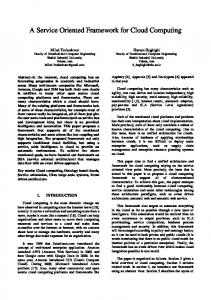
Vertical load-balancing across multiple implementation options

Enterprises may use a service-oriented architecture (SOA) to provide a streamlined interface to their business processes. To scale up the system, each tier in a composite service usually deploys multiple servers for load distribution and fault tolerance. Such load distribution across multiple servers within the same tier can be viewed as horizontal load distribution. One limitation of this approach is that load cannot be further distributed when all servers in the same tier are fully loaded. In complex multi-tiered systems, a single business process may actually be implemented by multiple different computation pathways among the tiers, each with different components, in order to provide resiliency and scalability. Such SOA-based enterprise computing with multiple implementation options gives opportunities for vertical load distribution across tiers. In this paper, we propose a requestrouting framework for SOA-based enterprise computing that takes into consideration both horizontal and vertical load distribution. Through experimentation we show that our algorithm and methodology scale well up to a large system configuration comprising up to 1000 workflow requests to a complex composite service with multiple implementations. We also show that a combination of both horizontal and vertical load distributions gives the maximum flexibility to improve performance and fault tolerance.

Implementation 1

Implementation 2

Web and Application Server (heavy preprocessing)

Web and Application Server (light preprocessing)

Database Server (light querying)

Database Server (heavy querying and processing via stored procedure execution)

Analytics Server (heavy processing) Horizontal load balancing across servers within a server pool

INTRODUCTION Figure 1: Horizontal and vertical load distribution.

A service-oriented architecture (SOA) can be used to provide a streamlined interface to underlying business processes. In enterprise computing, a published SOA may act as a programmatic front-end to an aggregation of building-block components distinguished as individual services and their

supporting servers (e.g. [5]). Incoming requests to this composite SOA must be routed to the correct components and their respective servers, and such routing must be scalable to support a large number of requests. These composite services can be represented as multiple tiers of component invocations. To scale up the system, each tier usually deploys multiple servers for load distribution and fault tolerance. Such load distribution across multiple servers within the same tier can be viewed as horizontal load distribution. One limitation of this approach is that load cannot be further distributed when all servers in a given tier are fully loaded as a result of misconfigured infrastructures — where too many servers are deployed at one tier while too few servers are deployed at another tier. In complex multi-tiered SOA systems, a single business process can actually be implemented by multiple different computation pathways through the tiers (where each path-

∗The author is currently affiliated with Microsoft and can be reached at [email protected]. †The author is currently affiliated with SAP Research Center, China, and can be reached at [email protected]. Permission to make digital or hard copies of portions of this work for personal or classroom use is granted without fee provided that copies Permission to copy without feefor all or part or of this material isadvantage granted provided are not made or distributed profit commercial and that copiesbear are not or and distributed direct commercial thatthe copies thismade notice the fullforcitation on the firstadvantage, page. the VLDB copyright notice and of the publication andthan its date appear, Copyright for components of the thistitle work owned by others VLDB and notice is must givenbethat copying is by permission of the Very Large Data Endowment honored. Base Endowment. To copy otherwise,Toorcopy to republish, on servers Abstracting with credit is permitted. otherwise,totopost republish, or redistribute to lists, a fee and/or permission from the totopost on servers or torequires redistribute to listsspecial requires prior specific publisher, ACM. permission and/or a fee. Request permission to republish from: VLDB ‘08, August 24-30, 2008, Inc. Auckland, Publications Dept., ACM, Fax New +1 Zealand (212) 869-0481 or Copyright 2008 VLDB Endowment, ACM 000-0-00000-000-0/00/00. [email protected]. PVLDB '08, August 23-28, 2008, Auckland, New Zealand Copyright 2008 VLDB Endowment, ACM 978-1-60558-305-1/08/08

996

way may have different components) in order to provide resiliency and scalability. Such SOA-based enterprise computing with multiple implementation options gives opportunities for vertical load distribution across tiers. While much research and industry work has focused on request provisioning by balancing load across the servers of one service [2, 8], there has been little work on balancing load across multiple implementations of a composite service, where each service can be implemented via pathways through different service types. The example in Figure 1 illustrates how we differentiate horizontal load distribution, where load can be spread across multiple servers for one service component, from vertical load distribution, where load can be spread across tiers by using multiple implementations of a given service. Here a composite online analytic task can be represented as a call to a Web and Application Server (WAS) to perform certain preprocessing, followed by a call from the WAS to a Database server (DB) to fetch required data set, after which the WAS forwards the data set to a dedicated Analytics Server (AS) for computationally-expensive data mining tasks. This composite task can have multiple implementations in a modern IT data center. An alternative implementation may invoke the database to perform data mining instead of having the dedicated analytics server perform this task. This alternative implementation provides vertical load distribution by allowing a job scheduler to select the WAS-andDB implementation when the analytics server is not available or heavily loaded. Multiple implementations are desirable for the purposes of fault tolerance, load-balancing, scalability, and flexibility, especially with regard to diverse runtime conditions and misconfigured infrastructures. Furthermore, this approach complements the reusability goals of SOA components; in our scheme each component plays an important role in enabling the feasibility and applicability of multiple implementations. In this paper we propose a framework for request-routing and load balancing, both horizontally and vertically, in SOAbased enterprise computing infrastructures. We suggest that a genetic search algorithm [10] is appropriate for exploring a very large solution space in order to properly route requests to implementations and assign service instances to servers. Through experimentation we show that our algorithm and methodology scale well up to a large system configuration comprising up to 1000 requests to a complex composite web service with multiple implementations. We also show that our approach that considers both horizontal and vertical load distribution is effective in dealing with a misconfigured infrastructure (i.e. where there are too many servers in one tier and too few servers in another tier). The key contributions of this paper are the following: • We identify the need for intelligent scheduling in workloads that consist of composite service requests. Our problem space lies in the relationship between requesters, implementation options, service types, and servers. • We discuss a framework for simultaneously handling both horizontal and vertical load distribution. • We provide a reference implementation of a search algorithm that is able to produce optimal (or nearoptimal) schedules based on a genetic search heuristic. The rest of this paper is organized as follows. In Section 2, we describe the system architecture and terminology used

997

in this paper. In Section 3, we describe how we model the problem and our algorithms for scheduling and distributing load for composite web services. In Section 4 we show experimental results, and in Section 5 we discuss related work. We conclude the paper in Section 6.

2. OVERVIEW In this section we give an overview of the system architecture and describe the terms used in this paper. In Figure 2 we show an example in which an analytic process runs on a Web and Application Server (WAS), a Database Server (DB), and a specialized Analytics Server (AS). The overall process can be implemented by one of three options (as shown in the upper-right of the figure): • Implementation 1: Executing some lightweight preprocessing at the WAS (more precisely, the WAS instance S1 ) and then having the DB complete most of the expensive analytic calculation (S2 ); or • Implementation 2: Fetching data from the DB (S4 ) to the WAS and then completing most of the expensive analytic calculation at the WAS (S3 ); or • Implementation 3: Executing some lightweight preprocessing at the WAS (S5 ), then having the DB fetch data (S6 ), and finally having the AS perform the remaining expensive analytic calculation (S7 ). There are three different service types required for the overall analytic process, namely the WAS service type, the DB service type, and the AS service type. S1 , S3 , and S5 are instances of the WAS service type since they are the services provided by the WAS. Similarly, S2 , S4 , and S6 are instances of the DB service type, and S7 is an instance of the AS service type. There are three kinds of servers: WAS servers (M1 , M2 , and M3 ); DB servers (M4 and M5 ); and AS servers (M6 ). Although a server can typically support any instance of its assigned service type, in general this is not always the case. Our example reflects this notion: each server is able to support all instances of its service type, except M2 and M4 are less powerful servers so that they cannot support computationally expensive service instances, S3 and S2 . Each server has a service level agreement (SLA) for each service instance it supports, and these SLAs are published and available for the scheduler. The SLA includes information such as a profile of the load versus response time and an upper bound on the request load size for which a server can provide a guarantee of its response time. The scheduler is responsible for routing and coordinating execution of composite services comprising one or more implementations. One of the scheduler’s outputs is the derived SLA resulting from the routing of the incoming requests to the implementations and eventually to the appropriate servers. Note that the scheduler can derive the SLA and the corresponding routing logic as well as handle the actual task of routing the requests. Alternatively, the scheduler can be used solely for the purpose of deriving SLA and routing logic while configuring content-aware routers, such as [3], for high performance and hardware-based routing. The scheduler can also be enhanced to perform the task of monitoring actual QoS achieved by workflow execution and by individual service providers. If the scheduler observes failure of certain service providers to their QoS published, it

SLA published by providers

Composite Service (CS)

Implementations for CS

SLA for S1, S3, S5 by M1 SLA for S1, S5 by M2 SLA for S1, S3, S5 by M3 SLA for S4, S6 by M4

Scheduler

SLA for S2, S4, S6 by M5 SLA for S7 by M6

Option 1

S1

S2

Option 2

S4

S3

Option 3

S5

S6

S7

SLA for CS by Scheduler Request Routing Logic

M3

M4

M6

S6

S7

S5 M1

M2

M3

M4

M5

S1

S1

S1

S4

S2

S3

S6

S4

S3

S5

S5

S6

S5

S7

Analytic Server service instances

DB service instances

WAS service instances

WAS service type provider

M6

DB service type provider

Analytic Server service type provider

Figure 2: Request routing for SOA-based enterprise computing with multiple implementation options. • Each implementation invokes several service types, such as a web application server, a DBMS, or a computational analytics server.

can recompute the feasible SLA and the routing logic in an on-demand manner to adapt to the runtime environment. In this paper, we focus on the problem of automatically deriving the routing logic of a composite service with consideration of both horizontal and vertical load distribution options. The scheduler is required to find an optimal combination of a set of variables illustrated in Figure 2 for a number of concurrent requests. Specifically, it must find the best assignment of a request to an implementation and within an implementation, the best assignment of service type instance to server. We discuss our scheduling approach next.

3.

• Each service type can be embodied by one of several instances of the service type, where each instance can have different computing requirements. For example, one implementation may require a heavy DBMS computation instance (such as through a stored procedure) and a light computational analytics instance, whereas another implementation may require light DBMS querying and heavy computational analytics. We assume that these implementations are set up by administrators or engineers.

SCHEDULING COMPOSITE SERVICES

• Each service type is executed on a server within a pool of servers dedicated to that service type.

In this section we formally define the problem and describe how we model its complexity. We provide a reference design for a heuristic to search the solution space and then discuss how we can extend this work to treat online arriving requests.

We assume that the servers make agreements to guarantee a level of performance defined by the completion time for completing a web service invocation. Although these SLAs can be complex, in this paper we assume for simplicity that the guarantees can take the form of a linear performance degradation under load, an approach similar to other published work on service SLAs (e.g. [5]). This guarantee is defined by several parameters: α is the expected completion time (for example, on the order of seconds) if the assigned workload of web service requests is less than or equal to β, the maximum concurrency, and if the workload is higher than β, the expected completion for a workload of size ω

3.1 Solution Space We assume the following scenario elements: • Requests for a workflow execution are submitted to a scheduling agent. • The workflow can be embodied by one of several implementations, so each request is assigned to one of these implementations by the scheduling agent.

998

Algorithm 1 Genetic Search Algorithm 1: FUNCTION Genetic algorithm 2: BEGIN 3: Time t 4: Population P (t) := new random Population 5: 6: while ! done do 7: recombine and/or mutate P(t) 8: evaluate(P (t)) 9: select the best P (t + 1) from P (t) 10: t := t + 1 11: end while 12: END

our case, a chromosome is a specific mapping of requeststo-implementations and instances-to-servers along with its associated workload execution time. Genetic algorithms are commonly used to find optimal exact solutions or nearoptimal approximations in combinatorial search problems such as the one we address. It is known that a GA provides a very good tradeoff between exploration of the solution space and exploitation of discovered maxima [9]. Note that the GA is not guaranteed to find the optimal solution since several of its steps are stochastic. Pseudocode for a genetic algorithm is shown in Algorithm 1. The GA executes as follows. The GA produces an initial random population of chromosomes. (Although research in the field has shown that the initial configuration does not have a significant impact [7], we reduced the effect of initial randomization by reading pre-generated initial chromosomes from disk.) The chromosomes then recombine, simulating sexual reproduction, to produce children using portions of both parents. Mutations in the children are produced with small probability to introduce traits that were not in either parent. The children with the best scores (in our case, the lowest workload execution times) are chosen for the next generation. The steps repeat for a fixed number of iterations (200 in our experiments), allowing the GA to converge toward the best chromosome. In the end it is hoped that the GA explores a large portion of the solution space. With each recombination, the most beneficial portion of a parent chromosome is ideally retained and passed from parent to child, so the best child in the last generation has the best mappings. To improve the GA’s convergence, we implemented elitism, where the best chromosome found so far is guaranteed to exist in each generation. We chose a GA for several reasons. From our own prior work, we are familiar with modeling problems with a GA and the factors that affect its performance and optimality convergence [14]. Additionally, the mappings used in our problem are ideally suited to array and matrix representations, allowing us to use prior GA research that aid in chromosome recombination [4]. Finally, we note that the GA takes a relatively long period of time to run: a typical configuration for 200 iterations ran on the order of one minute versus the few seconds of the competing algorithms described in Section 4. However, this duration is fairly arbitrary: since it is a progressive optimizer, more or less time can be spent depending on the desired degree of optimality. We believe that the time spent performing this optimization is outweighed by the improvements in workload running time.

is α + γ(ω − β) where γ is a fractional coefficient. In our experiments we vary α, β, and γ with different distributions. We would like to ideally perform optimal scheduling to simultaneously distribute the load both vertically (across different tiers by choosing different implementation options) and horizontally (across different servers supporting a particular service type). There are thus two stages of scheduling. In the first stage, the requests are assigned to the implementations. In the second stage each implementation has a known set of instances of a service type, and each instance is assigned to servers within the pool of servers for the instance’s service type. The solution space of possible scheduling assignments can be found by looking at the possible combinations of these assignments. Suppose there are R requests and M possible implementations. There are then M R possible assignments in the first stage. Suppose further there are on average T service type invocations per implementation, and each of these service types can be handled by one of S on average possible servers. Across all the implementations, there are then M · S T combinations of assignments in the second stage. It total, there are M R ·M ·S T = M (R+1) · S T total combinations. An exhaustive search through this solution space is prohibitively costly for all but the smallest configurations. In the next subsection we describe how we use a genetic search algorithm to look for the optimal scheduling assignments.

3.2 Genetic algorithm Given the solution space of M (R+1) · S T , the goal is to find the best assignments of requests to implementations and service type instances to servers in order to minimize the running time of the workload, thereby providing our desired vertical and horizontal balancing. To search through the solution space, we use a genetic algorithm (GA) global search heuristic that allows us to explore portions of the space in a guided manner that converges towards the optimal solutions [10] [9]. We note that a GA is only one of many possible approaches for a search heuristic; we use a GA only as one tool. Others heuristics are available, including A∗ , tabu search, simulated annealing, and steepest-ascent hill climbing. A GA is a good representative of a larger class of randomized search heuristics, and it further has the property that it can be run as a progressive optimizer where it can trade off running time with optimization precision. A GA is a computer simulation of Darwinian natural selection that iterates through various generations to converge toward the best solution in the problem space. A potential solution to the problem exists as a chromosome, and in

3.2.1 Chromosome representation of a solution We used two data structures in a chromosome to represent each of the two scheduling stages. In the first stage, R requests are assigned to M implementations, so its representative structure is simply an array of size R, where each element of the array is in the range of [0, M − 1]. The second stage where instances are assigned to servers is more complex. In Figure 3 we show an example chromosome that encodes one scheduling assignment. The representation is a 2-dimensional matrix that maps {implementation, service type instance} to a server. For an implementation i utilizing service type instance j, the (i, j)th entry in the table is the identifier for the server to which the request is assigned.

999

3.2.2 Chromosome recombination 1 2 3 4 5 6 7 8

1 2 3 4 5 6 7 8 9 10 +--------------------------------------| 2 6 9 7 8 11 10 12 14 13 | 3 6 7 8 9 11 11 14 14 13 | 1 5 8 7 8 11 10 13 13 13 | 0 5 8 9 8 10 10 13 14 13 | 3 6 7 7 9 10 11 14 14 13 | 4 5 7 7 9 10 11 13 14 12 | 4 5 9 9 7 11 11 13 13 14 | 0 5 8 9 8 11 11 12 12 13

Two parent chromosomes recombine to produce a new child chromosome. The hope is that the child contains the best contiguous chromosome regions from its parents. Recombining the chromosome from the first scheduling stage is simple since the chromosomes are simple 1-dimensional arrays. Two cut points are chosen randomly and applied to both the parents. The array elements between the cut points in the first parent are given to the child, and the array elements outside the cut points from the second parent are appended to the array elements in the child. This is known as a 2-point crossover. For the 2-dimensional matrix, chromosome recombination was implemented by performing a one-point crossover scheme twice (once along each dimension). The crossover is best explained by analogy to Cartesian space as follows. A random location is chosen in the matrix to be coordinate (0, 0). Matrix elements from quadrants II and IV from the first parent and elements from quadrants I and III from the second parent are used to create the new child. This approach follows GA best practices by keeping contiguous chromosome segments together as they are transmitted from parent to child, as shown in Figure 4. The uni-chromosome mutation scheme randomly changes one of the service provider assignments to another provider within the available range. Other recombination and mutation schemes are an area of research in the GA community, and we look to explore new operators in future work.

Figure 3:

An example chromosome representing a scheduling assignment of (implementation, service type instance) → server. Each row represents an implementation, and each column represents a service type instance. For example, here there are 8 workflows and 10 service types instances. In workflow 1, any request for service type 3 goes to server 9. Parent 1 0

1

2

3

4

0

1

2

0

2

1

1

0

1

0

1

0

2

1

2

0

0

1

3.2.3 GA evaluation function The evaluation function returns the resulting workload execution time given a chromosome. Note the function can be implemented to evaluate the workload in any way so long as it is consistently applied to all chromosomes across all generations. Our evaluation function is shown in Algorithm 2. In lines 6 to 8, it initializes the execution times for all the servers in the chromosome. In lines 11-17, it assigns requests to implementations and service type instances to servers using the two mappings in the chromosome. The end result of this phase is that the instances are accordingly enqueued at the servers. In lines 19-21 the running times of the servers are calculated. In lines 24-26, the results of the servers are used to compute the results of the implementations. The function returns the maximum execution time among the implementations.

Parent 2 0

1

2

3

4

0

0

0

0

1

1

1

1

2

0

0

0

2

1

1

0

2

1

Child 0

1

2

3

4

0

1

2

0

1

1

1

0

1

0

0

0

2

1

1

0

0

1

3.3 Handling online arriving requests As mentioned earlier, the problem domain we consider is that of batch-arrival request routing. We take full advantage of such a scenario through the use of the GA, which has knowledge of the request population. This approach can be further extended to online arriving requests using two techniques that we briefly describe next. We will explore and discuss this topic more thoroughly in future work. First, we can continue to use the GA, but instead of having the complete collection of requests available to us, we can allow requests to aggregate into a queue first. When a periodic timer expires, we can run the GA on those requests while aggregating any more incoming requests into another queue. Once the GA is finished with the first queue, it will process the next queue when the periodic timer expires again. If the request arrival rate is faster than the GA’s processing rate,

Figure 4: An example recombination between two parents to produce a child. Elements from quadrants II and IV from the first parent and elements from quadrants I and III from the second parent are used to create the new child.

1000

Experimental parameter Requests Implementations Service types used per implementation Instances per service type Servers per service type Server completion time (α) Server maximum concurrency (β) Server degradation coefficient (γ) GA: population size GA: number of generations

Comment 1 to 1000 5, 10, 20 uniform random: uniform random: uniform random: uniform random: uniform random: uniform random: 100 200

1 - 10 1 - 10 1 - 10 1 - 12 seconds 1 - 12 0.1 - 0.9

Table 1: Experimental parameters we can take advantage of the fact that the GA can be run as an incomplete, near-optimal search heuristic: we can go ahead and let the timer interrupt the GA, and the GA will have some solution that, although sub-optimal, is likely better than a greedy solution. This methodology is also shown in [6], where requests for broadcast messages are queued, and the messages are optimally distributed through the use of an evolutionary strategies algorithm (a close cousin of a genetic algorithm). Second (and unrelated to genetic algorithms), we can use online stochastic optimization techniques to serve online arrivals [19]. This approach approximates the offline problem by sampling historical arrival data in order to make the best online decision. An online optimizer receives an incoming sequence of requests, gets historical data over some period of time from a sampling function that creates a statistical distribution model, and then calculates and returns an optimized allocation of requests to available resources. This optimization can be done on a periodic or continuous basis.

Algorithm 2 GA evaluation function 1: FUNCTION evaluate 2: IN: CHROM OSOM E, a representation of the assignments of requests to implementation and service type instances to servers 3: OUT: runningtime, the running time of this workload 4: BEGIN 5: 6: for (each server ∈ CHROM OSOM E) do 7: set server’s running time to 0 8: end for 9: 10: {Loop over each request and its implementations} 11: for (each request ∈ CHROM OSOM E) do 12: implementation := requests’s implementation 13: for (each instance ∈ implementation) do 14: server := implementation’s server 15: Enqueue this job at server 16: end for 17: end for 18: 19: for (each server) do 20: Compute the running time of server 21: end for 22: 23: {Now compute implementations’ running times} 24: for (each implementation ∈ CHROM OSOM E) do 25: Aggregate the running time of this implementation across its instances 26: end for 27: 28: runningtime := maximum running time of each implementation 29: return runningtime 30: END

4. EXPERIMENTS AND RESULTS We ran experiments to show how our system compared to other well-known algorithms with respect to our goal of providing request routing with horizontal and vertical distribution. Since one of our intentions was to demonstrate how our system scales well up to 1000 requests and since there is no benchmark workload for SOA applications, we used a synthetic workload that allowed us to precisely control experimental parameters, including the number of available implementations, the number of published service types, the number of service type instances per implementation, and the number of servers per service type instance. The scheduling and execution of this workload was simulated using a program we implemented in standard C++. The simulation ran on an off-the-shelf Red Hat Linux desktop with a 3.0 GHz Pentium IV and 2GB of RAM. In these experiments we compared our algorithm against the following alternatives: • A round-robin algorithm that assigns requests to an implementation and service type instances to a server in circular fashion. This well-known approach provides a fast and simple scheme for load-balancing. • A random-proportional algorithm that proportionally assigns instances to the servers. For a given service type, the servers are ranked by their guaranteed completion time, and instances are assigned proportionally to the servers based on the servers’ completion time. (We also tried a proportionality scheme based on both

1001

Workload running time with 5 implementations

Workload running time with 10 implementations

700

600

Workload running time [seconds]

Workload running time [seconds]

600

700 Greedy Proportional Random Round-robin GA

500

400

300

200

100

Greedy Proportional Random Round-robin GA

500

400

300

200

100

0

0 100

200

300

400

500

600

700

800

900

1000

100

200

300

Number of requests

400

500

600

700

800

900

1000

Number of requests

Figure 5: Response time with 5 implementations.

Figure 6: Response time with 10 implementations. Workload running time with 20 implementations

the completion times and maximum concurrency but attained the same results, so only the former scheme’s results are shown here.) To isolate the behavior of this proportionality scheme in the second phase of the scheduling, we always assigned the requests to the implementations in the first phase using a round-robin scheme.

700

Workload running time [seconds]

600

• A purely random algorithm that randomly assigns requests to an implementation and service type instances to a server in random fashion. Each choice was made with a uniform random distribution. • A greedy algorithm that always assigns business processes to the service provider that has the fastest guaranteed completion time. This algorithm represents a naive approach based on greedy, local observations of each workflow without taking into consideration all workflows.

Greedy Proportional Random Round-robin GA

500

400

300

200

100

0 100

200

300

400 500 600 Number of requests

700

800

900

1000

Figure 7: Response time with 20 implementations.

In the future we will look to implement more algorithms for comparison, such as first-fit. Scheduling and assignment algorithms are a research topic unto themselves, and there is a very wide of range of approaches that may be explored. In the experiments that follow, all results were averaged across 20 trials, and to help normalize the effects of any randomization, each trial started by reading in pre-initialized data from disk. In Table 1 we list our experimental parameters for our baseline experiments. We vary these parameters in other experiments, as we discuss later.

servers than the other algorithms. The GA shows a 45% improvement over its nearest competitor (typically the roundrobin algorithm) with a configuration of 5 implementations and 1000 requests and a 36% improvement in the largest configuration with 20 implementations and 1000 requests. The relative behavior of the other algorithms was consistent. The greedy algorithm performed the worst while the random-proportional and random algorithms were close together. The round-robin came the closest to the GA. To better understand these results, we looked at the individual behavior of the servers after the instance requests were assigned to them. In Figure 8 we show the percentage of servers that were saturated among the servers that were actually assigned instance requests. These results were from the same 10-implementation experiment from Figure 6. For clarity, we focus on a region with up to 300 requests. We consider a server to be saturated if it was given more requests than its maximum concurrency parameter. From this graph we see the key behavior that the GA is able to find assignments well enough to delay the onset of saturation until 300 requests. The greedy algorithm, as can be expected, always targets the best server from the pool available for a given service type and quickly causes these chosen servers to saturate. The round robin is known to be a quick and easy way to spread load and indeed provides the lowest satura-

4.1 Baseline configuration results In Figures 5, 6, and 7 we show the behavior of the algorithms as they schedule requests against 5, 10, and 20 implementations, respectively. In each graph, the x-axis shows the number of requests (up to 1000), and the y-axis is average response time upon completing the workload. This response time is the makespan, the metric commonly used in the scheduling community and calculated as the maximum completion time across all requests in the workload. As the total number of implementations increases across the three graphs, the total number of service types, instances, and servers scaled as well in accordance to the distributions of these variables from Table 1. In each of the figures, it can be see that the GA is able to produce a better assignment of requests to implementations and service type instances to

1002

tion up through 60 requests. The random-proportional and random algorithms reach saturation points between that of the greedy and GA algorithms.

Servers saturated

1

4.2 Effect of service types We then varied the number of service types per implementation, modeling a scenario where there is a heavily skewed number of different web services available to each of the alternative implementations. Intuitively, in a deployment where there is a large number of services types to be invoked, the running time of the overall workload will increase. In Figure 9 we show the results where we chose the numbers of service types per implementation from a Gaussian distribution with a mean of 2.0 service types; this distribution is in contrast to the previous experiments where the number was selected from a uniform distribution in the inclusive range of 1 to 10. As can be seen, the algorithms show the same relative performance from prior results in that the GA is able to find the scheduling assignments resulting in the lowest response times. The worst performer in this case is the random algorithm. In Figure 10 we skew the number of service types in the other direction with a Gaussian distribution with a mean of 8.0. In this case the overall response time increases for all algorithms, as can be expected. The GA still provides the best response time.

Percentage of servers

0.8

0.6

0.4

0.2

Greedy Proportional Random Round-robin GA

0 50

100

150 Number of requests

200

250

300

Figure 8: Percentage of servers that were saturated. A saturated server is one whose workload is greater than its maximum concurrency.

Workload running time with skewed distribution of service types per implementation 700

600

Workload running time [seconds]

4.3 Effect of service type instances In these experiments we varied the number of instances per service type. We implemented a scheme where each instance incurs a different running time on each server; that is, a unique combination of instance and server provides a different response time, which we put into effect by a Gaussian random number generator. This approach models our target scenario where a given implementation may run an instances that performs more or less of the work associated with the instance’s service type. For example, although two implementations may require the use of a DBMS, one implementation’s instance of this DBMS task may require less computation than the other implementation due to the offload of a stored procedure in the DBMS to a separate analytics server. Our expectation is that having more instances per service type allows a greater variability in performance per service type. Figure 11 shows the algorithm results when we skewed the number of instances per service type with a Gaussian distribution with a mean of 2.0 instances. Again, the relative ordering shows that the GA is able to provide the lowest workload response among the algorithms throughout. When we weight the number of instances with a mean of 8.0 instances per service type, as shown in Figure 12, we can see that the the GA again provides the lowest response time results. In this larger configuration, the separation between all the algorithms is more evident with the greedy algorithm typically performing the worst; its behavior is again due the fact that it assigns jobs only to the best server among the pool of servers for a service type.

Greedy Proportional Random Round-robin GA

500

400

300

200

100

0 100

200

300

400

500

600

700

800

900

1000

Number of requests

Figure 9: Average response time with a skewed distribution of service types per implementation. The distribution was Gaussian (λ = 2.0, σ = 2.0 service types).

Workload running time with skewed distribution of service types per implementation 700

Workload running time [seconds]

600

Greedy Proportional Random Round-robin GA

500

400

300

200

100

4.4 Effect of servers (horizontal balancing)

0 100

Here we explored the impact of having more servers available in the pool of servers for the service types. This experiment isolates the effect of horizontal balancing. Increasing the size of this pool will allow assigned requests to be spread out and thus reduce the number of requests per server, re-

200

300

400 500 600 Number of requests

700

800

900

1000

Figure 10: Average response time with a skewed distribution of service types per implementation. The distribution was Gaussian (λ = 8.0, σ = 2.0 service types).

1003

Workload running time with skewed distribution of instances per service type 700

600

Greedy Proportional Random Round-robin GA

Workload running time with skewed distribution of servers per service type 700

500 Workload running time [seconds]

Workload running time [seconds]

600

Greedy Proportional Random Round-robin GA

400

300

200

500

400

300

200

100 100 0 100

200

300

400

500

600

700

800

900

1000 0

Number of requests

100

200

300

Figure 11: Average response time with a skewed distribution of instances per service type. The distribution was Gaussian (λ = 2.0, σ = 2.0 instances).

400 500 600 Number of requests

700

800

900

1000

Figure 13: Average response time with a skewed distribution of servers per service type. The distribution was Gaussian (λ = 2.0, σ = 2.0 instances).

Workload running time with skewed distribution of instances per service type 700

600

Greedy Proportional Random Round-robin GA

Workload running time with skewed distribution of servers per service type

500 600

Greedy Proportional Random Round-robin GA

400 Workload running time [seconds]

Workload running time [seconds]

700

300

200

100

500

400

300

200

0 100

200

300

400 500 600 Number of requests

700

800

900

1000

100

Figure 12: Average response time with a skewed dis-

0 100

tribution of instances per service type. The distribution was Gaussian (λ = 8.0, σ = 2.0 instances).

200

300

400 500 600 Number of requests

700

800

900

1000

Figure 14: Average response time with a skewed distribution of servers per service type. The distribution was Gaussian (λ = 8.0, σ = 2.0 instances).

sulting in lower response times for the workload. In Figures 13 and 14 we show the results with Gaussian distributions with means of 2.0 and 8.0, respectively. In both graphs the GA appears to provide the lowest response times. Furthermore, it is interesting to note that in the random, randomproportional, and round-robin algorithms, the results did not change substantially between the two experiments even though the latter experiment contains four times the average number of servers. We believe this result may be due to the fact that the first-stage scheduling of requests to implementations is not taking sufficient advantage of the second-stage scheduling of service type instances to the increased number of servers. Since the GA is able to better explore all combinations across both scheduling stages, it is able to produce its better results. We will explore this aspect in more detail in the future.

Workload running time with skewed distribution of servers’ completion time 700

Workload running time [seconds]

600

Greedy Proportional Random Round-robin GA

500

400

300

200

100

4.5 Effect of server performance

0 100

In this subsection we look at the impact on the servers’ individual performance on the overall workload running time. In previous sections we described how we modeled each server with variables for the response time (α) and the concurrency (β). Here we skewed these variables to show how

200

300

400

500

600

700

800

900

1000

Number of requests

Figure 15: Average response time with a skewed distribution of servers’ completion time. The distribution was Gaussian (λ = 2.0, σ = 2.0 seconds).

1004

the algorithms performed as a result. In Figures 15 and 16 we skewed the completion times with Gaussian distributions with means of 2.0 and 9.0, respectively. It can be seen that the relative orderings of the algorithms are roughly the same in each, with the GA providing best performance, the greedy algorithm giving the worst, and the other algorithms running in between. Surprisingly, the difference in response time between the two experiments was much less than we expected, although there is a slight increase in all the algorithms except for the GA. We believe that the lack of a dramatic rise in overall response time is due to whatever load balancing is being performed by the algorithms (except the greedy algorithm). We then varied the maximum concurrency variable for the servers using Gaussian distributions with means of 4.0 and 11.0, as shown in Figures 17 and 18. From these results it can be observed that the algorithms react well with an increasing degree of maximum concurrency. As more requests are being assigned to the servers, the servers respond with faster response times when they are given more headroom to run with these higher concurrency limits.

Workload running time with skewed distribution of servers’ completion time 700

Workload running time [seconds]

600

Greedy Proportional Random Round-robin GA

500

400

300

200

100

0 100

200

300

400 500 600 Number of requests

700

800

900

1000

Figure 16: Average response time with a skewed distribution of servers’ completion time. The distribution was Gaussian (λ = 9.0, σ = 2.0 seconds).

4.6 Effect of response variation control

Workload running time with skewed distribution of servers’ maximum concurrency

We additionally evaluated the effect of having the GA minimize the variation in the requests’ completion time. As mentioned earlier, we have been been calculating the workload completion as the maximum completion time of the requests in that workload. While this approach has been effective, it produces wide variation between the requests’ completion times due to the stochastic packing of requests by the GA. This variation in response time, known as jitter in the computer networking community, may not be desirable, so we further provided an alternative objective function that minimizes the jitter (rather than minimizing the workload completion time). In Figure 19 we show the average standard deviations resulting from these different objective functions (using the same parameters as in Figure 6). With variation minimization on, the average standard deviation is always close to 0, and with variation minimization off, we observe an increasing degree of variation. The results in Figure 20 show that the reduced variation comes at the cost of longer response times.

700

Workload running time [seconds]

600

Greedy Proportional Random Round-robin GA

500

400

300

200

100

0 100

200

300

400 500 600 Number of requests

700

800

900

1000

Figure 17: Average response time with a skewed distribution of servers’ maximum concurrency. The distribution was Gaussian (λ = 4.0, σ = 2.0 jobs).

4.7 Effect of routing against conservative SLA Workload running time with skewed distribution of servers’ maximum concurrency

We looked at the GA behavior when its input parameters were not the servers’ actual parameters but rather the parameters provided by a conservative SLA. In some systems, SLAs may be defined with a safety margin in mind so that clients of the service do not approach the actual physical limits of the underlying service. In that vein, we ran an experiment similar to that shown in Figure 6, but in this configuration we used parameters for the underlying servers with twice the expected response time and half the available parallelism, mirroring a possible conservative SLA. As can be seen in Figure 21, the GA converges towards a scheduling where the extra slack given by the conservative SLA results in a slower response time.

700

Workload running time [seconds]

600

Greedy Proportional Random Round-robin GA

500

400

300

200

100

0 100

200

300

400

500

600

700

800

900

4.8 Summary of experiments

1000

Number of requests

In this section we evaluated our GA reference implementation of a scheduler that performs request-routing for horizontal and vertical load distribution. We showed that the GA consistently produces lower workload response time than its

Figure 18: Average response time with a skewed distribution of servers’ maximum concurrency. The distribution was Gaussian (λ = 11.0, σ = 2.0 jobs).

1005

competitors. Furthermore, as can be expected, the scheduler is sensitive to a number of parameters, including the number of service types in each implementation, the number of service type instances, the number of servers, the per-server performance, the desired degree of variation, and the tightness of the SLA parameters.

Request response time standard deviation, with/without variation minimization 25

Standard deviation of request response time

GA, variation minimization on GA, variation minimization off

20

5. RELATED WORK

15

[16] described a distributed quality of service (QoS) management architecture and middleware that accommodates and manages different dimensions and measures of QoS. The middleware supports the specification, maintenance, and adaptation of end-to-end QoS (including temporal requirements) provided by the individual components in complex real time application systems. Using QoS negotiation, the middleware determines the quality levels and resource allocations of the application components. This work focused on analysis tradeoff between QoS and cost instead of ensuring QoS requirements in our paper. [20] presented two algorithms for finding replacement services in autonomic distributed business processes when web service providers fail to meet the QoS requirement: (i) follow alternative predefined routes or (ii) find alternative routes on demand. This approaches provide the QoS brokerage service with a fault tolerance capability and are complementary to our work. [21, 22, 23] discuss a set of algorithms for Web services selection with end-to-end QoS constraints. A key point is that these algorithms simplify and reduce the complexity space considerably, something which we do not do. These methods take all incoming workflows, aggregate them into one single workflow, and then schedule the one workflow onto the underlying service providers. We do not do this aggregation, and therefore our approach provides a higher degree of scheduling flexibility. In the work [14], a genetic algorithm was used for load distribution of analytic workloads across a database cluster. The load distribution algorithm found near-optimal placements for the collocation of queries and their needed MQTs (i.e. materialized views), the collocation of MQTs and the base tables required to construct the MQTs, and the minimization of the execution time of the whole workload on the database cluster. This work may be considered a type of horizontal load distribution. Additionally, a genetic algorithm is also used in [13] to find a near-optimal view materialization permutation for minimal overall execution time of workloads. Our work is related to prior efforts in web service composition, web service scheduling, and job scheduling. A web service’s interface is expressed in WSDL, and given a set of web services, a workflow can be specified in a flow language such as BPEL4WS [11] or WSCI [12]. Several research projects have looked to provide automated web services composition using high-level rules (e.g. eFlow [1], SWORD [15]). Our work is complementary to this area, as we schedule business processes within multiple, already-defined workflows to the underlying servers. In the context of service assignment and scheduling, [24] maps web service calls to potential servers, but their work is concerned with mapping only single workflows; our principal focus is on scalably scheduling multiple workflows (up to one thousand). [18] presents a dynamic provisioning approach that uses predictive and reactive techniques for

10

5

0 100

200

300

400

500

600

700

800

900

1000

Number of requests

Figure 19: Average standard deviation from the mean response for two different objective functions.

Workload running time of GA with/without variation minimization 700 GA, variation minimization on GA, variation minimization off

Workload running time [seconds]

600

500

400

300

200

100

0 100

200

300

400 500 600 Number of requests

700

800

900

1000

Figure 20: Average response time for two different objective functions.

Workload running time with 10 implementations, with and without conservative SLA-based routing 700 Conservative SLA Normal SLA

Workload running time [seconds]

600

500

400

300

200

100

0 100

200

300

400

500

600

700

800

900

1000

Number of requests

Figure 21: Response time with 10 implementations for normal and conservative SLA.

1006

multi-tiered Internet application delivery. However, the provisioning techniques do not consider the challenges faced when there are alternative execution paths and replicated data sources. [17] presents a feedback-based scheduler for multi-tiered systems with back-end databases, but unlike our work, it assumes a tighter coupling between the various components of the system.

6.

[9] D. Goldberg. Genetic Algorithms in Searth, Optimization, and Machine Learning. Kluwer Academic, 1989. [10] J. Holland. Adaptation in Natural and Artificial Systems. MIT Press, 1992. [11] IBM. Business process execution language for web services, v 1.1, 2005. www-128.ibm.com/developerworks/library/ws-bpel/. [12] J. Josephraj. Web Services Choreography in Practice. In www-128.ibm.com/developerworks/library/wschoreography. [13] T. Phan and W.-S. Li. Dynamic Materialization of Query Views for Data Warehouse Workloads. In ICDE, 2008. [14] T. Phan and W.-S. Li. Load Distribution of Analytical Query Workloads for Database Cluster Architectures. In EDBT, 2008. [15] S. Ponnekanti and A. Fox. Interoperability among Independently Evolving Web Services. In Proceedings of Middleware, 2004. [16] M. Shankar, M. De Miguel, and J. W.-S. Liu. An end-to-end qos management architecture. In Proceedings of the Fifth IEEE Real Time Technology and Applications Symposium. [17] G. Soundararajan, K. Manassiev, J. Chen, A. Goel, and C. Amza. Back-end Databases in Shared Dynamic Content Server Clusters. In ICAC, 2005. [18] B. Urgaonkar, P. Shenoy, A. Chandra, and P. Goyal. Dynamic Provisioning of Multi-Tier Internet Applications. In Proceedings of ICAC, 2005. [19] P. Van Hentenryck and R. Bent. Online Stochastic Combinatorial Optimization. MIT Press, 2006. [20] T. Yu and K.-J. Lin. Adaptive algorithms for finding replacement services in autonomic distributed business processes. In Proc. of the 7th International Symposium on Autonomous Decentralized Systems, Chengdu, China, 2005. [21] T. Yu and K.-J. Lin. Service selection algorithms for web services with end-to-end qos constraints. Inf. Syst. E-Business Management, 3(2):103–126, 2005. [22] T. Yu and K.-J. Lin. Qcws: An implementation of qos-capable multimedia web services. Multimedia Tools and Applications, 30(2):165–187, 2006. [23] T. Yu, Y. Zhang, and K.-J. Lin. Efficient algorithms for web services selection with end-to-end qos constraints. ACM Transactions on the Web (TWEB), 1(1), 2007. [24] L. Zeng, B. Benatallah, M. Dumas, J. Kalagnanam, and Q. Sheng. Quality Driven Web Services Composition. In Proceedings of WWW, 2003.

CONCLUSION AND FUTURE WORK

Enterprises may use an SOA to provide a streamlined interface to their business processes. To scale up the number of business processes, each tier usually deploys multiple servers for load distribution and fault tolerance. Such load distribution across multiple servers within the same tier can be viewed as horizontal load distribution. One limitation of this approach is that load cannot be further distributed when all servers in the same tier are fully loaded. Another option for providing resiliency and scalability is to support multiple implementation options that give opportunities for vertical load distribution across tiers. In this paper, we propose a request-routing framework for SOA-based enterprise computing that takes into consideration both horizontal and vertical load distribution. Specifically, a job scheduler finds the best assignment of a request to an implementation and a service type instance to a server. Experiments show that our algorithm and methodology can scale well up to a large scale system configuration comprising up to 1000 workflow requests to a complex composite service with multiple implementation options available. The results also show that our framework is more agile in the sense it is effective in dealing with misconfigured infrastructures in which there are too many or too few servers in one tier. We look to extend our work in a number of directions. We hope to obtain a real-world SOA trace to complement our synthetic workload. Additionally, we will compare other search heuristics to the GA, including other randomized heuristics as well as greedy approximation algorithms. Finally, in a later journal version of this paper, we will explore our experimental results in finer detail, particularly the impact of having more servers for horizontal balancing.

7.

REFERENCES

[1] F. Casati, S. Ilnicki, L. Jin, V. Krishnamoorthy, and M.-C. Shan. Adaptive and Dynamic Service Composition in eFlow. In Proceedings of CAISE, 2000. [2] Cisco. Ace application-level load balancer. [3] Cisco. Scalable content switch. [4] L. Davis. Job Shop Scheduling with Genetic Algorithms,. In Proceedings of the International Conference on Genetic Algorithms, 1985. [5] G. DeCandia, D. Hastorun, M. Jampani, G. Kakulapati, A. Lakshman, A. Pilchin, S Sivasubramanian, P. Vosshall, and W. Vogels. Dynamo: Amazon’s highly available key-value store. In SOSP, 2007. [6] R. Dewri, I. Ray, I. Ray, and D. Whitley. Optimizing on-demand data broadcast scheduling in pervasive environments. In EDBT, 2008. [7] A. E. Eiben and J. E. Smith. Introduction to Evolutionary Computing. Springer, 1998. [8] F5 Networks. Big-ip application-level load balancer.

1007