A Review of Bayesian Variable Selection Methods - CiteSeerX

Bayesian Analysis (2009)

4, Number 1, pp. 85–118

A Review of Bayesian Variable Selection Methods: What, How and Which R.B. O’Hara∗ and M. J. Sillanp¨a¨a† Abstract. The selection of variables in regression problems has occupied the minds of many statisticians. Several Bayesian variable selection methods have been developed, and we concentrate on the following methods: Kuo & Mallick, Gibbs Variable Selection (GVS), Stochastic Search Variable Selection (SSVS), adaptive shrinkage with Jeffreys’ prior or a Laplacian prior, and reversible jump MCMC. We review these methods, in the context of their different properties. We then implement the methods in BUGS, using both real and simulated data as examples, and investigate how the different methods perform in practice. Our results suggest that SSVS, reversible jump MCMC and adaptive shrinkage methods can all work well, but the choice of which method is better will depend on the priors that are used, and also on how they are implemented. Keywords: Variable Selection, MCMC, BUGS

1

Introduction

An important problem in statistical analysis is the choice of an optimal model from a set of a priori plausible models. In many analyses, this reduces to the choice of which subset of variables should be included into the model. This problem has exercised the minds of many statisticians, leading to a variety of algorithms for searching the model space and selection criteria for choosing between competing models (e.g. Miller 2002; Broman and Speed 2002; Sillanp¨a¨a and Corander 2002). In the Bayesian framework, the model selection problem is transformed to the form of parameter estimation: rather than searching for the single optimal model, a Bayesian will attempt to estimate the posterior probability of all models within the considered class of models (or in practice, of all models with non-negligible probability). In many cases, this question is asked in variable-specific form: i.e. the task is to estimate the marginal posterior probability that a variable should be in the model. At present, the computational method most commonly used for fitting Bayesian models is Markov chain Monte Carlo (MCMC) technique (Robert and Casella 2004). Variable selection methods are therefore needed that can be implemented easily in the MCMC framework. In particular, having these models implemented in the BUGS language (either in WinBUGS or OpenBUGS) means that the methods can easily be slotted into different models. The purpose of this paper is to review the different methods that ∗ Department

of Mathematics and Statistics, University of Helsinki, Finland, mailto:bob.ohara@ helsinki.fi ∗ Department of Mathematics and Statistics, University of Helsink i, Finland, http://www.rni. helsinki.fi/~mjs/

c 2009 International Society for Bayesian Analysis °

DOI:10.1214/09-BA403

86

Bayesian Variable Selection Methods

have been suggested for variable selection, and to present BUGS code for their implementation, which may also help to clarify the ideas presented. Some of these methods have been reviewed by Dellaportas et al. (2000). We do not consider some methods, such as Bayesian approximative computational approaches (e.g. Ball 2001; Sen and Churchill 2001) or methods based on calculating model choice criteria, such as DIC (Spiegelhalter et al. 2002), because these are only feasible to use with a maximum of dozens of candidate models. We also omit the machine learning literature focusing on finding maximum a posteriori estimates for parameters (e.g. Tipping 2004). Although methods for variable selection are reviewed here, this should not be taken to imply that they should be used uncritically. In many studies, the variables in the regression have been chosen because there is a clear expectation that they will influence the response, and the problem is one of inferring the strength of influence. For these studies, the best strategy may therefore be to fit the full model, and then interpret the sizes of the posterior estimates of the parameters in terms of their importance. In other studies the purpose is more exploratory: seeing what the analysis throws out from a large number of candidates. This is not always an unreasonable approach. One clear example where this is a sensible way to proceed is in gene mapping, where it is assumed that there are only a small number of genes that have a large effect on a trait, while most of the genes have little or no effect. The underlying biology is therefore sparse: only a few factors (i.e. genes) are expected to influence the trait. The distinction between this case, and many other regression problems is in the prior distribution of effect sizes: for gene mapping, the distribution is extremely leptokurtic, with a few large effects, but most regression coefficients being effectively zero. The prior is also exchangeable over the loci (i.e. we are ignorant a priori of where any influential gene might be located). Conversely, in many studies the expectation may be of a slow tapering of effects, with no clear tail to the distribution, and often more substantial information about the likely size of the effects. This implies that a different set of priors should be considered in these two situations: this paper examines different options for the exploratory case where the prior may be leptokurtic. This review is structured so that we first set out the general regression model. We then describe the different variable selection methods, and some of their properties. Then we describe three examples, using simulated and real data sets, to illustrate the performance of the different methods. Finally, we wrap up by discussing the relative merits of these methods, and indicate when different methods might be preferred. BUGS code for the methods is given in Supplementary Material online, as are some supplementary figures.

R.B. O’Hara and M. J. Sillanp¨a¨a

2 2.1

87

The Bayesian Variable Selection Methods Description of sparse selection problem

The problem is the familiar regression problem of trying to explain a response variable with a (large) number of explanatory variables (whether continuous or discrete factors). The aim is to select a small subset of the variables whilst controlling the rate of false detection, so that it can be inferred that these variables explain the a large fraction of the variation in the response. We may have some a priori knowledge or expectation that only a small proportion of candidates are truly affecting the outcome, and ideally this information should be taken into account in the variable selection. The optimal degree of sparseness and how many false detections are allowed is very problem-specific. One aspect of the problem is the well known trade-off between bias and variance. In general, a large set of variables is desirable for prediction and a small set of variables (that have a meaningful interpretation) for inference. Another aspect that influences the number of variables in the model is the number of observations in the data set. As a rule of thumb for shrinkage methods, one can safely consider only problems where there are maximally 10-15 times more candidates than observations (Zhang and Xu 2005; Hoti and Sillanp¨a¨a 2006). However, where the true and safe upper limit exists, is very problem specific and depends on degree of correlation (co-linearity) among the candidate variables.

2.2

Regression model

To keep the presentation simple, assume that the task is to explain an outcome yi for individual i (i = 1, ..., N ) using p covariates with values xi,j , j = 1, .., p. Naturally, these may be continuous or discrete (dummy) variables. Given a vector of regression parameters θ = (θj ) of size p, the response yi is modeled as a linear combination of the explanatory variables xi,j : yi = α +

p X

θj xi,j + ei .

(1)

j=1

Here, α is the intercept and ei ∼ N (0, σ 2 ) are the errors. We can assume more generally that yi is a member of the exponential family of distributions, giving us a generalized linear model. In such a case, we take the usual link function g(·) so that E(g(yi )) = ηi and ηi equals the right hand side of the linear model (1) without the error term. The variable selection procedure can be seen as one of deciding which of the regression parameters, the θj s, are equal to zero. Each θj should therefore have a “slab and spike” prior (Miller 2002), with a spike (the probability mass) either exactly at or around zero, and a flat slab elsewhere. For this, we may use an auxiliary indicator variable Ij (where Ij = 1 indicates presence, and Ij = 0 absence of covariate j

88

Bayesian Variable Selection Methods

in the model) to denote whether the variable is in the slab or spike part of the prior. A second auxiliary variable, the effect size βj , is also needed for most of the methods, where βj = θj when Ij = 1 (e.g. by defining θj = Ij βj ). When Ij = 0, the variable βj can be defined in several ways, and this leads to the differences between the methods outlined below. For the moment we will assume θj = Ij βj , to simplify the explanation, and change it later on when needed (e.g. for SSVS below). Once the model has been set up, it is usually fitted using MCMC, and many of the methods outlined below use a single-site Gibbs sampler to do this. The variable selection part of the model entails estimating Ij and θj . From this, the posterior probability that a variable is “in” the model, i.e. the posterior inclusion probability, can simply be calculated as the mean value of the indicator Ij . The methods outlined below vary in how they treat Ij , βj and θj .

2.3

Concepts and Properties

The methodologies of Bayesian variable selection and the differences between them can be best understood using several properties and concepts, which are described here. Sparseness The degree of sparseness required, i.e. how complex the model should be is an important property. In some cases, the sparseness may be set according to some optimality criterion (e.g. the best predictive abilities, (Burnham and Anderson 2002)). Taking a decision analytic perspective, we can view the prior as providing a loss function, so unless an objective optimality criterion can be found, it is not clear that one loss function is appropriate for all circumstances. Therefore, some flexibility in the amount of model complexity allowable is needed. An obvious approach to this is to use P (Ij = 1), the prior probability of variable inclusion, to set the sparseness: a smaller value of P (Ij = 1) leading to sparser models. Typically, this will be independent across the js, so that the prior distribution for the number of covariates is binomial, with mean P (Ij = 1). A value of 0.5 for this has been suggested for P (Ij = 1) (e.g. George and McCulloch 1993), which makes all models equiprobable. Whilst this may improve mixing properties of the MCMC sampler and may appear attractive as a null prior, it is informative in that it favours models where about half of the variables are selected. In many cases, only a small proportion of variables are likely to be required in the model, so this prior may often bias the model towards being too complex. The choice of value for P (Ij = 1) is then up to the investigator, in some cases a decision analytic approach may be a good way of eliciting the prior.

R.B. O’Hara and M. J. Sillanp¨a¨a

89

Tuning A practical problem in implementing variable selection is tuning the model (by adjusting different components, such as the prior distribution) to ensure good mixing of the MCMC chains, i.e. letting the sampler jump efficiently between the slab and spike. If single-site updaters are being used, this means updating Ij given a value of βj . This relies on confounding of Ij and βj , so that θj ≈ 0 for both Ij = 1 and Ij = 0, and hence the updater for Ij can jump between states easily (and θj be updated subsequently). In general, this will depend on the prior for θj , so the mixing properties of the sampler depend on the prior distributions. This has lead to the suggestion that data-based priors should be designed with the purpose of improving mixing (see references below) or giving good centering and scaling properties (e.g. a fractional prior, Smith and Kohn 2002). Although this is attractive from the computational point of view, it contravenes the Bayesian philosophy, as the prior should be a summary of the beliefs of the analyst (before seing the data), not a reflection of the ability of the fitting algorithms to do their job. One goal of this review is to find out under what circumstances the different methods work efficiently, so that philosophically correct (subjective) priors can be designed properly. This may require a trade-off, with a sub-optimal model being used, in order to accommodate better (philosophically plausible) priors. Several of the methods below may exhibit problems in the marginal identifiability (i.e. confounding) of variables Ij and βj . This can occur because almost identical likelihoods can be obtained for Ij = 1 and Ij = 0 when βj is near zero, as illustrated above. Deliberate confounding of variables can thus be used as a strategy to improve mixing. Because of this, though, it may be more informative to monitor the posterior of the product θj = Ij × βj instead of the individual variables (Sillanp¨a¨a and Bhattacharjee 2005), i.e. monitor the parameter that appears in equation 1.

Global adaptation A natural Bayesian strategy for building a model would be to place a normal prior on βj | (Ij = 1). If the variance of this prior is fixed at a constant, the model for the data would be equivalent to a classical fixed effects model, a terminology we will adopt here. But variable selection approaches can be developed where the variance is estimated as well. In some circumstances, this can be done by extending the model (1) above as a hierarchical model; considering the regression coefficients to be exchangeable and be drawn from a common distribution, e.g. βj | (Ij = 1) is drawn from N (0, τ 2 ), where τ 2 is an unknown parameter to be estimated. We will follow the terminology in classical statistics and refer to this as a random effect model. This approach has the advantage of helping tuning, for example if we define θj = βj Ij , then βj | (Ij = 0) will also depend on τ 2 . The distribution of θj is thus shrunk towards the correct region of the parameter space by the other θj s. This can help circumvent tuning problems, at the cost of increasing the confounding of Ij and βj , as is discussed more below.

90

Bayesian Variable Selection Methods

Local adaptation Instead of fitting one common parameter for all the regression coefficients, as in global adaptation, one can use different variance parameters for different covariates (or for covariate groups). This helps tuning and allows heterogeneity, i.e., if there are some local characteristics among covariates. An example of this is where βj | (Ij = 1) is drawn from N (0, τj2 ), where τj2 is an covariate-specific variance parameter to be estimated (cf. Example 2 in (Iswaran and Rao 2005)).

Analytical integration To speed up the convergence of the MCMC (and mixing with respect to selected covariates) in some of the model selection methods described above, it is possible to analytically integrate over the effects θ and σ 2 in model (1), and then use Gibbs sampling for the indicator variables (George and McCulloch 1997). Fast mixing is possible because updating an indicator does not depend on values of the effect coefficients. If preferred, the posterior for effect coefficients can still be obtained. Additionally in high dimensional problems, the coefficients βj only need to be updated for covariates with Ij = 1 (e.g. Yi 2004).

Bayesian Model Averaging One characteristic of the Bayesian approach is the ability to marginalize over nuisance parameters. This carries over into model selection, where posterior distributions of parameters (including indicators for models) can be calculated by averaging over all of the other variables, i.e. over the different models. For example, as we will do below, the probability that a single variable should enter a model can be averaged over all of the models. Of course, this is convenient in the MCMC framework as it just means that the calculations can be done on the MCMC output for each indicator (i.e. Ij ) separately. It is also well known that, with many covariates, it is the ones that have a large effect that are selected, even if support for estimated effect size is large by chance (e.g. Miller 2002; Lande and Thompson 1990; G¨oring et al. 2001). Hence, if the same data is used for estimating both the the model (i.e. variable selection) and individual contributions (effect sizes), overestimation of effect sizes will almost certainly occur. Fortunately, robust estimation of effect sizes can be done in a Bayesian setting by averaging the effect size over several different models (e.g. Ball 2001; Sillanp¨a¨a and Corander 2002). Given posterior model probabilities, model-specific effect estimates are weighted by the probability of the corresponding model. This is an especially useful technique if there are several competing models which all show high posterior probabilities.

R.B. O’Hara and M. J. Sillanp¨a¨a

2.4

91

Variable Selection Methods

The approaches to variable selection can be classified into four categories, with different methods in each category. The structures of the models are summarized in Table 1.

Indicator model selection The most direct approach to variable selection is to set the slab, θj | (Ij = 1) equal to βj , and the spike, θj | (Ij = 0) equal to 0. This approach has spawned two methods, differing in the way they treat βj | (Ij = 0): Kuo & Mallick. The first method simply sets θj = Ij βj (Kuo and Mallick (1998)). This assumes that the indicators and effects are independent a priori, so P (Ij , βj ) = P (Ij )P (βj ), and independent priors are simply placed on each Ij and βj . The MCMC algorithm to fit the model does not require any tuning, but when Ij = 0, the updated value of βj is sampled from the full conditional distribution, which is its prior distribution. Mixing will be poor if this is too vague, as the sampled values of βj will only rarely be in the region where θj has high posterior support, so the sampler will only rarely flip from Ij = 0 to Ij = 1. This method has been used for applications in genetics by Uimari and Hoeschele (1997) and with local adaptation by Sillanp¨a¨a and Bhattacharjee (2005, 2006). Smith and Kohn (2002) use this approach to model sparse covariance matrices for longitudinal data (where they use a Cholesky decomposition of the covariance matrix, which reduces the problem to one of variable selection). GVS. An alternative model formulation called Gibbs variable selection (GVS) was suggested by Dellaportas et al. (1997), extending a general idea of Carlin and Chib (1995). It attempts to circumvent the problem of sampling βj from too vague a prior by sampling βj | (Ij = 0) from a “pseudo-prior”, i.e. a prior distribution which has no effect on the posterior. This is done by setting θj = Ij βj as before, but now the prior distributions of indicator and effect are assumed to depend on each other, i.e. P (Ij , βj ) = P (βj | Ij )P (Ij ). In effect, a mixture prior is assumed for βj : P (βj | Ij ) = (1 − Ij )N (˜ µ, S) + Ij N (0, τ 2 ) (here and elsewhere we will loosely use N (·, ·) to denote both a normal distribution and its density function), where constants (˜ µ, S) are user-defined tuning parameters, and τ 2 is a fixed prior variance of βj . The intuitive idea is to use a prior for βj | (Ij = 0) which is concentrated around the posterior density of θ, so that when Ij = 0, P (βj | Ij = 1) is reasonable large, and hence there is a good probability that the chain will move to Ij = 1. The algorithm does require tuning, i.e. (˜ µ, S) need to be chosen so that good values of βj are proposed when Ij = 0. The data will determine which values are good but without directly influencing the posterior, and hence tuning can be done to improve mixing without changing the model’s priors.

92

Bayesian Variable Selection Methods

Stochastic search variable selection (SSVS) In this approach, the spike is a narrow distribution concentrated around zero. Here θj = βj and the indicators affect the prior distribution of βj , i.e., P (Ij , βj ) = P (βj | Ij )P (Ij ). A mixture prior for β is used: P (βj | Ij ) = (1 − Ij )N (0, τ 2 ) + Ij N (0, gτ 2 ), where the first density (the spike) is centred around zero and has a small variance. This model gives identifiability for variables Ij and βj , but in order to obtain convergence the algorithm requires tuning - specification of fixed prior parameters (τ 2 and gτ 2 ) which are data (or at least context) dependent. Note that unlike in GVS, values of the prior parameters when Ij = 0 influence the posterior. Tuning is not easy, as P (βj | Ij = 0) needs to be very small but at the same time not too restricted around zero (otherwise Gibbs sampler moves between states Ij = 0 and Ij = 1 are not possible in practice). The technique was introduced by George and McCulloch (1993) and extended for multivariate case by Brown et al. (1998). It has seen extensive use, for example see Yi et al. (2003); Meuwissen and Goddard (2004) for applications to gene mapping. Meuwissen and Goddard (2004) introduced (in multivariate context) a random effects variant of SSVS where τ 2 was taken as a parameter to be estimated in the model with own prior, and g was fixed at 100. A natural alternative would be to fix τ 2 , and (in effect) estimate g, in practice by placing a prior on the product gτ .

Adaptive shrinkage A different approach to inducing sparseness is not to use indicators in the model, but instead to specify a prior directly on θj that approximates the “slab and spike” shape. Hence, θj = βj , with prior βj | τj2 ∼ N (0, τj2 ), and a suitable prior is placed on τj2 to give the appropriate shape to P (βj ). The prior should work by shrinking values of βj towards zero if there is no evidence in the data for non-zero values (i.e. the likelihood is concentrated around zero). Conversely, there should be practically no shrinkage for data-supported values of covariates that are non-zero. The method is adaptive in the sense that a degree of sparseness is defined by the data, through the way it shrinks the covariates effects towards zero. The degree of sparseness of the model can be adjusted by changing the prior distribution of τj2 (either by changing the form of the distribution or the parameters). Tuning in this way may also affect the mixing of the MCMC chains. A problem is that there is no indicator variable to show when a variable is ’in’ the model, however one can be constructed by setting a standardised threshold, c, such that Ij = 1 if | βj |> c (cf. Hoti and Sillanp¨a¨a 2006). Jeffreys’ prior. A scale invariant Jeffreys’ prior, P (τj2 ) ∝ τ12 , provides one method j for adaptive shrinkage. Theoretically, the resulting posterior is not proper (e.g. Hopert and Casella 1996; ter Braak et al. 2005), although a proper approximation can be made by giving finite limits to P (τj2 ) (see below). There is no tuning parameter in the model, which is either good or bad: the slab part of the prior is then uninformative but cannot be adjusted. See Xu (2003) for introduction and application of this method

R.B. O’Hara and M. J. Sillanp¨a¨a

93

to gene mapping. See Zhang and Xu (2005) for penalized ML equivalent of the method. Laplacian shrinkage. An alternative to using the Jeffreys’ prior on the variance is to use an exponential prior for τj2 with a parameter µ. After analytical integration over the variance components, we obtain a Laplacian double exponential distribution for P (βj | µ); for details, see Figueiredo (2003). The degree of sparseness is controlled by µ which has a data dependent scale and requires tuning. The random effect variant of the method, where µ is a parameter and has its own prior, is better known as the Bayesian Lasso (Park and Casella 2008; Yi and Xu 2008). The Lasso (Tibshirani 1996) is the frequentist equivalent of this approach.

Model space approach The models above are developed through placing priors on the individual covariates θj s. An alternative approach is to view the model as a whole, and place priors on Nv , the number of covariates selected in the model and their coefficients (θ1 , . . . , θNv ), and then allow the choice of which covariate it is that is in the model to be a secondary problem. This approach can reduce to the models above, if the number of covariates in the model is chosen to be binomially distributed with Nmax equal to the number of candidate covariates, p. However, it is often computationally more convenient to use a lower Nmax , i.e. to restrict the maximum number of covariates possible. The advantage of this approach is that the likelihood is smaller, as one only PNv needs to sum over the selected variables, replacing the summation in model (1) by k=1 θk xi,lk . The number of selected variables, Nv , is then itself a random variable, and sparseness can be controlled through the prior distribution of Nv . Reversible jump MCMC. Reversible jump MCMC is a flexible technique for model selection introduced by Green (1995), which lets the Markov chain explore spaces of different dimension. For variable selection, the positions (indices) of the selected variables are defined as l1 , .., lNv , and the model is updated by randomly selecting variable j and then proposing either addition to (Nv := Nv +1) or deletion from (Nv := Nv −1) the model of the corresponding effect. The length of the vector of θj s is therefore not fixed but varies during the estimation. The updating is done using a Metropolis-Hastings algorithm, but with the acceptance ratio adjusted for the change in dimension. The degree of sparseness can be controlled by setting the prior for Nv : using a binomial distribution is then approximately the same as setting a constant, independent, prior for each Ij . Reversible jump MCMC has been applied in many areas, and its use is wider than just selecting variables in a regression. See Sillanp¨a¨a and Arjas (1998) for application to gene mapping and the paper by Lunn et al. (2006) for a WinBUGS application. See also the brief note of Sillanp¨a¨a et al. (2004). Composite model space (CMS). A problem with reversible jump MCMC is that the change in dimension increases the complexity of the algorithm. This can be circumvented by fixing Nmax to something less than p, but to use indicator variables to allow

94

Bayesian Variable Selection Methods

Table 1: The qualitative classification of the variable selection methods with respect to speed, mixing and separation in our tested examples (AVE: average, EXC: Excellent). Method Kuo & Mallick GVS SSVS Laplacian Jeffreys’ Reversible Jump

Link θj = Ij βj θj = Ij βj θj = βj θj = βj θj = βj θ

Prior P (βj )P (Ij ) P (βj | Ij )P (Ij ) P (βj | Ij )P (Ij ) P (βj | τj2 )P (τj2 ) P (βj | τj2 )P (τj2 ) P (θ | Nv )P (Nv )

Speed SLOW SLOW AVE. AVE. AVE. FAST

Mixing GOOD GOOD GOOD POOR EXC. MIXED

Separation GOOD GOOD GOOD POOR GOOD GOOD

P covariates to enter or leave the model (with the constraint j Ij ≤ Nmax ). As in indicator model selection above, θj = Ij βj and both a priori independence or dependence between indicators and effects can be assumed. Because the maximum dimension is fixed, P the indicators, Ij , are mutually dependent, with maximum and minimum values of j Ij being set. Variable selection is then performed by randomly selecting component j and then proposing a change of the indicator value Ij (this corresponds to adding or deleting the component). The prior for the number of components can be set in the same way as in reversible jump MCMC. The method was introduced by Godsill (2001), and has been used by Yi (2004) in a gene mapping application. See Kilpikari and Sillanp¨a¨a (2003) for a closely related approach from the reversible jump MCMC stand point.

3

Examples of the Methods

The efficiency of using BUGS to fit the different models outlined above was examined by coding each of them for three sets of data: a simulation study and two real data sets, from gene mapping in barley (Tinker et al. 1996) and a classic regression data set of the mortality effects of Pollution (McDonald and Schwing 1973). In following, these three data sets are called Simulated data, Barley data, and Pollution data. The code for the Barley analysis is given in the Appendix, and can easily be modified or extended and used as a part of more complex models. The different variable selection methods work by specifying the priors for βj , and possibly other auxiliary variables. Interest lies in both the estimates of the parameters (in particular, whether they are consistent across models) and the behaviour of the MCMC, i.e. how long the runs take, how well the chains mix, etc. For all three examples, short runs were used to estimate running time and quality of mixing, and then a longer run (chosen to give reasonable level of mixing), was used to obtain posterior distributions of the parameters, which could then be examined to see how well the methods classified variables as being included in the models, and also whether the

R.B. O’Hara and M. J. Sillanp¨a¨a

95

parameter estimates were similar. For all three sets of data, the equation (1) formed the basis of the model. However, for the simulated data where a generalized linear model was used, equation 1 gives the expected value on the linear scale for each datum.

3.1

Simulated Data

In any real data set, it is unlikely that the “true” regression coefficients are either zero or large; the sizes are more likely to be tapered towards zero. Hence, the problem is not one of finding the zero coefficients, but of finding those that are small enough to be insignificant, and shrinking them towards zero. This situation was mimicked with simulated data, using a simple Poisson model with over-dispersion. 11 replicated data sets were created, each with a total of 200 individuals i (i = 1, .., 200), and 20 covariates with values xi,j , j = 1, .., 20, were used, and the differences being in the true values of the regression parameters θj . The Poisson simulation model is:

ηi = α +

p X

θj xi,j + ei ,

(2)

j=1

where log(λi ) = ηi with the observed counts yi ∼ P oisson(λi ) and the (overdispersion) errors ei ∼ N (0, σe2 ). For the simulations, known values of α = ln(10) and σe2 = 0.752 were used. The covariate values, the xi,j ’s, were simulated independently from a standard normal distribution, N(0,1). The regression parameters, θj , were generated according to a tapered model, i.e. θj = a + b(j/10.5 − 1), with a = 0.3 and b = 0, 0.05, 0.1, ..., 0.3 for each data set: this gave them a mean of 0.3, and a range between 0 and 0.6. The same model (2), was used to analyse the simulated data sets with prior distributions specified as below and in Table 2.

3.2

Barley Data

The data was taken from the North American Barley Genome Mapping project (Tinker et al. 1996). This was a study of economically important traits in two-row barley (Hordeum vulgare L.), using 150 doubled-haploid (DH) lines. We concentrate on phenotypic data on time to heading, averaging over all environments for each line with data from every environment. The marker data, set of discrete covariates xi,j , comes from 127 (biallelic) markers covering on seven chromosomes so that two different genotypes are segregating (in equal proportions) at each marker. The model is, in effect, a

96

Bayesian Variable Selection Methods

127-way ANOVA, with a normally distributed response and 127 two-level factors. Because the model is almost saturated (127 covariates, 150 data points), this is the type of problem where an efficient variable selection scheme is necessary. Some discrete marker genotypes are missing (in total 5% of the covariates values, with all individuals having at least 79% of their covariate information observed). A model for the missing covariate data (i.e. xi,j s) is therefore needed. Because of the design of the crosses, for each covariate, the two alleles (i.e. genotype classes) are equally likely, so we assume that the missing data are missing completely at random (MCAR), and assume xi,j ∼ Bern(0.5). For simplicity we assume that the covariates are independent, although in reality dependence will be present as the genetic markers are sometimes close to each other on the chromosome (Fig. 4). A more complex model (e.g. Knapp et al. 1990; Sillanp¨a¨a and Arjas 1998) would be preferable for a “real” analysis.

3.3

Pollution Data

This is a classic data set for investigating variable selection, and was first presented by McDonald and Schwing (1973). The response variable is the age-adjusted mortality rates in 1963, from 60 metropolitan areas of the US. There are 15 potential predictors, all continuous and here are all standardised to have unit variance. We assume that the errors are normally distributed.

3.4

Priors for all analyses

For each set of data, two sets of priors were used. The first set was chosen to be vague, and the second was chosen to be more informative. In particular, the second set of priors for α and βj were chosen to be representative of prior knowledge about the range of the effects. A more usual prior for Ij was chosen, so that each model was a priori equally likely. The following priors were assumed for all models, the constants used are given in Table 2: α ∼ N (0, σα2 )

(3)

βj | (Ij = 1) ∼ N (0, σβ2 )

(4)

σ 2 ∼ Inverse − Gamma(10−4 , 10−4 ) We did not try local adaptation in any of the methods as it is likely to behave very similarly to adaptive shrinkage. However, we tried two versions of the methods, with and without global adaptation, i.e., varying the way we treated σβ2 above. For the fixed

R.B. O’Hara and M. J. Sillanp¨a¨a

97

effects model σβ2 is given a constant value, but in the random effects model it has a distribution, so the standard deviation is given a uniform prior: σβ ∼ U (0, 20),

(5)

where U (a, b) denotes a uniform distribution between a and b (for a justification of this prior, see Gelman (2006)). The form of the prior distribution for βj and the indicator Ij depends on which variable selection method is used. Because the adaptive shrinkage method with the Jeffreys’ prior has no parameters that can be adjusted to change the degree of sparseness, this model was used as a benchmark for the analysis of each set of data. For this model, the posterior of several of the parameters is bimodal (this corresponds to covariates where P (Ij = 1 | data) is not near 0 or 1), and a suitable cut-off, c could be chosen by visual examination, so that |βj | < c would be equivalent to Ij = 0 (cf. Hoti and Sillanp¨a¨a 2006). From this, the number of non-zero components (i.e. number of estimated values of |βj | above c) was estimated and rounded to give a prior for Ij . P (Ij = 1)(= p) and c are also given in Table 2. This approach to prior specification was taken to help give consistency in the comparisons: clearly it should not be used for actual analyses.

3.5

Implementation in BUGS

The models were all implemented in OpenBUGS3.0.2, and run in R through the BRugs package (Thomas et al. 2006). The exception to this was the reversible jump MCMC method, which is not presently available in OpenBUGS, so was run in WinBUGS1.4 through the R2WinBUGS package (Sturtz et al. 2005). The BUGS code for the Barley data analyses is given in the Appendix. A description of the models is given here, values of parameters of the prior distributions are given in Table 2. The following models were run:

No Selection The model with no model selection was used as a baseline for comparison. The vague priors were essentially those for Ij = 1, ∀j, i.e. equation 4 for β for the fixed effect, and equations 4 and 5 for the random effect model (viz., similar to ridge regression).

Kuo & Mallick The method of Kuo and Mallick (1998) was implemented using Ij as a number (0 or 1), and setting θj = Ij βj . A mathematically equivalent implementation would use Ij as an

98

Bayesian Variable Selection Methods

Table 2: Parameters of prior distributions for different variable selection methods for three different sets of data. Parameter µα σα2 σβ2 c p 2 σGV S

Simulated Data Priors 1 Priors 2 0 log(10) 102 1 102 1 0.07 0.07 0.2 0.5 0.25 0.25

Barley Data Priors 1 Priors 2 0 60 106 102 106 102 0.05 0.05 20/127 0.5 4 4

Pollution Data Priors 1 Priors 2 0 950 1010 103 6 10 103 5 5 0.2 0.5 102 102

indicator: ½ θj =

0 βj

if Ij = 0 if Ij = 1

(6)

This was also investigated, but the performance was the same in either case, so only results from the first implementation are reported. The other priors (e.g. for βj ) are as above, for both the fixed and random effect models. GVS For GVS a pseudo-prior is needed for Ij = 0, otherwise the model is the same as the Kuo & Mallick model. For this, for both the fixed and random effect models, 2 βj | (Ij = 0) ∼ N (0, σGV S ) was used. SSVS The priors for βj | (Ij = 1) are as above for both the fixed and random effect models. Both random effect models suggested above were tried. For the fixed effect model and the first random effect model, for Ij = 0 the prior for βj was constructed so that P (|βj | < c) < 0.01, by setting it to be 3 standard deviations away from the mean, i.e. βj | (Ij = 0) ∼ N (0, (3 × c)2 ). For the second random effect model (i.e. due to Meuwissen and Goddard 2004) we used g = 10−3 . This second model is referred to as M & G. Adaptive shrinkage (Jeffreys’ prior) Only a single version of this adaptive shrinkage method is possible. The prior for τj2 was log(τj2 ) ∼ U (−50, 50), for all sets of data, which is an finite approximation to the fully correct method and should cover the realistic range of τj2 (approximately 10−22 to 1022 ).

R.B. O’Hara and M. J. Sillanp¨a¨a

99

Laplacian shrinkage A prior on the scale (µ) is needed for this model. For the fixed effect, this was designed so that a priori P (βj > c) ≈ p. This lead to the prior |βj | ∼ Exp(−log(1 − p)/c). For the random effect version (i.e. the Bayesian LASSO), a uniform prior U(0,20) was placed on µ. Reversible Jump MCMC The priors specified above were used for both fixed and random effects. The prior is given on the number of variables, Nv , in the model, so this was a binomial distribution with P (Nv ) ∼ Bin(m, p). Composite Model Space The priors defined above were used, but a maximum of 40 variables was set. The results of the short run for the Barley data showed that composite model space was too slow to be useful, being about three times slower than any of the other methods, and with poor mixing (the fixed effect model had not even converged after 1500 MCMC iterations). Full runs were therefore not attempted. The speed of the Composite Model Space in BUGS is due to the way that BUGS implements the model, rather than an intrinsic problem with the model. BUGS compiles all logical nodes fully, so that for each variable in the model, the node has to include every covariate in its calculation. Hence, each of the possible combinations of covariates is included, and so the likelihood quickly becomes excessively large. Implementations coded from scratch will therefore be much quicker.

3.6

Comparisons of Methods

The efficiency and mixing properties of the methods were investigated by carrying out short runs. For all of the data, two chains of each model were run for 1000 MCMC iterations after a burn-in of 500 MCMC iterations (except for the random effect variant of Kuo & Mallick model, which required 1000 MCMC iterations to burn-in). The time taken, the effective number of MCMC samples for α (Geyer 1992; Plummer et al. 2008), and the number of runs of 0s and 1s in the chains for each Ij were all recorded. The number of runs is a measure of mixing: more runs indicate better mixing (i.e. more flips between the variable being in the model and not). The fixed effect version of the Kuo & Mallick method with the vague priors was omitted from the comparisons with the simulated data because its performance was not stable. From the short runs, the full runs were designed to have a burn-in and thinning suf-

100

Bayesian Variable Selection Methods

ficient to give good mixing (a minimum burn-in of 500 MCMC iterations was used, and thinning to keep between every fifth and every fiftieth MCMC iteration). The choice of thinning depended on the effective number of MCMC samples, the number of runs, and a visual inspection of the MCMC chain histories, to check the mixing. On the basis of the results, the full runs were thinned to every 20 iterations, with the exception of the No Selection (fixed effect version) and adaptive shrinkage with Jeffreys’ prior (both thinned to every 10 iterations), and the random effect version of Kuo & Mallick, fixed effect version of SSVS and both reversible jump MCMC methods (all thinned to 50). The same thinning was used for both sets of priors. The full data were examined to see how well the methods worked. In particular, how efficiently they separated the variables into those to be included in the model, and those to be excluded. Ideally P (Ij | data) should be close to 0 or 1, with very few intermediate values. The posterior probabilities can also be represented as Bayes Factors (e.g. Kass and Raftery 1995), and the categories of Kass & Raftery can be used to judge the strength of evidence that a variable should be included in a model. The estimates of the regression parameters should also be consistent across methods: we would expect the different methods to give the same estimates. Influence of Tuning As indicated above, some of the methods require tuning to obtain good mixing. These were examined, in particular looking at the following properties by varying the variables: • the tuning of the pseudo-prior in GVS • the scale of the “spike” in the fixed effect SSVS • the scale of c in the M & G model • the scale of the Laplacian prior The mixing of the MCMC chain in the GVS and SSVS models was measured by the number of runs in all of the indicators, Ij whilst the effect of the scale of the Laplacian prior was investigated by examining the posterior distribution of the βj s.

4

Results

An overall qualitative assesment of different aspects (computational speed, efficiency of mixing and separation) of the performance of the methods in the three data sets is summarized in Table 1.

10 4 2 0 6 4 2

log(Total Number of Runs for I )

6

8

d

0

Mean Standardised Time

c Reversible Jump, Random Reversible Jump, Fixed Laplacian, Random Laplacian, Fixed Jeffreys SSVS, M & G SSVS, Random SSVS, Fixed GVS, Random GVS, Fixed Kuo & Mallick, Random Kuo & Mallick, Fixed No Selection, Random No Selection, Fixed

Reversible Jump, Random Reversible Jump, Fixed Laplacian, Random Laplacian, Fixed Jeffreys SSVS, M & G SSVS, Random SSVS, Fixed GVS, Random GVS, Fixed Kuo & Mallick, Random Kuo & Mallick, Fixed No Selection, Random No Selection, Fixed

0

a

50

100

150

200

Simulation Data Barley Data Pollution Data

250

0

50

100

150

101

Effective Number of Samples for α

b

R.B. O’Hara and M. J. Sillanp¨a¨a

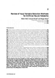
Figure 1: Statistics for short runs for three data sets (simulated data as boxplots, Barley and Pollution data as lines) and 11 variable selection methods. (a) Standardized times to run 1000 MCMC iterations (standardised to have a mean of 1), (b) Estimated effective number of MCMC samples for α (for adaptive shrinkage using Jeffreys’ prior applied to Simulated data and all Pollution results > 150), (c) Total numbers of runs for indicator variables, Priors set 1, (d) Total numbers of runs for indicator variables, Priors set 2. The fixed effect variant of Kuo & Mallick method was not run for the simulated data.

102

4.1

Bayesian Variable Selection Methods

Computational Performance

Summaries of the computational performance of the different methods are plotted in Figure 1. Speedwise, the GVS and Kuo & Mallick methods are slower per iteration than the others, whilst the reversible jump MCMC can be much quicker. The effective number of MCMC samples are all fairly similar, except that the Laplacian shrinkage does less well, and the reversible jump MCMC tends to do better than the other methods. The adaptive shrinkage using Jeffreys’ prior performed much better than the rest of the methods for the simulated data. The number of changes in state of the indicators was generally similar. The fixed effect variants tended to perform poorly, so using a random effects prior (global adaptation) improved the mixing. The effect of the hierarchical variance is to pull the posteriors for the βj ’s towards the right part of the parameter space, so that when Ij = 0, βj is being sampled from close to the correct part of the parameter space. It is interesting that the fixed effect GVS method does not exhibit good mixing.

4.2

Estimation: Simulated Data

The posterior inclusion probabilities of a variable being in a model are plotted against their true values in Fig. 2, and all of the posterior inclusion probabilities are plotted in Fig. 1 of the Supplementary Material. The slope of the fitted line in Fig. 2 indicates how well the method does in distinguishing between important and minor effects, and the position along the x-axis indicates how sensitive the method is to letting smaller effects into the model. The Laplacian models perform poorly, with worse discrimination than the no selection models. The other methods perform similarly to each other, with the exception of the fixed effect GVS with flat priors, which tends to exclude variables, and the Meuwissen & Goddard form of SSVS with informative priors, which behaves inconsistently. The posterior distribution of the variable with the largest true effect size is shown in Fig. 3. The conditional distributions (i.e. P (βj | Ij = 1, data)) are similar: the principal difference being the larger uncertainty in the Laplacian estimates. The figures are similar for the second set of priors (see Fig. 2 in Supplementary Material), except that in the case of the random effects SSVS P (βj | Ij = 0, data) and P (βj | Ij = 1, data) are very similar.

4.3

Estimation: Barley data

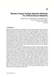
The posterior estimates of P (Ij = 1 | data) from different methods are shown in Fig. 4. For both set of priors, the No Selection and Laplacian shrinkage methods work badly, showing high marginal posterior occupancy probabilities for all loci. In contrast, the

R.B. O’Hara and M. J. Sillanp¨a¨a

Kuo & Mallick

SSVS

1.0

1.0

0.8

0.8

0.8

0.6

0.6

0.6

0.4

0.4

0.4

0.2

0.2

0.2

0.0

0.0 0.2

0.4

0.6

0.0 0.0

0.2

0.4

0.6

1.0

1.0

1.0

1.0

0.8

0.8

0.8

0.8

0.6

0.6

0.6

0.6

0.4

0.4

0.4

0.4

0.2

0.2

0.2

0.2

0.0

0.0

0.0

0.2

0.4

0.6

0.0

0.2

0.4

0.6

1.0

1.0

0.8

0.8

0.8

0.6

0.6

0.6

0.4

0.4

0.4

0.2

0.2

0.2

0.0

0.0 0.2

0.4

0.6

0.6

0.2

0.4

0.6

0.0

0.2

0.4

0.6

Reversible Jump

1.0

0.0

0.4

0.0 0.0

Laplacian

Jeffreys

0.2

SSVS, M & G

Fixed

0.0

0.0

0.0 0.0

0.2

0.4

0.6

0.0

0.2

0.4

0.6

1.0

1.0

1.0

0.8

0.8

0.8

0.6

0.6

0.6

0.4

0.4

0.4

0.2

0.2

0.2

0.0

0.0 0.0

0.2

0.4

0.6

Random

0.0

Fixed

GVS

1.0

Random

No Selection

True Effect Size

103

0.0 0.0

0.2

0.4

0.6

0.0

0.2

0.4

0.6

Pr(Ij=1 | data)

Figure 2: Posterior inclusion probabilities for simulated data plotted against true values of the coefficients. Lines show the fitted curves (quasi-binomial generalized linear model with a logit link). Black and dots: priors set 1, cyan and crosses: priors set 2.

104

Bayesian Variable Selection Methods

Reversible Jump, Random Reversible Jump, Fixed Laplacian, Random Laplacian, Fixed Jeffreys SSVS, M & G SSVS, Random SSVS, Fixed GVS, Random GVS, Fixed Kuo & Mallick, Random No Selection, Random No Selection, Fixed

0

0.0 Reversible Jump, Random Reversible Jump, Fixed Laplacian, Random Laplacian, Fixed Jeffreys SSVS, M & G SSVS, Random SSVS, Fixed GVS, Random GVS, Fixed Kuo & Mallick, Random No Selection, Random No Selection, Fixed

0.03

0.1

0.2

0.3

0.4

0.0

0.1

0.09

0.0

0.1

0.2

Reversible Jump, Random Reversible Jump, Fixed Laplacian, Random Laplacian, Fixed Jeffreys SSVS, M & G SSVS, Random SSVS, Fixed GVS, Random GVS, Fixed Kuo & Mallick, Random No Selection, Random No Selection, Fixed

0.18

Reversible Jump, Random Reversible Jump, Fixed Laplacian, Random Laplacian, Fixed Jeffreys SSVS, M & G SSVS, Random SSVS, Fixed GVS, Random GVS, Fixed Kuo & Mallick, Random No Selection, Random No Selection, Fixed

0.27

0.0

0.0

0.2

0.06

0.2

0.3

−0.10

0.12

0.3

0.4

0.5

0.6

0.7

0.0

0.2

0.4

0.6

0.0

0.21

0.2

0.4

0.6

0.0

0.1

0.00

0.05

0.10

0.15

0.15

0.1

0.2

0.3

0.4

0.5

0.6

0.24

0.2

0.3

0.4

0.5

0.2

0.3

0.4

0.5

0.6

0.0

0.1

0.2

0.3

0.4

0.5

0.3

0.4

0.6

0.8

0.0

0.1

0.6

βj | Ij, data

Figure 3: Posterior distributions for regression coefficients, βj , for the variable with the largest true effect size in the Simulated data, with vague priors. Posterior mode and 70% highest posterior density interval. Black: fixed effect models, cyan: random effect models. Strong colours (i.e. black and red) denote P (βj | Ij = 1, data), Lighter colours (i.e. grey and light cyan) denote P (βj | Ij = 0, data). The dotted line shows the true effect size of the simulated coefficients. Numbers in plots are b in the simulations of the data: a higher number equates to a larger variation in the true coefficients (see text for details).

R.B. O’Hara and M. J. Sillanp¨a¨a

105

Priors 1

Priors 2 No Selection

1.00 0.75 0.50 0.25 0.00

Kuo & Mallick

1.00 0.75 0.50 0.25 0.00 1.00

GVS

0.75 0.50 0.25 0.00

0.75

SSVS

Pr(Ij=1 | data)

1.00

0.50 0.25 0.00

Jeffreys

1.00 0.75 0.50 0.25 0.00

Laplacian

1.00 0.75 0.50 0.25

Reversible Jump

0.00 1.00 0.75 0.50 0.25 0.00 1

2

3

4

5

6

7

1

2

3

4

5

6

7

Chromosome

Figure 4: Posterior inclusion probabilities for Barley data. Dotted line: prior probability, light grey region: 3