Proceedings of IDETC/CIE 2008 ASME 2008 International Design Engineering Technical Conferences & Computers and Information in Engineering Conference August 3-6, 2008, New York City, NY, USA
DETC2008-49411 A REVIEW OF RECENT PHASE TRANSITION SIMULATION METHODS: SADDLE POINT SEARCH Devendra Alhat Department of Metallurgical Engineering & Materials Science Indian Institute of TechnologyBombay, Mumbai 400076, India
Vernet Lasrado Department of Industrial Engineering & Management Systems University of Central Florida Orlando, FL 32816, U.S.A.
transition to occur, one must supply this energy Ea to the reactants so that they can jump over the energy hump and convert to the products. In this sense, first-order phase transition process is similar to reaction. One may write the transition algebraically as Reactant + Ea Æ Product + ΔH where ΔH is the latent heat; thermodynamically known as enthalpy of reaction. In second-order phase transition, there is no latent heat involved. Per the Arrhenius theory, the kinetics of the transition is proportional to exp(− Ea / kT ) , where Ea is the activation energy, k is the Boltzmann constant and T is the temperature. The calculated value of Ea from the atomic or molecular scale can be used as the parameter for a larger scale phase transition simulation such as kinetic Monte Carlo (KMC) simulation [11].
ABSTRACT A review of saddle point search methods on a potential energy surface is presented in this paper. Finding saddle points on a complex potential energy surface is the major challenge in modeling and simulating the kinetics of first-order phase transitions. Once the saddle points have been identified and the activation energy for the transition is known, one can apply the kinetic Monte Carlo method to simulate the transition process. We consider some factors while reviewing the methods, such as whether the solution is global, the knowledge of the Hessian during the search, the capability to locate multiple saddle points and higher order saddle points, the kind of approximations used for potential energy surface, if any; and the convergence of the methods. 1.
INTRODUCTION Phase transition process of materials is a very important part of our daily lives and makes us and our society functional. Functional materials for rechargeable batteries in portable electronics or binary optical or magnetic information storage devices are all based on transition properties. From a broader perspective, atomic diffusion inside solid materials and metabolic processes occurring within our body are also examples of phase transitions. The structures and physical properties of materials between two phases are distinct. Compared to continuous or second-order phase transitions, discontinuous or first-order phase transitions are observed more often. Each phase represents a state of the system with a local minimum of total energy. As illustrated in Fig.1, an activation energy barrier usually exists between the two transforming phases, which is denoted as Ea in the figure. For a phase *
Yan Wang* Department of Industrial Engineering & Management Systems University of Central Florida Orlando, FL 32816, U.S.A. Email:
[email protected]
Fig.1. Energy diagram showing first-order phase transition pathway for single step spontaneous process. Ea is the activation energy barrier. ΔH is the heat of reaction.
All correspondence to this author
1
Copyright © 2008 by ASME
Therefore the most important step involved in the formulation of phase transition simulation is the knowledge of the activation energy barrier involved in the transition. The accuracy of its value determines the accuracy of simulation. The activation energy can be found by exploring the potential energy hyperspace of the reactants and the products and thereby locate the minimum energy path (MEP) or saddle points. Traditionally, the rate of transition is found based on the harmonic transition state theory with quadratic approximation or variational transition state theory (VTST) [2, 3]. Compared to vibrations and other thermal behaviors, phase transitions are rare events. Traditional molecular dynamics (MD) simulation is not efficient. As much as 1012 seconds may be required for sampling pathways to dissociation of an acid with the traditional MD simulation methods. We normally focus on the dynamical bottleneck for the rare event to avoid such a long computational time. In the case of nucleation in a system, for instance, this rare event is the formation of critical nuclei. Once the transition rate is derived, simulation methods such as path sampling [10] or temperature accelerated hyperdynamics [36] can be applied. Other accelerated sampling methods such as umbrella sampling [1] can also be used. More recently, methods to directly search saddle points by exploring potential energy surfaces have been developed. One may generate potential surfaces by using the ab initio calculation [4], analytical parameterization [5], and quantumchemical approximation [6]. One may even approximate the actual potential with the sum-of-squares decomposition of potential energy surfaces [7] or local Taylor approximation [8, 9] to make the numerical methods applicable for computation. Even though the approximations may not be applicable to complex surfaces, they reduce the computational cost with faster convergence. In this paper, we give a review of saddle point searching methods in phase transition simulation, as a continuation of [12] which summarizes minimum energy path searching algorithms. There have been a few survey papers on methods of searching transition path and saddle point [37, 38]. The latest one on saddle point search was published in 2004 by Olsen et al [13]. However, it reviewed mostly the surface walking methods. Here we provide a comprehensive survey of surface walking and other methods developed more recently such as the ridge, the step and slide, the distinguished coordinate and other methods. We intend to make the review as self-contained as possible so that it could be assimilated easily by researchers with different backgrounds.
ended search. These methods include the DHS, the Ridge, the Step and slide, etc. In contrast, others such as the activation relaxation, the dimer, etc. are based on single-ended search. 2.1
Automated Surface walking algorithm (1983) This method was developed by Simons et al. [14] and can be used for finding the local minima as well as a saddle point depending on the eigenvalue being tracked: either positive (corresponds to a minimum) or negative (corresponds to a saddle). Only local information (local gradient and Hessian) is used to walk towards the stationary point. The essence of the walking algorithm is to search iteratively based on a local quadratic approximation of the potential energy surface using second-order Taylor polynomials. Thus the approximation is only valid within a local neighborhood specified by a trust radius. The trust radius is updated in each iteration by the Fletcher approach [15], which is done by comparing the approximate potential energy E (x) and the actual potential energies E ( x) at the position x in the configuration space with reaction coordinates. The ratio of the actual and the approximate energy change of the step xi −1 to
xi is represented as Ω=
E (xi ) − E (xi −1 )
(1) E (xi ) − E (xi −1 ) The ratio of the actual and the approximate energy change represents the fitness of the local approximation to the actual potential energy surface. The closer Ω is to unity, the more quadratic is the true energy surface. The walking step size is constrained to be within the trust radius hi . The algorithm for updating the trust radius and the criteria for the rejection of the current step if carried in wrong direction are listed as follows, where Ω min and Ω max are two thresholds to measure the difference. i. If Ωmin ≤ Ω ≤ Ω good or 2 − Ωmin ≤ Ω ≤ 2 − Ω good , then accept the step from xi −1 to xi and keep the same trust radius hi = hi −1 . ii. If Ω good ≤ Ω ≤ 2 − Ω good , then accept the step from
xi −1 to xi and increase the trust radius hi = α hi −1 , where α > 1 . iii. If Ω < Ω min or Ω > 2 − Ωmin , then the step xi −1 to xi is rejected. Instead a new step is formulated with a decreased trust radius hi = 1/ α hi −1 , where α > 1 . The example potentials tested in [14] showed that the method is insensitive to the choice of Ω min , Ω good and α .
2.
SADDLE POINT SEARCHING METHODS Most of the methods reviewed here rely on a local approximation of the potential energy surface such that the computational cost involved in the iteration decreases. In most of the cases the surface is approximated by a quadratic function. Some of the methods also require both the initial and final states of the system to be known and are based on double-
The Hessian matrix for the method is updated for each iteration using the BFGS update procedure [15] or Powell’s update procedure [16]. However, other update procedures available in numerical analysis literature [15] may also be used. The BFGS update of the Hessian matrix H i +1 at the step (i+1)th is defined as 2
Copyright © 2008 by ASME
H i +1 = H i +
(Fi +1 − Fi )(Fi +1 − Fi )t (Fi +1 − Fi )t (xi +1 − xi )
H (x − x )(x − x )t H i − i i +1 it i +1 i (xi +1 − xi ) H i (xi +1 − xi )
Reference [17] describes the application of this method to simulation of Cope and Claisen rearrangement of organic molecules.
(2)
2.3
The partitioned rational function optimization (RFO) method (1985) This method developed by Banerjee et al. [18] is a local saddle point search algorithm, which is based on local rational function approximation to the potential surface with augmented Hessian, as in gt x + 0.5xt Hx E ( x) − E ( x) = (5) 1 + xt Sx
where (Fi +1 − Fi ) is the forward force difference, and the force is defined by the gradient of potential as F = −∇E . Comparatively, the Powell’s update scheme is defined as ΔH iPowell = (Δg i +1 − H i ⋅ Δx i ) ⋅ Δxti + Δxi ⋅ (Δg i +1 − H i ⋅ Δxi )t Δxti ⋅ Δxi −(Δg i +1 − H i ⋅ Δxi )t ⋅ Δx i
(3)
where E (x) is the approximate to the energy E (x) , x is the step vector, g is the gradient vector described by equation (4), H is the Hessian, S is a diagonal scaling matrix. Reference [18] claims that the convergence of the method to the saddle point is quadratic as opposed to linear for most of the other methods. The method may be further classified as: RFO using exact Hessian to the systems for which the exact Hessian is known, and RFO with approximated Hessian for systems where the calculation of Hessian is laborious. The simplest starting approximation for the initial Hessian is the identity matrix. The Hessian is updated for the (i+1) iteration as, H i +1 = H i + ΔH i where ΔH i is generated either using Powell’s Hessian updating procedure [16] or Bofill’s Hessian [19] updating procedure. The Powell’s update scheme is represented by Equation (3). The Bofill update scheme is represented by (6) ΔHiBofill = φ Bofill ΔHiSR1 + (1 − φ Bofill )ΔHiPowell
Δx i ⋅ Δxi t ( Δx i t ⋅ Δx i ) 2
where g is the gradient vector with Δg i +1 = g(xi +1 ) − g(xi )
(4)
The Powell’s scheme preserves the Hermitian character of the updated matrix ( H i +1 ). One may use the identity matrix as the initial Hessian. The automated surface walking algorithm also involves the scaling of one of the active coordinates in order to make the eigenvalues of the Hessian lie in a required range, depending on whether one is finding a local minima or a saddle point. Reference [14] describes how this method can be applied to simulate the transition of HCN from ground to excited state. To summarize, the algorithm starts with the initial guess of the Hessian either based on the force characteristics of local minimum energy geometry or by approximating the Hessian with the identity matrix. Then, the search starts by tracking the eigenvalue of the updated Hessian at each step till the convergence is reached.
where (Δg i +1 − H i ⋅ Δxi ) ⋅ (Δg i +1 − H i ⋅ Δxi )t (Δg i +1 − H i ⋅ Δxi )t ⋅ Δxi is a symmetric and rank one matrix update and ΔH iSR1 =
2.2
DHS Method (1984) This method developed by Dewar et al [17] is an efficient method for finding the region of the saddle point on less complicated potential energy surfaces. In the configuration space, each configuration is called an image. Essentially, the main idea of this method is to pull the lower energy image over the potential energy surface towards the higher energy image. At a certain point along this movement of the lower energy image, the saddle point is crossed, which can be checked via the optimization step. Initially, one needs to determine the reactant and product, and join the two by a line. Each of these geometries forms an image in the high dimensional configuration space with reaction coordinates. For each iteration, the energy of both the images is calculated and the lower energy image is pulled towards the higher energy image along the line segment connecting the two images. This is obtained by reducing the distance between the images by a factor of 5%, keeping the higher energy image fixed. The lower energy image is the minimized keeping the newly computed reduced distance between the fixed images. If the distance between the images is sufficiently small, the iteration is terminated.
φ Bofill =
[(Δg i +1 − H i ⋅ Δxi )t ⋅ Δxi ]2 [( Δg i +1 − H i ⋅ Δxi )t .(Δg i +1 − H i ⋅ Δxi )](Δxi t ⋅ Δxi )
is a Bofill factor. Partitioned rational functions rather than rational functions are used for ease of implementation in finding saddle points. The difference between the rational function optimization and the partitioned rational function method is that in partitioned RFO with a μ th order saddle point, one performs energy maximization along μ chosen principal modes corresponding to μ smallest eigenvalues of the Hessian and minimization along the remaining (n − μ ) principal modes. The RFO matrix is partitioned as follows: g1 ⎞ ⎛ x1 ⎞ 0 0 ⎛ H1 ⎛ x1 ⎞ ⎜ ⎟⎜ ⎟ ⎜ ⎟ 0 0 ⎜ ⎟⎜ ⎟ = λ ⎜ ⎟ (7) p ⎜ ⎜ 0 0 H μ g μ ⎟ ⎜ xμ ⎟ xμ ⎟ ⎜ ⎟⎜ ⎟ ⎜ ⎟ ⎜ g1 ⎜1⎟ gμ 0 ⎟⎠ ⎜⎝ 1 ⎟⎠ ⎝ ⎝ ⎠
3
Copyright © 2008 by ASME
⎛ H μ +1 ⎜ ⎜ ⎜ H n, μ +1 ⎜ ⎜ g μ +1 ⎝
H μ +1, n Hn gn
g μ +1 ⎞ ⎛ xμ +1 ⎞ ⎛ xμ +1 ⎞ ⎟⎜ ⎟ ⎜ ⎟ ⎟⎜ ⎟=λ ⎜ ⎟ n ⎜ g n ⎟ ⎜ xn ⎟ xn ⎟ ⎟⎜ ⎟ ⎜ ⎟ ⎜ 1 ⎟ 0 ⎟⎠ ⎜⎝ 1 ⎟⎠ ⎝ ⎠
clusters, which can be described very well in configurational space. However, it is difficult to describe or represent these complex systems in real space. ART does not require any initial guess. It just needs the potential energy surface. To reach the saddle point the method involves the displacement of the configuration in such a way that forces are minimized along all directions except one which corresponds to the lowest eigenvalue. The algorithm essentially consists of three parts: escaping the starting local minimum, convergence to the saddle point and relaxation to the minimum. For escaping the minimum, one needs to take a small random displacement away from the minimum as a first step. Authors of [21] recommended following the direction along the force induced by a small random displacement for escaping the minimum. This direction is followed until the threshold of escape is reached, which is indicated by either force component parallel to the displacement becoming constant or the ratio of this parallel force component to the perpendicular component becoming smaller than a given fraction. Once this harmonic region is left, the process of convergence to saddle point begins by following the direction of a modified force vector G as (9) G = F − (1 + α )(F ⋅ r )r
(8)
where λ p is the highest eigenvalue and is always positive and
λn is the lowest eigenvalue which is always negative. Once the RFO matrix is formulated, one needs to calculate only the lowest eigenvalue of the matrix, which defines the new starting point for the next iteration. Soft mode and stiff mode can be chosen to walk depending on the direction. This process is continued till convergence where λ p and λn both become zeros. 2.4
Ridge Method (1993) This method was developed by Ionova and Carter [20]. It is a surface walking algorithm and does not involve the use of Hessian. Hence, this method can be used for systems where the computation of Hessian is difficult. The initial guess for transition state geometry is not required. It starts searching for a maximum on the linear path connecting reactants and products, and the search is solely based on local information. As a result, it may lead to a path that is different from MEP if the search is initiated far from the MEP. Once the maximum energy point along the initial linear path is found, two images around that point on the same initial linear path are formed and separated by a certain distance. These two images are then displaced individually towards down-hill directions. In the next iteration, a maximum along the line joining the two images at the new locations is searched. The line joining the two images is always kept in the direction of negative curvature in each iteration. This procedure of displacing and searching for maximum along the line is continued till the saddle point is reached, where the curvature becomes zero. It is important to note that one can also impose linear constraints on the system modeled by the ridge method, as discussed in [20], such that the certain coordinates are frozen or the center of mass of the images is fixed. The ridge method does not guarantee that the saddle point obtained is global. Reference [20] describes how the ridge algorithm can be successfully applied to the simulation of decomposition of disilane.
where F is the total force on the configuration which is calculated using the interaction potential, α is the control parameter, r is a displacement vector from current position ( x ) to the local minimum ( m ), i.e. r = x − m , and r is the normalized vector of r . It is important to note that G cannot be generated using gradient of a scalar, so we cannot use standard minimization techniques here. The convergence to the saddle point will be indicated by the change of sign of the force component parallel to the displacement. The step size is (10) Δx = (H −1 )F with H = Hl + β I ; where H l is the local Hessian, I is the identity matrix, and β is another control parameter. Once the saddle point is reached, it just remains to relax the configuration down the gradient to another local minimum. This is a very stable process and many minimization algorithms can guarantee the convergence. However, authors of [21] recommend that one should use the same algorithm described above to descent down as well. Since this algorithm follows a single eigenvector, it cannot be used to find second or higher order transition states. Reference [21] describes the application of ART to simulation of amorphous silicon and silica glass. The configuration of the atoms at saddle point of transition has been successfully obtained using this technique.
2.5
Activation-Relaxation Technique (ART) (1998) The activation-relaxation technique was developed by Mousseau and Barkema [21]. The method is based on a 2-step process called “event”. In the first step a configuration (system) is activated from a local minimum to a saddle point and then relaxed from that saddle point down-hill to another minimum. This method can track a certain fraction of saddle points depending on the implementation and the system. This method uses 3N-dimensional configurational space to model the moves of atoms. This method can be applied very well to the glassy and amorphous materials, polymers, semiconductors and
2.6
Dimer Method (1999) This method originally developed by Henkelman and Jónsson [22] is a minimum-mode (curvature) following saddle point search algorithm. This method can be used when the final state of the transition is not known and does not require the knowledge of the Hessian matrix. This method does not
4
Copyright © 2008 by ASME
(referred as two replicas). The replicas traverse from the isoenergetic surfaces lying below the saddle point to higher isoenergetic surfaces and eventually converge to the saddle point by bracketing the potential. The stepping part involves placing each replica on a specified isoenergetic surface, while the sliding part involves each replica sliding on its respective isoenergetic surface until the distance between the replicas is minimized. The images are pulled towards each other with distance minimization between the replicas on isoenergetic surfaces. The replicas on either side of the saddle point will eventually converge to the saddle point as the potential approaches the transition state. This distance minimization step avoids the problem of one replica jumping over to the other potential well when it is close to the saddle point. After each minimization, the saddle point is bracketed. This bracketing is used to monitor convergence, with an upper bound (the maximum potential on the line connecting the two replicas) and a lower bound (the current potential, i.e. the potential as described by the isoenergetic surface the replica is on). The procedure is repeated by moving to a higher isoenergetic surface until a saddle point is reached. However one must proceed with caution. If the step size is too high, the replicas may move to an isoenergetic surface above the saddle point. This can be checked by calculating the force at the point where the replicas meet. If the force is greater than zero, we have stepped above the saddle point. Essentially, two images climb the mountain separating the initial and final states and meet at the saddle point. The method can also be applied for probing complex potential surfaces with many minima and saddle points. In the event of multiple minima, a minimal bracketing with no intermediate potential minima for each saddle point should be found. The procedure should be restarted with the initial position in the closest set of minima. Reference [24] describes the application of this method to study diffusion mechanisms of a small Ag cluster on a Ag(111) surface using an embedded-atom method potential.
evaluate the complete Hessian. Rather, it evaluates the lowest eigenvalue and the corresponding eigenvector. This method considers a pair of two images of the system, called dimer, and minimizes the energy using rotation and translation at the center of the dimer iteratively. The curvature at the dimer midpoint is given by C=
E − (2 E0 ) ( ΔR )
2
(11)
where E is the energy of the dimer, E0 is energy at dimer midpoint and ΔR is the distance from the dimer midpoint to the dimer end point. Eq.(11) reveals that the minimization of the curvature implies the minimization of the dimer energy. The rotation of the dimer is made in such a way so as to minimize the curvature, thereby minimizing the energy. In the last step of the iteration the dimer is translated by application of a force, depending on the curvature, so as to bring the dimer to the saddle point. One may use either the Newton’s method or the conjugate gradient method for rotation and either the quickmin or the conjugate gradient for dimer translation. Reference [22] quotes an example where dimer method is used to study the transition mechanisms for diffusion of an Al adatom on Al(100) surface. The study was aimed at finding the mechanism by which the diffusion occurs. 2.7
Improved Dimer Method (2005) This method is an improvement by Heyden et al [23] to the Dimer method [22]. The original Dimer performs well on an analytical potential energy surface, but performs significantly poorly when applied to the quantum-chemical potential surface, where the forces are subject to a large amount of numerical noise. The improved method is based on the fact that reducing the number of gradient calculations per cycle from six to four gradients or three gradients will significantly improve the overall performance of the dimer algorithm on quantumchemical potential energy surfaces. This improved method uses a larger rotation step than the original Dimer method for exploring the quantum-chemical potential energy surfaces. Also it uses steepest descent method for rotation calculations rather than the conjugate gradient method. It uses the conjugate gradient for translation of dimer. Instead of performing the gradient calculation at one of the images, it is done at the dimer midpoint, and the gradient at the image is approximated by a linear function. This decreases the accuracy of the curvature calculation in Eq.(11) from O(ΔR 2 ) to O(ΔR ) . It also decreases the number of gradient calculations. Reference [23] discusses various examples where the improved dimer converges more efficiently for systems where the forces are subject to numerical noise than the original dimer method. It also gives a flow chart of the algorithm for the improved Dimer method.
2.9
Concerted Variational Strategy (2003) This method was developed by Passerone et al. [25]. It uses variational principles of classical mechanics to generate a transition path connecting the reactant and the product. This technique is based on the Hamilton principle, which states that every classical trajectory that starts from a configuration qA and renders the action ends in qB after a time period τ stationary, and the Maupertuis principle, which gives the path followed by the system without the specification of the time parameterization of the path. The method can be used for large systems. Starting with any two points qA and qB which lie in two potential basins, a linear interpolation is constructed joining them. Further, a rough approximation to the MEP is generated using inverted potential in
2.8
Step and Slide Method (2001) This method was originally developed by Miron and Fichthorn [24]. The initial and final states must be known
5
Copyright © 2008 by ASME
⎛ 1 ⎛ q (l +1) − q(l ) ⎞2 ⎞ − E (q(l ) ) ⎟ S H := Δ ∑ ⎜ m ⎜ ⎟ ⎟ Δ l =1 ⎜ 2 ⎝ ⎠ ⎝ ⎠ P −1
from the linear interpolation is adjusted so as to minimize the objective function: (r (cc) − rab (ii )) 2 Θ = ∑ ab + (rab (i )) 4 a ≠b
(12)
where, S H is called as a discretized “action” of Hamilton’s
10−6
principle with the integral substituted by a sum, q(t) is a dynamical path, m is the mass, P is the number of points on the mesh and Δ is the time step (Δ = τ / P) . Once the rough estimate of the MEP is obtained, a nonuniform time distribution is calculated using dqi dqi ds ds i =1 ds 2( Etot − E )
w= x, y , z a
τ =∫ 0
∑m
i
(13)
SM = ∫ 0
1 2 ∑ (r (cc) − (rab + R (ii)) ζ ((rab+ R (ii)) + 10−6 ∑a (wa (cc) − wa (ii))2 2 a ,b , R ab + R
(14)
where ζ ((rab (ii)) =0
Once the updated τ is obtained one needs to go back to the Hamilton’s principle in Eq.(12) and iterate till convergence is reached. Then the conjugate residual method [26] for local search is used to find the saddle point of SH. The most important part of this method is energy conservation, which is the most critical requirement for this method to converge most efficiently and in a numerically stable way to a path that is very close to the dynamical path. Reference [25] describes the successful application of this method to the configurational transition of alanine dipeptide molecule. In this study, the authors have condensed the molecule except the atoms involved the transition into “superparticles” in accordance with united atom scheme.
:a=b
ζ ((rab + R (ii )) =
1 (rab + R (ii )) 4
ζ ((rab + R (ii )) =
1 1 − 4 (rab + R (ii )) 4 rcut
ζ ((rab + R (ii )) = 0
: a ≠ b, R = 0 : rab + R (cc ) < rcut a ≠ b, R ≠ 0 : rab + R (cc ) > rcut
Here, a and b are taken for all atoms in a unit cell; R is the real space lattice vectors and rcut is chosen such that R spans a few unit cells. Reference [27] describes the successful application of the method to the Woodward-Hoffmann allowed disrotatory interconversion of the cyclopropyl and ally1 cations and conrotatory interconversion of cyclobutene and cis-butadiene.
2.10 Synchronous Transit Method (2003) The original synchronous transit method was proposed by Halgren and Lipscomb [27]. This method can be used to find the first order saddle points. The linear synchronous transit (LST) generates idealized structures using linear interpolation of distance between two limiting structures that are reactant and product, whereas the quadratic synchronous transit (QST) deals with quadratic interpolation formed by three points: initial state, final state, and an estimate of transition state. The interpolation formula for the LST can be represented as: (15) rabi ( f ) = (1 − f )rabR − frabP R
(16)
Θ( f ) =
3N
σ
2
a
LST maximum estimate may be further improved using orthogonal constraint optimization described in [27]. The method may be summarized as a single line minimization of energy in the direction orthogonal to the LST path, which is followed by the energy maximization along the QST path. An improvement to this method was proposed by Govind et al [28]. The new method is a combination of LST and QST with conjugate gradient refinement for periodic systems, where the objective function needs to be modified. The modified objective function is
where Etot is the total energy, E is the potential energy and q(0) = q A and q(σ ) = q B are two end points parameterized by σ in the spatial domain for the Maupertuis action, which is SM described by Eq.(14). For a system of N particles, with 3N degrees of freedom of mass mi, the Maupertuis action is dq dq mi i i ∑ ds ds ds 2( Etot − E ) i =1 2( Etot − E )
a
where, (cc) and (ii) denote calculated and interpolated quantities and wa is the Cartesian coordinate of the atom. The
3N
σ
∑ ∑ (w (cc) − w (ii))
2.11 Reduced Gradient Following (RGF) Method (1998) This method was developed by Quapp et al [29]. The method is an adaptation of the distinguished coordinate method [30-32], which essentially prescribes forcing some coordinates to have a null gradient by means of which a path can be generated. The RGH method is based on generating and following a curve connecting the saddle point(s) to the extremes, i.e. initial, final and intermediates states, if they exist. This curve is not the MEP, although it may follow the reaction coordinate for some examples. The curve is characterized by the shape of PES and the gradient vector between the different states. A stationary point is always one of the intersections of
P
where rab and rab are the inter-nuclear distances between the atoms a and b in reactant and product respectively and f is an interpolation parameter. The QST uses a similar equation except that the equation is quadratic in f . The path obtained
6
Copyright © 2008 by ASME
curves that satisfy the (N-1) equations ∂E ( x(t )) =0 i = 1,… , k ,… , N (17) ∂xi in N-dimensional space, where E(x(t)) is the function of the potential energy surface defined by the coordinates x with the parameter t. The starting direction of the search must be chosen carefully. It is usually the initial state of the transition. Every iteration of RGF involves two steps: If Eq.(17) is satisfied with a given tolerance ε, a predictor step is executed. Otherwise, a corrector step is executed. The algorithm is terminated when some stopping criteria are met. The authors suggest determining the step length of a hypothetical Newton step to the next stationary point. If this step length is less than a certain level, the algorithm is terminated as the stationary points are connected. The predictor step is given by: s xm +1 = xm + xm′ (18) xm′
tangent vector to the RGF curve, s is the step length of the former prediction step, and τ is the step vector. The solution to Eq.(20) is thus the combined predictor-corrector step with step length s in the direction of t which is essentially a NewtonRaphson like step. As a result, the predictor-corrector strategy follows the curve generated by Eq.(17) more closely thus reducing the number of calls to the corrector step. As in the original RGF method, every iteration of RGF involves two steps: If Eq.(17) is satisfied with a given tolerance ε, a predictor step is executed. Otherwise, a corrector step is executed. The algorithm is terminated when some stopping criteria are met. Essentially, the predictor step in the original RGF method is modified to include a portion of the corrector step as shown in Eq.(20). As a result, the computationally expensive corrector step is called less often since the prediction error is usually less than the threshold, hence improving the efficacy of the RGF method. The authors also suggest use of Bofill’s update [19] to the Hessian matrix to improve the efficiency of the improved RGF method. Reference [34] depicts the application of this method to the isomerization of butane and ring opening of sym-tetrazine.
where, s is the step length, xm′ is the tangent to the curve given by the solution of d ∂E ( x(t )) = 0 = Hx′ i = 1,… , k ,… , N (19) dt ∂xi where, H is the Hessian matrix, that is updated using the Davidson-Fletcher-Powell update procedure [33]. The corrector step involves a Newton-Raphson like method to solve the systems of equations in Eq.(17) to get the corrected point. This step is computationally expensive. Once the corrected point is obtained, the predictor step is applied again. Essentially, this method fixes one parameter while minimizing the other parameters with respect to the energy for each parameter. Eq.(17) generates (N-1) one dimensional curves that intersect at the saddle point(s) and other stationary points. However, in the event of multiple saddle points, this method does not predict which saddle point(s) will be found. Reference [29] describes the application of this method to simulation of various chemical reactions like HCN to CNH isomerization and Azidotetrazole isomerization to map the geometries at the saddle point.
2.13 Reduced Potential Energy Surface Model (2000) This method developed by Anglada et al. [35] is also an adaptation of the distinguished coordinate method [30-32]. However, as opposed to the RGF method [29, 34], the authors propose a distinguished coordinate method implemented as a steepest ascent path from reactant or products to the transition state. The path generated is not the MEP. The geometric parameters are partitioned into two subsets, br and bp, where br is the subset of parameters exhibiting the largest changes in internal coordinates during transition, while bp includes the rest of the parameters. The saddle point searching is based on a reduced surface with the dimensions of the subset br instead of the original PES, since the stationary points on the reduced surface are also the stationary points on the full surface. To initialize the model, the br parameters are perturbed and optimized, as a result we have the initial geometry, gradient vector and Hessian matrix. Using a variation of the rational function optimization (RFO) method [18], where the authors suggest the use of BFGS method [15] to update the entire Hessian matrix as opposed to the partial Hessian update as prescribed by RFO, the authors minimize the energy with respect to bp, while keeping the br parameters fixed. This results in a new set of parameters br and bp, the gradient and Hessian matrix. At any position, if the norm of the gradient is less than a certain threshold; the authors infer that the point is at a possible transition state. Otherwise, the minimization step is repeated till the convergence criterion is met. Reference [35] describe the application of this method to various simulations like thermal rearrangement of cyclopropyl radical to allyl radical, rearrangement of the methoxy radical to hydroxymethylene radical, the oxidation of the methoxy radical by molecular oxygen forming formaldehyde and hydroperoxy
2.12 Improved Reduced Gradient Following (RGF) Method (2002) This method was developed by Hirsch and Quapp [34] as an improvement to [29]. In the original RGF method, the corrector step is called often as a result of the predictor step going wrong. The improved RGF uses an implied corrector step for each predictor step as a measure of improving the estimates with almost no additional computational effort. The new predictor-corrector step is given by: H (x m +1 ) τ m +1 = g (x m +1 ) (20) t (x m +1 )T τ m +1 = s m where H(x) is the Hessian of the potential energy surface, g(x) is the gradient of the potential energy surface, t(x) is the unit
7
Copyright © 2008 by ASME
radical, etc.
[5] Schatz, G.C. (1989) The analytical representation of electronic potential-energy surfaces. Reviews of Modern Physics, 61(3): 669-688 [6] Brenner, D.W. and Bean, C. P. (1990) Empirical potential for hydrocarbons for use in simulating the chemical vapor deposition of diamond films. Physical review B, 42(15): 9458-9471 [7] Burke, M. and Yaliraki, S.N. (2005) Sum of squares decompositions of potential energy surfaces. arXiv eprint (arXiv:cond-mat/0508293v1) [8] Thompson, K.C., Jordan, M.J.T., and Collins, M.A. (1998) Molecular potential energy surfaces by interpolation in Cartesian coordinates. The Journal of Chemical Physics, 108(2): 564-578 [9] Cerjan, C.J. and Miller, W.H. (1981) On finding transition states. Journal of Chem. Phys., 75(6): 2800-2806 [10] Bolhuis, P.G., Chandler, D., Dellago, C., and Geissler, P.L. (2002) Transition Path Sampling: Throwing Ropes Over Rough Mountain Passes, in the Dark. Annu. Rev. Phys. Chem., 53:291-318 [11] Zhdanov, V.P. (1994) First-order kinetic phase transitions in simple reactions on solid surfaces: Nucleation and growth of the stable phase. Physical Review E, 50(2):760763 [12] Lasrado, V., Alhat, D., and Wang, Y. (2008) A Review of Phase Transition Simulation: Transition Path Search Methods. Proc. ASME IDETC/CIE08, paper No. DETC2008-49410 [13] Olsen, R. A., Kroes, G. J., Henkelman, G., Arnaldsson, A., and Jónsson, H. (2004) Comparison of methods for finding saddle points without knowledge of the final states. J. Chem. Phys., 121(20): 9776-9792 [14] Simons, J., Joergensen, P., Taylor, H., and Ozment, J. (1983) Walking on Potential Energy Surfaces. J. Phys. Chem., 87: 2745- 2753 [15] Fletcher, R. (1980) Practical Methods of Optimization. Vol. 1, Wiley, New York [16] Powell, M.J.D. (1971) Recent Advances in Unconstrained Optimization. Math. Prog., 1: 26-57 [17] Dewar, M.J.S., Healy, E.F., and Stewart, J.J.P. (1984) Location of Transition States in Reaction Mechanisms. J. Chem. Soc., Faraday Trans., 2(80): 227 [18] Banerjee, A., Adams, N., Simons, J., and Shepard, R. (1985) Search for Stationary Points on Surfaces. J. Phys. Chem., 89: 52-57 [19] Bofill, J.M. (1994) Updated Hessian matrix and the restricted step method for locating transition structures. Journal of Computational Chemistry, 15(1): 1-11 [20] Ionova, I.V. and Carter, E.A. (1993) Ridge method for finding saddle points on potential energy surfaces. J. Chem. Phys., 98: 6377-6386 [21] Mousseau, N. and Barkema, G.T. (1998) Traveling through potential energy landscapes of disordered materials: The activation-relaxation technique. Physical Review E, 57(2): 2419-2424
3.
CONCLUSION Various methods for finding the saddle point for phase transition simulation were reviewed in this paper. We can classify the methods as double ended search and single ended search. Double ended search requires both initial and final states of the process to be known, whereas the single ended search involves only one of the two states to be known prior to the start of the simulation. The double ended search includes the DHS, the Ridge, the Step and slide, etc. whereas others such as the activation relaxation, the dimer, etc. are based on single-ended search. The key to the efficiency of the algorithms reviewed is the optimization methods used. The efficacy is determined by the global scope of the algorithm, i.e. the ability to find multiple transitions. Our goal is to provide basic overview for a variety of methods, ranging from the classical to the latest methods. The convergence of most of the methods depends on the good initial guess of the path or the starting point of the search. In the event of a bad initial guess, the methods may converge to a wrong saddle point. Another general trend observed in the survey was that Hessian updating as in quasi-Newton methods has been widely accepted to reduce the computational cost. Most of the surveyed methods rely on an inbuilt assumption that the potential energy surface is perfectly modeled. Yet it should be realized that one important source of simulation errors of phase transitions may be the errors in the potential surface generation itself. ACKNOWLEDGEMENT This work is supported in part by the NSF grant CMMI0645070.
REFERENCES
[1] Frenkel, D. and Smit, B. (1996) Understanding Molecular Simulation: From Algorithms to Applications. Academic Press, San Diego [2] Truhla, D.G., Hase, W.L., and Hynes, J.T. (1983) Current Status of Transition-State Theory. The Journal of physical Chemistry, 87(15): 2664-2682 [3] Hu, W.-P., Liu, Y.-P., and Truhlar, D.G. (1994) Variational Transition-state Theory and Semiclassical Tunnelling Calculations with Interpolated Corrections: A New Approach to Interfacing Electronic Structure Theory and Dynamics for Organic Reactions. J. Chem. Faraday Trans., 90(12): 1715-1725 [4] Hollebeek, T., Ho, T.-S., and Rabitz, H. (1999) Constructing multidimensional molecular potential energy surfaces from ab initio data. Annual review of Physical Chemistry, 50: 537-570
8
Copyright © 2008 by ASME
[22] Henkelman, G. and Jónsson, H. (1999) A dimer method for finding saddle points on high dimensional potential surfaces using only first derivatives. J. Chem. Phys., 111(15): 7010-7022 [23] Heyden, A., Bell, A.T., and Keil, F.J. (2005) Efficient methods for finding transition states in chemical reactions: Comparison of improved dimer method and partitioned rational function optimization method. J. Chem. Phys., 123: 224101-224114 [24] Miron, R.A. and Fichthorn, K.A. (2001) The Step and Slide method for finding saddle points on multidimensional potential surfaces. J. Chem. Physics, 115(19): 8742-8747 [25] Passerone, D., Ceccarelli, M., and Parrinello, M. (2003) A concerted variational strategy for investigating rare events. J. Chem. Phys., 118(5): 2025-2032 [26] Saad, Y. (2003) Iterative Methods for Sparse Linear Systems, 2nd ed., SIAM, Boston [27] Halgren, T.A. and Lipscomb, W.N. (1977) The synchronous-transit method for determining reaction pathways and locating molecular transition states. Chemical Physics Letters, 49(2): 225-232 [28] Govind, N., Petersen, M., Fitzgerald, G., King-Smith, D., and Andzelm, J. (2003) A generalized synchronous transit method for transition state location. Computational Materials Science, 28: 250–258 [29] Quapp, W., Hirsch, M., Imig, O., and Heidrich, D. (1998) Searching for Saddle Points of a Potential Energy Surface by Following a Reduced Gradient. J Comput Chem, 19: 1087-1100 [30] Rothman, M.J. and Lohr, L.L. (1980) Analysis of an energy minimization method for locating transition states on potential energy hypersurfaces. Chem. Phys. Lett., 70(2): 405-409 [31] Scharfenberg, P. (1981) Theoretical analysis of constrained minimum energy paths. Chem. Phys. Lett., 79(1): 115-117 [32] Scharfenberg, P. (1982) An improved method for the evaluation of transition states. J Comput Chem, 3: 277-282 [33] Heidrich, D., Kliesch, W., and Quapp, W. (1991) Properties of Chemically Interesting Potential Energy Surfaces. Springer, Berlin [34] Hirsch, M. and Quapp, W. (2002) Improved RGF Method to Find Saddle Points. J. Comput. Chem., 23: 887-894 [35] Anglada, J.M., Besalú, E., Bofill, J.M., and Crehuet, R. (2001) On the Quadratic Reaction Path Evaluated in a Reduced Potential Energy Surface Model and the Problem to locate Transition States. J. Comput. Chem., 22: 387-406 [36] Rørensen, M.R. and Voter, A.F. (2000) Temperatureaccelerated dynamics for simulation of infrequent events. J. Chem. Phys., 112(21): 9599-9606 [37] Henkelman, G., Jóhannesson, G., and Jónsson, H. (2002) Methods for finding saddle points and minimum energy paths. In Progress in Theoretical Chemistry and Physics,
ed. by W.N. Lipscomb, I. Prigogine, and S.D. Schwartz, Springer, Dordrecht, 269-302 [38] Schlegel, H.B. (2003) Exploring potential energy surfaces for chemical reactions: An overview of some practical methods. J. Comput. Chem., 24(12): 1514-1527
9
Copyright © 2008 by ASME