A Review of Temporal Data Visualizations Based on ... - HAL-Inria

A Review of Temporal Data Visualizations Based on Space-Time Cube Operations Benjamin Bach, Pierre Dragicevic, Daniel Archambault, Christophe Hurter, Sheelagh Carpendale

To cite this version: Benjamin Bach, Pierre Dragicevic, Daniel Archambault, Christophe Hurter, Sheelagh Carpendale. A Review of Temporal Data Visualizations Based on Space-Time Cube Operations. Eurographics Conference on Visualization, Jun 2014, Swansea, Wales, United Kingdom. 2014.

HAL Id: hal-01006140 https://hal.inria.fr/hal-01006140 Submitted on 25 Jun 2014

HAL is a multi-disciplinary open access archive for the deposit and dissemination of scientific research documents, whether they are published or not. The documents may come from teaching and research institutions in France or abroad, or from public or private research centers.

L’archive ouverte pluridisciplinaire HAL, est destinée au dépôt et à la diffusion de documents scientifiques de niveau recherche, publiés ou non, émanant des établissements d’enseignement et de recherche fran¸cais ou étrangers, des laboratoires publics ou privés.

Eurographics Conference on Visualization (EuroVis) (2014), pp. 1–19 R. Borgo, R. Maciejewski, and I. Viola (Editors)

A Review of Temporal Data Visualizations Based on Space-Time Cube Operations B. Bach1 , P. Dragicevic1 , D. Archambault2 , C. Hurter3 and S. Carpendale4 1 INRIA,

France University, UK 3 ENAC, France 4 University of Calgary, Canada 2 Swansea

Abstract We review a range of temporal data visualization techniques through a new lens, by describing them as series of operations performed on a conceptual space-time cube. These operations include extracting subparts of a space-time cube, flattening it across space or time, or transforming the cube’s geometry or content. We introduce a taxonomy of elementary space-time cube operations, and explain how they can be combined to turn a three-dimensional space-time cube into an easily-readable two-dimensional visualization. Our model captures most visualizations showing two or more data dimensions in addition to time, such as geotemporal visualizations, dynamic networks, time-evolving scatterplots, or videos. We finally review interactive systems that support a range of operations. By introducing this conceptual framework we hope to facilitate the description, criticism and comparison of existing temporal data visualizations, as well as encourage the exploration of new techniques and systems. Categories and Subject Descriptors (according to ACM CCS): H.5.0 [Information Systems]: Information Interfaces and Presentation—General

1. Introduction Temporal datasets are ubiquitous but notoriously hard to visualize, especially rich datasets that involve more than one dimension in addition to time.

isting techniques by their name, both for general visualizations [Har99] and for temporal visualizations [AMST11].

Previous work on novel visualizations for temporal data has dramatically advanced the field of information visualization (infovis). However, there are so many different techniques today that it has become hard for both researchers and designers to get a clear picture of what has been done, and how much of the design space of temporal data visualizations remains to be explored. For similar reasons, teaching this research topic to students is challenging. Therefore, there is a clear need to structure and organize previous work in the area of temporal data visualization.

Although names are essential for indexing, retrieval and communication purposes, they are a poor thinking tool. Because there is no convention for naming techniques, names rarely reflect the essential concepts behind a technique. For example, names such as Value Flow Maps [AA04b] and Planning Polygons [SRdJ05] say little about the possible conceptual similarities between the two techniques (see Figure 1). Names can also be ambiguous. For example, the term small multiples is commonly used to refer to a specific type of temporal data visualization [Tuf86]. But Figure 2 shows that two visualizations can be based on small multiples despite being very different conceptually.

Part of the problem is that information visualization researchers have mostly focused on nomenclature. Most familiar charts have an agreed-upon name, e.g., bar charts or scatter plots, and this tradition has been continued in infovis, where each newly published visualization technique is given a different name. Many textbooks and surveys list ex-

There has been recent effort at proposing taxonomies, conceptual models and design spaces for temporal visualizations, mainly focusing on analytical tasks and data types (e.g., object movement data [AAH11, AAB∗ 11, AA12], video data [BCD∗ 12], or datasets with different temporal and spatial structures [AMM∗ 07]).

submitted to Eurographics Conference on Visualization (EuroVis) (2014)

2

B. Bach & P. Dragicevic / A Review of Temporal Data VisualizationsBased on Space-Time Cube Operations

(a) Value flow diagram [AA04b]

Figure 3: A space-time cube based on an illustration by Hägerstrand [Hä70] in 1970, showing social interactions across space and time.

(b) Planning Polygons [SRdJ05]

Inflation (%)

-2

0

2 0

10 20 Unemployment rate (%)

France

8 6 4

90 92 96 94 98

2

-2

90 92 94 98 96 00 0

Spain

8

90

4

00

2

98

00 0 -2

0

92

6

94 96

0


-2

0


(a) By country

4

6 4

2

2

0

0 0

1996

8

-2


6 4

0 0


-2

4

-2


1998

4 2

6

0 0

6

0

1994

8

2

8

2

-2

1992

8

Inflation (%)

6

-2


1990

8

Inflation (%)

4

Inflation (%)

0

6

Inflation (%)

00 92 98 96 94

2

Japan

8

Inflation (%)

90

4

Inflation (%)

6

Inflation (%)

USA

8

Inflation (%)

Inflation (%)

Figure 1: Two conceptually similar temporal visualization techniques showing: (a) the evolution of crime statistics in every US state; (b) the evolution of high school population in several districts across 3 years.

0


2000

8 6

The term space-time cube originates from cartography, where it refers to a geographical representation where time is treated as a third dimension [AA03]. One of the earliest uses was by geographer Hägerstand in 1970, who described a "space-time model which could help us to develop a kind of socio economic web model" [Hä70, p. 10]. His intention was to analyze people’s behaviour and interactions across space and time. For example, a moving person on a 2D map becomes a static 3D trajectory once visualized as a space-time cube (Figure 3). Since then, space-time cubes have been employed in a number of interactive visualization systems (e.g., [CCT∗ 99, FLM00, Kra03]), as well as for entertainment purposes [CI05] (see Figure 4). However, they have never been used as a conceptual model for reflecting on temporal visualization techniques.

4 2 0

0


-2

0


(b) By year

Figure 2: Two visualizations using small multiples to show the same indicator data for 4 countries over 6 years, but which are conceptually very different.

We propose a simple way of describing temporal visualizations based on operations on conceptual space-time cubes. Our work is specific in that it focuses on how to characterize existing techniques, independently from the data and the tasks, and without considering which technique is the most effective. Hence our framework is unique in that it is purely descriptive. The merit of a clear and detailed descriptive framework is that it helps i) connect techniques that are similar and ii) distinguish techniques that are dissimilar. For example, the two techniques from Figure 1 are the result of a similar operation on a space-time cube and which we call sampling. Figure 2(a) involves operations such as filtering, time flattening and space shifting, while Figure 2(b) is the result of a compound operation we call time juxtaposing.

Figure 4: Khronos projector [CI05] lets users dig into video cubes: here, a scene transitioning from day to night. In this article we use the term space-time cube in a similar fashion as in previous work, but with two major differences: 1. A space-time cube is a conceptual representation that helps to think about temporal data visualization techniques in general, not only 3D visualizations. The space-time cube does not necessarily have to appear explicitly in the final visualization nor does it need to be implemented in the system used to generate this visualization. For example, the visualizations in Figure 1 do not show a space-time cube. For most observers, they are purely 2D visualizations. submitted to Eurographics Conference on Visualization (EuroVis) (2014)


2. A space-time cube does not need to involve spatial data. Many visualizations (e.g., scatterplots, bar charts or node-link diagrams) convey abstract, non-spatial data [Mun08]. Nevertheless, they all occupy a 2D space. When data changes over time, such as in GapMinder’s animated 2D scatterplots [Ros06], each animation frame can be conceptually thought of as a slice of a space-time cube. In the term space-time cube, space therefore refers to an abstract 2D substrate that is used to visualize data at a specific time. Thus it is important to stress that this article is not about space-time cube visualizations, and that 3D space-time cube representations like the one in Figure 3 only represent a very small subset of the techniques we aim to cover. In addition, our conceptual framework does not consider how space-time cubes are built, e.g., whether or not 2D scatterplots should be used to represent the value of country indicators at any given time. Instead, it assumes that a conceptual 3D space-time cube is already given, and focuses on how this cube can be transformed to accommodate 2D media like computer displays and paper while remaining legible. We show how such transformations are enough to capture most known techniques for visualizing rich temporal datasets. We mostly focus on datasets that involve two dimensions plus time (e.g., spatio-temporal data, dynamic graphs, scatterplots, videos, or any two-dimensional numerical data varying over time), although we later discuss how our model can be extended to other dimensionalities. We first review common temporal data visualization techniques, and explain how they can be all seen as operations on a conceptual space-time cube. We then describe our framework in more detail by providing definitions of key concepts, as well as a taxonomy of elementary operations and how they can be combined. We then review temporal data exploration systems that show how a range of space-time cube operations can be supported on a single system through interactivity. Finally, we discuss the limitations of our framework and suggest avenues for future work.

3

2.1. Time Cutting 2

1

Time

Figure 5: The time cutting operation. A time cutting operation consists in extracting a particular temporal snapshot from the cube to be presented to the viewer. Figure 5 illustrates this operation: the left part (1) shows the initial space-time cube and the temporal snapshot that is being extracted, while the right part (2) shows the resulting image that is presented to the viewer. For example, consider a photographer who captures a particular instant of a moving scene. If the scene being viewed is represented as a space-time cube (i.e., all possible pictures are piled up to form a cube), then taking a photograph is equivalent to applying a time cutting operation on this cube. In information visualization, an image produced by time cutting is typically called a time slice. But a temporal visualization rarely consists in a single time slice. As we will see in Section 3, time cutting is typically either performed multiple times and used in combination with other operations, or is used in combination with animation and interaction. 2.2. Time Flattening 2

1

Time

Figure 6: The time flattening operation. 2. Static Visualizations as Space-Time Cube Operations In this section we illustrate how space-time cube operations can be used to describe a range of common static visualization techniques for temporal data, all meant for screen or paper media. We focus on a small but representative selection of examples from the literature, and describe operations informally, often using analogies from photography techniques and art. The conceptual space-time cube we use to describe all techniques has three major axes: a time axis, and two orthogonal axes we call data axes. The 2D plane formed by the two data axes is referred to as the data plane. While in Haegerstrand’s original illustration the time axis is vertical, in our illustrations time goes from left to right. submitted to Eurographics Conference on Visualization (EuroVis) (2014)

Time flattening collapses the space-time cube along its time axis, by merging all time slices into a single 2D image (Figure 6). An analogy is long exposure photography, which collapses several seconds, minutes or even hours of a natural scene into a single image. One of the earliest uses of time flattening is Minard’s illustration of Napoleon’s march towards Moscow (Figure 7). The illustration shows on a single image the state of Napoleon’s army (position, size, key events) at different points in time during the Russian campaign in 1812 [Tuf86]. Another early example is Dr. John Snow’s map showing where deaths from cholera occurred in London in 1854 (Figure 8(a)). The map shows events from several days aggregated over time.

4


Figure 7: A famous example of time flattening: Napoleon’s march to Moscow by Joseph Minard [Tuf86].

An analogy for discrete time flatting is multiple exposure photography, where several photos are taken at different times and blended into a single image. Etienne-Jules Marey pioneered this technique in 1882 with an instrument (the chronophotographic gun) that records 12 photos per second on the same film, and used it to visualize human and animal motion [Mar78]. Modern art has also employed a similar technique to convey movement, e.g., Marcel Duchamp’s “Nude Descending a Staircase, No. 2”.

Spain 8

90 92 91 93 96 94 00 97 95 99 98

Inflation (%)

6 4 2 0 -2

(a)

0


(b)

Figure 8: Other examples of time flattening: (a) Detail of the map of the cholera outbreak in London 1854, by Dr. John Snow. Piled bars mark the number of death per house. (b) Connected scatterplot showing the relationship between inflation rate and unemployment in Spain from 1990 to 2000.

Figure 10: An example of discrete time flattening. For a better infographic by Megan Jaegerman, see [Tuf]. Tufte [Tuf86] comments on several examples of infographics that employ discrete time flattening. He calls them sequences. One of his famous examples is the life cycle of the Japanese beetle [Tuf86]. Figure 10 is a sequence showing a dancer’s move. Discrete time flattening has also been used for summarizing videos [BDH04].

2.4. Colored Time Flattening Many maps that show temporal data can be seen as timeflattened space-time cubes. But the time flattening technique is not limited to geographical data, and has been employed in a large variety of information visualization systems as well as in static data graphics. Figure 8(b) for example, shows the evolution of inflation rate and unemployment in Spain from 1990 to 2000. This diagram can be seen as time-flattened version of a space-time cube representing a 2D scatter plot with a single data point evolving over time. 2.3. Discrete Time Flattening 2

1

3

Time

Figure 9: The discrete time flattening operation. Discrete time flattening is similar to time flattening, but instead of merging all time slices into an image, a selection of time slices is made before combining them (Figure 9).

2

1

Time

3

Time

Figure 11: The colored time flattening operation. The colored time flattening operation is similar to the time flattening operation, but time slices are assigned a color before being combined (Figure 11). Although this operation does not map to any photography technique we know of, similar results could in principle be obtained by rapidly switching color filters during a long-exposure photography. Two examples of visualizations obtained by colored time flattening are shown in Figure 12: (a) a dynamic graph where old links (in red) are distinguished from new links (in blue) [CKN∗ 03]; (b) Chinese characters where first strokes (in black) are distinguished from later strokes (in red) [Wik13]. Minard’s map (Figure 7) also makes use of a simplified form of colored time flattening, since the army’s forward march and return are distinguished using two different colors. submitted to Eurographics Conference on Visualization (EuroVis) (2014)


(a)

5

(b)

Figure 12: Two visualizations using colored time flattening. (a) Illustration of a dynamic graph visualization as used in G EVOL [CKN∗ 03]. (b) Stroke order in Chinese characters [Wik13]; the color legends have been added. 2

1

3

Time

Figure 14: Time juxtaposing showing approved forest harvest applications across 10 years [Gre11].

1

2

Time

Figure 13: The time juxtaposing operation. Time

Figure 15: The space cutting operation. 2.5. Time Juxtaposing Time juxtaposing consists in extracting multiple time slices then placing them side-by-side or on a grid (Figure 13). An analogy is Eadweard Muybridge’s multiple camera chronophotography [Muy87]. In contrast with Marey, Muybridge used multiple cameras that recorded snapshots on different locations on the film. He used it for the scientific study of for example horse gaits, and his pictures famously settled the question as to whether horses have all four feet off the ground while trotting. Time juxtaposing is also the base for many forms of sequential art, from ancient Egyptian murals and Greek vase paintings to today’s comics [McC94]. Time juxtaposing is often used in information visualization to show temporal data such as time-evolving maps, trajectories in space [TBC13] and dynamic graphs [LNS11, BBL12, RM13, BPF14a]. Figure 2.5 shows forest harvest data over 11 years. In information visualization time juxtaposing is usually referred to as small multiples [CKN∗ 03], although small multiples are not necessarily built from time slices (see Figure 2(a)). Time juxtaposing has been also widely used for video summarization [TV07]. 2.6. Space Cutting Space cutting consists in extracting a planar cut in a direction perpendicular to the data plane (Figure 15). An analogy is slit-scan photography, a process where a plate into which a slit has been cut is inserted in front of a camera and submitted to Eurographics Conference on Visualization (EuroVis) (2014)

then moved while the film is being exposed [TGF08]. Slitscan photography has been used to create special effects in movies, artwork and photo finishes in sports.

Figure 16: Example of space cutting: horizontal lines indicate train stops, vertical lines indicate times, and diagonal lines indicate moving trains [Mar78]. Space cutting has also been employed for visualizing temporal data. In the 19th century, Marey created a visualization using space cutting to visualize train connections between major French cities (Figure 16). Space is cut along the rails connecting cities and diagonal lines indicate positions of trains at any time [Tuf86, Mar78].

6


Figure 17: Space cutting used to show road traffic [TGF08]. More recently, space cutting was shown to be useful for analyzing video logs [TGF08]: Figure 17 shows a space cut (called tear in the original work) extracted from a video scene, and revealing traffic activity (car count, speed and direction) on a road. The time slice at t1 is shown to the left, together with the position of the segment extracted. The system is also able to show multiple longitudinal slices on top of each other (i.e. space juxtaposing).

Figure 20: An example of space flattening for showing article citations over time [SA06, AS]. Space flattening has also been used for visualizing dynamic networks [FBS06,SA06,BVB∗ 11]. For example, Figure 20 shows a screenshot from Semantic Substrates [SA06] where the y-axis is a 1D graph layout, and the x-axis shows when connections are established.

2.7. Space Flattening 2.8. Sampling 1

2

2

1

3

Time

Figure 18: The space flattening operation.

Time

Figure 21: The sampling operation. Space flattening is similar to space cutting, but involves flattening the cube along a particular direction on the data plane instead of extracting a cut (see Figure 18). An example of use of space flattening in infovis is the History Flow technique for visualizing document histories [VWD04], illustrated in Figure 19: the right panel shows the last revision of a Wikipedia article, each color corresponding to a specific contributor. The left visualization shows the history of the article, built by collapsing each article revision into a one-pixel column, and then displaying all columns side-by-side. These operations are equivalent to flattening the article’s space-time cube along the x data axis.

Sampling is a more complex operation that consists in extracting space cuts (samples) from a space time cube at several locations on the data plane, then rotating those samples in-place so they face the viewer (Figure 21). Two examples of sampling are mentioned in this article’s introduction (Figure 1). The top one shows the evolution of crime statistics in every US state [AA04b], while the bottom one shows the evolution of high school population in several districts across three years [SRdJ05]. Although additional operations are involved (e.g., using silhouette graphs to encode values), both examples are conceptually based on a sampling operation. Sampling has also been used in dynamic network visualization, for conveying changes in edge weight [BN11] and in attribute values [HSCW13]. 2.9. 3D Rendering

Time

Figure 22: The 3D rendering operation.

Figure 19: An example of space flattening showing the edit history of a Wikipedia article [VWD04].

3D rendering consists in showing a space-time cube the way three-dimensional objects are typically displayed on 2D media, i.e. by projecting it onto a 2D plane (Figure 22). submitted to Eurographics Conference on Visualization (EuroVis) (2014)


3D rendering is essentially a flattening operation but in contrast with time flattening and space flattening, it is (i) typically done on a plane not orthogonal to the cube’s principal axes; (ii) can involve a non-orthographic projection (e.g., perspective projection); (iii) can involve 3D shading, i.e. the addition of light reflections and shadows.

(a)

(b)

Figure 23: Two examples of 3D rendering. (a) Occurrence of earthquakes (authors’ illustration after [GAA04]), and (b) a dynamic Network [DG04] In geography and geology, 3D rendering has been used to visualize events such as earthquakes (Figure 23(a)) or the movement of objects [Kra03, GAA04]. 3D rendering is also common in temporal information visualization. For example, in networks whose connectivity change over time, nodes can be represented as columns and links as bridges [DG04, BC03] (Figure 23(b)). When the layout of the dynamic network also changes, nodes become worms [DE02, GHW09]. 3. The Design Space of Space-Time Cube Operations The previous section reviewed several common operations that turn a conceptual time-space cube into a final twodimensional visualization. Those were examples selected for illustration, and the list was not meant to be exhaustive. In addition, some operations were rather simple (e.g., time cutting), while others were more complex (e.g., sampling) and could be described as a composition of several lower-level operations. Therefore, we provide in this section a more systematic description of the design space of space-time cube operations. 3.1. Basic Terminology A space-time cube operation takes a space-time object and produces another space-time object. A space-time object is a geometrical object within a space-time coordinate system (i.e. two spatial dimensions and one temporal dimension). Possible space-time objects include (i) space-time volumes (of which a complete space-time cube is an example), (ii) space-time surfaces (planar and non-planar), (iii) space-time curves, (iv) points, as well as (v) sets of disconnected volumes, surfaces, curves and points. submitted to Eurographics Conference on Visualization (EuroVis) (2014)

7

The ultimate goal of space-time cube operations is to transform a space-time cube into a space-time object whose shape is compatible with the shape of the media employed to convey the information. By media we mean the visualization’s physical presentation, which is the physical object or apparatus that makes a visualization observable to the viewer [JD13]. In the vast majority of cases (i.e. computer displays and paper) the media has a planar shape. For a given media, a space-time cube operation is complete if it takes space-time volumes as input and produces space-time objects whose shape match the media’s shape. Otherwise the operation is incomplete: it cannot be used to produce a valid visualization from a space-time cube. Several elementary space-time cube operations can be chained, in which case they form compound operations. A compound operation is complete if the first operation takes space-time volumes as input, and the last operation produces space-time objects whose shape is compatible with the media. 3.2. A Taxonomy of Elementary Space-time cube operations A taxonomy of elementary space-time cube operations is shown in Figure 24 on the next page. The taxonomy breaks down space-time cube operations into five main classes: • Extraction consists in selecting a subset of a space-time object (e.g., extracting a line or cut from a volume), • Flattening consists in aggregating a space-time object into a lower-dimensional space-time object (e.g., projecting a volume onto a surface), • Filling consists in turning a set of disconnected spacetime objects into a fully connected space-time object, • Geometry transformation consists in transforming a space-time object spatially without change of content, • Content transformation consists in changing the content of a space-time object without affecting its geometry. The table in Figure 24 shows how general operations break down into more specific operations. On each of the two columns, general operations are on the left while more specific operations are on the right. Operations that are the most specialized (i.e. leaves on the taxonomy tree) are shown on a white background. Operations written in bold are those which produce planar surfaces, i.e. can be used as final operations on screen-based and paper-based media. We quickly review the most specialized operations (white background), going from top to bottom on the left column, then on the right column. We also describe the parameters necessary to specify each space-time cube operation. Most of the operations have already been used in infovis, others have been added for completeness. • Extraction: – Point extraction consists in selecting a specific point inside a space-time volume. This operation is defined by a 2D position on the data plane and a time value.

8


Operations Point

Time

Operations

Space

Planar Drilling Curve

Time Drilling

Space Drilling

Filling

Point Extraction

Orthogonal Drilling

Orthogonal Interpolation

Orthogonal Cutting

Time Cutting

Linear Space Cutting

NonPlanar Cutting

Curvilinear Space Cutting

Geometry Transformation

Translation

Oblique Cutting

Surface

Space Interpolation

Time Shiting

Space Shiting

Volume Interpolation

Non-Planar Drilling

Planar Cutting

Time Interpolation

Oblique Drilling Planar Curvilinear Drilling

Extraction

Space

Time

Rigid Transformation

Yaw Rotation

Pitch Roll

Scaling

Time Scaling

Space Scaling

Time Coloring

Space Coloring

Bending

Other Unfolding

Planar Chopping

Orthogonal Chopping

Time Chopping

Linear Space Chopping Recoloring

Oblique Chopping

Flattening

NonPlanar Chopping

Planar Flattening

Curvilinear Space Chopping

Content Transformation

Volume

Other

Orthogonal Flattening

Diference Coloring Labeling Time Labeling Stabilizing Repositioning Bundling

Time Flattening

Space Flattening Shading

Oblique Flattening

Non-Planar Flattening

Filtering

Aggregation

Figure 24: Taxonomy of elementary space-time cube operations with schematic illustrations. Gray shading indicates nonleaves, bold indicates complete operations. The Time column regroups operations that are applied according to the time axis, while the Space column regroups operations that are applied according to the data plane. submitted to Eurographics Conference on Visualization (EuroVis) (2014)


– Time drilling consists in extracting a line parallel with the time axis. It is uniquely specified by a 2D position on the data plane. For example, sampling (Section 2.8) uses several drilling operations. – Space drilling extracts a line perpendicular with the time axis. It is specified by a 2D line and a time value. – Oblique drilling consists in extracting an arbitrarily oriented straight line from within a space-time volume. – Planar curvilinear drilling consists in extracting a planar 3D curve from a space-time volume. This operation, as well as all operations above, is complete for 2D media. – Non-planar curvilinear drilling consists in extracting an arbitrary 3D curve from a space-time volume. It is incomplete, and hence needs to be combined with other operations like flattening or unfolding. This operation can be used to extract object trajectories [KW04, RFF∗ 08]. – Time cutting consists in extracting a planar cut from a space-time volume in a direction orthogonal to the time axis (see Section 2.1). It takes as parameter a time value that defines the cut position on the time axis. It is a complete operation for 2D media. – Linear space cutting consists in extracting a planar cut from a space-time volume in a direction orthogonal to the data plane (see Section 2.6). It is also complete, and takes as parameter a line or a segment parallel to the data plane that once extruded over time defines the cutting surface. – Oblique cutting consists in extracting a planar cut from a space-time volume that is neither orthogonal to the time axis, nor orthogonal to the data plane (e.g. [FLM00]). It takes as parameter a 3D cutting plane. – Curvilinear space cutting is similar to linear space cutting except the cutting surface is produced by extruding a curve parallel to the data plane that is neither a line nor a segment. This operation produces non-planar space-time surfaces that further need to be flattened (e.g., using 3D rendering [TSAA12]) or unfolded (as in Figure 16). – Time chopping is similar to time cutting but slices have a thickness instead of being infinitely thin. Since it produces volumes it is not complete for 2D media, and thus needs to be complemented with additional operations. It takes as parameter a time segment that defines the two cutting slabs (a slab is the infinite region between two planes). – Linear space chopping, oblique chopping and curvilinear space chopping are similar to the previous cutting operations, with the difference that they produce volumes with a certain thickness instead of infinitely thin surfaces. • Flattening: – Time flattening aggregates a space-time volume into a plane orthogonal to the time axis (see Section 2.2). submitted to Eurographics Conference on Visualization (EuroVis) (2014)

9

This operation takes as parameters a time value, a projection function and an aggregation function. The projection function maps 3D points to points on the plane. Examples include orthographic projection and perspective projection. The aggregation function describes how point values are combined. If values are defined in an RGBA color space, the function maps vectors of RGBA colors to a single RGBA color. Examples of such functions include alpha-blending (e.g., averaging all colors) and overplotting (i.e. only keeping the last color). – Space flattening, oblique flattening and non-planar flattening are similar operations, but the surface on which the volume is projected is different (see previous cutting operations as well as Sections 2.7 and 2.9 for more details). • Filling: – Time interpolation consists in filling “holes” in space-time objects (volumes, surfaces or curves) by interpolating between values along the time axis. It takes as parameter a monovariate interpolation function. For example, a piecewise linear time interpolation operation will transform a set of time slices into a full space-time cube by linearly interpolating the values (e.g., RGBA colors) between pairs of successive time slices. – Space interpolation consists in filling “holes” in space-time objects by interpolating between values on each data plane. It takes as parameter a bivariate interpolation function. For example, a bilinear space interpolation operation will transform a set of lines parallel to the time axis into a full space-time cube. – Volume interpolation consists in filling “holes” in space-time objects by interpolating across both space and time. It takes as parameter a trivariate interpolation function. One example is interpolating video frames using motion estimation techniques [CLK00]. • Geometry Transformation: – Space shifting, time shifting, yaw, roll and pitch consist in moving or rotating space-time objects. They can be used, e.g., for placing multiple cuts side-by-side or for rotating an entire space time cube rendered in 3D (e.g. [KW04,CCT∗ 99,BPF14b]). They each take a single scalar value as parameter. – Time scaling and space scaling rescale space-time objects along their principal axes. They take as parameters one and two scalar values respectively, that define the scaling factor. – Bending deforms space-time objects. For example, a space-time volume can be bent such that the time axis follows an arc instead of a line [DC03]. This operation takes as parameter a deformation function that maps 3D locations to 3D locations. – Unfolding transforms a non-planar space-time surface

10


into a planar space-time surface. An analogy is a map projection function that transforms a sphere or portion of sphere into a plane. An example of space-time unfolding is Maray’s train schedule (Figure 16), which can be seen as an unfolded curvilinear space cut performed on a time-evolving 2D map. • Content Transformation: – Time coloring consists in altering the colors of each time slice according to time. Examples include coloring each time slice uniformly according to a linear color scale (Figure 12), changing the hue of each time slice, or dividing the time axis in different regions and applying a discrete color scale (Figure 7). – Space coloring alters the color of points in a spacetime volume depending on their 2D position on the data plane. – Difference coloring consists in altering the colors of each time slice according to the difference between time slices. One example is highlighting appearing nodes and disappearing nodes in a dynamic graph [RM13, BPF14a]. – Time labeling consists in adding time labels to each time slice or to objects inside a space-time volume (Figure 8(b)). – Stabilizing consists in repositioning objects on each data plane so that their trajectories are as parallel as possible to the time axis. Examples include computing stable layouts for dynamic networks [AP12a] and stabilizing videos [BGPS07]. – Bundling consists in repositioning objects on each data plane in order to bring their trajectories closer to each other. One example is bundling air plane routes [HEF∗ 13]. – Shading consists in altering the color of a spacetime volume’s content by simulating light propagation mechanisms (e.g., diffusion, specular reflection, drop shadows). – Filtering consists in removing parts of a space-time volume’s content. One example is removing all points of a certain color or value [CCT∗ 99, DC03, BPF14b]. – Aggregation replaces multiple space-time objects by a single, larger space-time object. Different methods exist. For example, 3D kernel density estimation transforms a set of space-time points or space-time curves into 3D volumes or 2D (iso) surfaces [DV10]. 3.3. Adaptive and Semantic Operations So far we mostly described operations that are agnostic to the data and the content of the cube. Adaptive operations take into account the shape or content of the particular space-time objects they operate on. For example, an adaptive time cutting operation can be used to cut cubes according to regions with large changes instead of cutting them into regularlyspaced slices. This technique is used, for example, in adap-

tive video fast-forward [PJH05]. Similarly, an unfolding operation that works on any surface (as opposed to, e.g., only spheres), would be an adaptive unfolding operation. Semantic operations take into account the data semantics of the space-time objects they operate on. One example would be a semantic volume interpolation operation that connects discrete sets of moving objects with lines or tubes (see Figures 8(b) and 23(b), as well as [Ros06, BPF14a]). This type of operation is semantic because it needs to know the identity of the objects to be able to match them on successive time slices. Time labeling operations such as the one used in Figure 8(b) are also semantic, because they need to know the location of datapoints of interest to place the labels appropriately. Filtering operations can also be semantic, as well as recoloring operations [VWD04, RFF∗ 08, BPF14b]. Finally, semantic operations can also be used to cut cubes according to specific temporal cycles (days, weeks, etc.).

3.4. Compound Operations We previously defined compound operations as several operations applied in sequence. According to our taxonomy from Figure 24, some of the operations we introduced in Section 2 are elementary, namely time cutting, time flattening, space flattening. Others are compound and can be broken down as indicated in Table 1. In our notation, the symbol + refers to a composition, the symbol ∗ refers to operations applied multiple times and the symbols [ ] refer to optional operations. Compound Operation

Elementary Operations

Discrete time flattening Colored time flattening Time juxtaposing

time cutting* + time flattening time coloring + time flattening (time cutting + space scaling + space shifting)* + time flattening curvilinear space cutting + yaw + unfolding (linear/curvilinear space cutting + yaw + [unfolding] + space shifting)* (time drilling + time scaling + yaw)* [shading] + oblique flattening

Marey’s schedule Slit tears Sampling 3D rendering

Table 1: Compound operations decomposed.

A compound operation inherits the parameters of its suboperations. For example, a discrete time flattening operation is specified by a sequence of time values, as well as a projection function and an aggregation function. But in practice, most compound operations enforce constraints between their parameters. For example, all space scalings from a time juxtaposing operation are typically the same. Many elaborate temporal data visualization techniques can be described as compound operations. For example, the Visits technique (Figure 25) employs (time chopping + time flattening + space shifting)*. submitted to Eurographics Conference on Visualization (EuroVis) (2014)


11

erations exist. For example, animated 3D rendering can explain a transition between two space-time cube operations to a user by smoothly rotating a space-time cube representation [BPF14b]. This technique will be discussed in Section 4, where we review space-time cube visualization systems. 3.5.2. Interaction Figure 25: Compound operation in Visits [TBC13].

3.5. Dynamic Operations So far we only considered operations (both elementary and compound) that transform a space-time cube into a static visual representation. On computer displays, operations can also be applied in a dynamic manner. Dynamic operations can involve either animation or interaction.

Interaction is similar to animation except the changes in the space-time cube operations are under the user’s control. Consider animated time cutting: if the position of the cutting plane is controlled by the user (e.g., by dragging a slider) instead of being automatically moved, then the operation becomes interactive time cutting. A common implementation of interactive time cutting is the seeker bar on a video player. As with animations, any operation can be made interactive. Examples of interactive operations abound, and we will review some of them in the next section.

3.5.1. Animation We refer to animation as the process of applying different operations on a space-time cube over time, or similarly, varying the parameters of an operation over time. The most common form of animation consists in changing the position of a cutting operation over time, i.e. animated time cutting. This results in the space-time cube content being “played back”. For example, if the space-time cube represents a visual scene like video surveillance data, synchronizing the motion of the slice with a clock will result in a real-time playback of the original scene. When significant data is skipped during playback, the animation is closer to a discrete time juxtaposing operation, except slices are shown in sequence instead of being laid out side-by-side. An animated time cutting operation can be preceded by a filling operation in order to produce smooth animated transitions. Many examples exist in the literature, for example when animating dynamic networks [ATMS∗ 11, RM13, BPF14a] or scatterplots [Ros06, RFF∗ 08]. Most of these examples can be described as semantic volume interpolation + animated time cutting operations. Animated time cutting can also be combined with other space-time cube operations such as time flattening. For example, Gapminder can combine scatterplot animations with static trails for points of interest (a filtering + time flattening operation) [Ros06]. While many animation techniques can be described as animated time cutting on static space-time cubes, more elaborate techniques require operations to be applied in real-time. For example, Hurter et al.’s system [HEF∗ 13] uses animated time chopping to animate a network over time while preserving temporal context information. At every animation frame, a time flattening is applied that produces colored trails and a dynamic bundling operation is applied that guarantees a continuous animation without jumping bundles [HET12]. Although animated time cutting and its many variants are the most common forms of animation, other animated opsubmitted to Eurographics Conference on Visualization (EuroVis) (2014)

4. Space-Time Cube Systems Choosing an appropriate space-time cube operation depends on many factors and almost always involves tradeoffs. In this section we review a representative sample of visualization systems that address this issue by supporting multiple spacetime cube operations. Such systems almost invariably use 3D rendering as an explicit representation of the space time cube, both for showing an overview and for explaining how different operations relate. We call these systems space-time cube systems. Because they work by letting people switch between different operations and tune their parameters, interaction is a key feature. 4.1. CommonGIS

Figure 26: CommonGIS [AA99] (picture from [AA04a]) CommonGIS [AA99] is a feature-rich analytical system for spatio-temporal data. It supports several space-time cube operations, including time flattening and 3D rendering (Figure 26). The 3D rendering view is combined with a semantic filtering operation to make the space-time cube transparent: geographical context is only shown on a single time slice, as a reference plane. Two widgets provide control of the projection function (arrow in Figure 26). One controls the camera position around the cube, the other one controls its height.

12


4.2. GeoTime 22:00

22:00

N 20:00

20:00 18:00

18:00 16:00

16:00 14:00

14:00 12:00

12:00 10:00

10:00 08:00 N

08:00

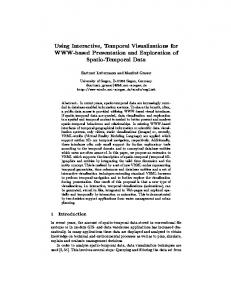
can, e.g., select a particular type of vegetation or a range of vegetation ages. In addition, Tardis supports interactive orthogonal cutting, but in contrast with our previous examples, cutting is always used in combination with 3D rendering. Users can define and manipulate multiple orthogonal cutting planes (Figure 28(a)). Further operations include opening the cube like a book (interactive (volume extraction + rotation)*) or apply a 3D fisheye effect (interactive (volume extraction + translation)*). This fisheye effect, called “Visual Access Distortion”, pushes away voxels from the cursor (Figure 28(b)). 4.4. VISUAL-TimePAcTS

(a) 3D rendering

(b) Space flattening (on top)

Figure 27: Illustration after GeoTime [geo] GeoTime is a carefully-designed commercial system for analyzing spatio-temporal data [geo, KW04]. Events are shown as spheres on a 3D rendering view that can be freely rotated (Figure 27(a)). This view also uses a reference plane, and a semantic volume interpolation operation is applied to indicate event ordering. Users can perform time chopping operations by dragging on a timeline widget. GeoTime also supports time flattening and space flattening. Figure 27(a) shows a space flattening view where time runs from top to bottom, and a reference plane is provided that can be rotated. Thin gray lines connect the two views. Finally, pan & zoom is supported through space chopping + space scaling.

(a)

(b)

(d) Shearing explained

4.3. Tardis

(c)

(e) The result of shearing

Figure 29: VISUAL TimePAcTS [VFC10]. (a) Space Flattening on activities, (b) Oblique flattening, (c) Space flattening on individuals. VISUAL-TimePAcTS is a system for analyzing activity diaries [VFC10]. It uses non-geographical space-time cubes. The cube’s two data axes can be mapped to data dimensions such as individuals, locations, or activities. We focus on the case where one axis maps to individuals while the other axis maps to activities. Activities are also encoded using color.

(a) 3D rendering with multiple (b) 3D rendering with multiple time and space cutting volume extraction+translation

Figure 28: Tardis [CCT∗ 99] and visual access [CFC∗ 96] Tardis [CCT∗ 99, CFC∗ 96] is a system for visualizing environmental data using 3D rendering in combination with advanced space-time cube operations. The voxels in the cube are color-coded depending on the type of vegetation, its age, soil characteristics or the presence of bush fires (Figure 28). Tardis implements interactive semantic filtering: users

VISUAL-TimePAcTS supports linear space flattening on both data axes. Figure 29(a) shows 6 individuals (horizontal axis) and their activities (colors) across time (vertical axis). Figure 29(c) shows the evolution of activities aggregated across all people over time. VISUAL-TimePAcTS supports a seamless transition between the two operations through interactive 3D rendering (Figure 29(c)). Since 3D rendering employs orthographic projection and no shading, it is essentially an oblique flattening operation. VISUAL-TimePAcTS supports a more elaborate spacetime cube operation that prevents visual marks from overlapping due to flattening. In Figure 29(c), for example, individuals are horizontally offset when several of them do the same submitted to Eurographics Conference on Visualization (EuroVis) (2014)


13

activity at the same time. This technique is called shearing by the authors, and is further explained in Figures 29(d), 29(e). This technique is essentially a (linear space cutting + space offset)* + space flattening operation, and is a hybrid between space juxtaposing and space flattening. 4.5. Cubix

(a)

(b)

Figure 31: (a) Video Cubism [FLM00]; (b) V 3 [DC03]. with an interactive volume extraction operation that is defined by manipulating a planar cutting plane (Figure 31(a)). Similary, Khronos projector [CI05] supports manipulation of a non-planar cutting plane using touch or mid-air gestures (Figure 4). V 3 [DC03] (Volume Visualization for Videos) supports different operations, including time juxtaposing and a 3D rendering view that can be combined with a bending operation (Figure 31(b)). V 3 also supports filtering operations that allow removal of pixels of a certain color, or pixels that do not change across a given time period.

Figure 30: Different operations applied to a time-evolving adjacency matrix in Cubix [BPF14b] Cubix is a system for analyzing dynamic weighted networks through adjacency matrix representations [BPF14b]. A 3D rendering provides an overview of the data (Figure 30(a)). Time goes from left to right. Each cell of the cube represents a connection between two nodes at a given time, with size depending on connection weight. Cells can be color-coded according to time, weight, or direction. Cubix supports a range of space-time cube operations, including time juxtaposing (Figure 30(b)), space juxtaposing (detail in Figure 30(d)), animated time cutting , animated space cutting, time flattening and space flattening. For flattening operations, cells can be made translucent to visually aggregate the history of connections. Cubix also supports semantic filtering on connections based on their weight.

Besides the space-time cube systems reviewed in this section, there is a wealth of general 3D visualization systems. Commercial and research tools exist in domains such as geovisualization (e.g., Voxler [Vox], ArcGIS [arc]), scientific visualization (e.g., VTK [SAH00], Matlab [mat] and R [r]), and medical visualization [MTB03]. Although these tools do not treat time as a specific dimension, they can be used to inspire the design of interactive space-time cube systems. 5. General Discussion We now discuss the limitations of our descriptive framework and consider areas for future research, including: unifying our framework with the infovis pipeline model, extending it to other dimensionalities, considering non-planar media such as physical visualizations, characterizing the inner structure of time space cubes, and considering the strengths and weaknesses of different space-time cube operations. 5.1. Comparison with the Infovis Pipeline Model

4.6. Video Cube Systems

Since our framework builds on the notion of composition of operations, it shares similarities with another common model: the infovis reference model, also called the infovis pipeline [CMS99, Chi00, JD13]. The infovis pipeline sees visualization as a data-flow process, i.e., a sequence of stages and transformations that turn raw data into a final image. These transformations commonly include data transformation, visual mapping, presentation mapping and rendering [JD13]. Interactivity is implemented by having data analysts alter these transformations at different stages.

Several space-time cube systems have been proposed to support video analysis [MB98,FLM00,DC03,CI05]. Video Cubism [FLM00] uses a 3D rendering representation together

There is clearly an analogy between transformations and operations. However, the infovis pipeline and our framework differ in several important respects. The infovis pipeline is a

Cubix provides a control widget in the form of a stylized cube, and whose different parts can be clicked or dragged to switch between operations. All operation switches are explained using animated transitions through rotations of the 3D rendering representation, or through staged animations of extraction and rigid transformation operations.


14


general model for visualizations, where the sequence of operations is fixed, but the operations themselves are rather abstract. For example, the pipeline model provides no specific details about what happens in the visual mapping transformation. In contrast, our model only captures a specific family of visualizations (temporal visualizations), its sequence of operations is not fixed, and the operations are more concrete. The infovis pipeline is more general but too high-level to capture the similarities and differences between the visualizations we presented. On the other hand, our model is incomplete in that it does not define how the space-time cube is built. The two models are therefore complementary. Since the infovis pipeline has inspired the software architecture of several infovis tools [Fek04], it is worth considering to what extent the two models can be unified. Several space-time cube operations could in principle be implemented at different stages of the infovis pipeline. For example, time flattening can be performed at the data transformation stage, by aggregating raw data over time. Alternatively, time flattening could be emulated by explicitly rendering a 3D space-time cube on the screen and using a proper camera placement and projection transformation. In that case, it would be implemented at the rendering level. However, these approaches would only provide a very partial support for space-time cube operations. For a full support, our space-time cube needs to be reified as a first-class object. Since it is both abstract and visual, our space-time cube best aligns with the abstract visual form stage of the pipeline [JD13]. Thus space-time cube operations are best seen as presentation mapping transformations, i.e., transformations that turn the abstract visual form into a fullyspecified 2D image or 3D model [JD13]. In other terms, our space-time cube operations can be used to decompose and refine the presentation mapping transformation of the infovis pipeline. We believe that implementing our framework in this way could dramatically facilitate the exploration of a wide range of temporal visualization techniques.

5.2. Other Dimensionalities This review focused on temporal visualizations that involve two spatial dimensions plus time. These two dimensions can be inherently spatial or can result from 2D spatial encodings of abstract data. However, temporal visualizations with other dimensionalities are possible. Most notably, a rich variety of temporal visualizations exist that involve a single spatial dimension plus time, e.g., timelines and time-series visualizations [AMST11]. In principle, our framework still applies if the 3D space-time cube is turned into a 2D space-time plane. Operations analogous to our geometry transformation operations would capture techniques such as spiral visualizations, calendar visualizations or cycle plots [AMST11]. However, since a 2D spacetime plane already naturally maps to a 2D planar display, and

Figure 32: Two physical implementations of the Matrix Cube visualization [BPF14b] for dynamic networks, made by this article’s first author. since the richness of time-series visualizations and timelines mostly stem from the visual encodings used, the usefulness of our framework would be less clear in this case. Other temporal visualization techniques, although less common, show three spatial dimensions plus time. We believe most of them can be captured with operations on 4dimensional space-time hypercubes. For example, Tufte explains how small multiples can be used to show the evolution of a three-dimensional storm [BB95]. This approach amounts to applying a time juxtaposition operation on a space-time hypercube, where each time cutting operation yields a 3D image. Similarly, FromDady [HTC09] uses 3D trails to show the trajectories of airplanes in space. This technique amounts to performing a time flattening on a spacetime hypercube. Extending our framework to higher data dimensionalities is an exciting topic for future research. However, it is less easy to imagine a hypercube than a cube, so the merits of such a conceptual model still remain to be seen. 5.3. Non-Planar Media Throughout this review we assumed the presentation medium to be planar. Although these are by far the most common, other display shapes are being explored in HCI, some of which are even deformable [RPPH12, HV08]. In these cases, the conditions for an operation to be complete are not the same. This opens up a wide range of possibilities for new visualization designs. For example, one implementation of the Khronos projector (Figure 4) employs back projection on a freely deformable cloth, allowing the use of non-planar cutting operations that are complete. In addition, physical visualizations make it possible to faithfully display 3D space-time cubes without any additional operations [JDF13, JD13]. Many such visualizations have been already crafted by scientists, artists and designers [DJ13]. Physical temporal visualizations can even be made modular to support interactive space-time cube operations. Figure 32 shows two physical representations of a dynamic netsubmitted to Eurographics Conference on Visualization (EuroVis) (2014)


15

work [BPF14b] made of laser-cut and laser-engraved acrylic. The left version supports interactive time cutting while the right version supports interactive space cutting. Cuts can be taken apart and manipulated freely, allowing for time juxtaposing and space juxtaposing as well as time flattening and space flattening, if viewed from a proper orthogonal angle and distance. For another example see [STB].

5.4. The Inner Structure of Space-Time Cubes In this review we considered space-time cubes as monolithic entities. Two space-time cubes can however look quite different, depending on what data is visualized: migration of animals, earthquakes, changes in vegetation and ecosystems, networks with changing connections, surveillance videos, or scatterplots evolving over time. We can refer to this lowerlevel decomposition as the cube’s inner structure. Inner structure is likely to be an important factor when choosing between space-time cube operations. For example, videos produce maximally dense inner structures and therefore are not well-suited to 3D rendering, unless complementary operations such as filtering are used (Figure 31(b)). Structures that present large variations over time may not be well-suited to time juxtaposing because objects could be difficult to relate across time slices. We plan to extend our descriptive framework by characterizing different types of inner structures for space-time cubes.

5.5. Which Operation to Choose? Again, our contribution is a descriptive conceptual framework, and we chose not consider the relative merits and limitations of different techniques. We believe that a detailed descriptive model is a necessary first step, before considering performance issues. The question however remains as of which operation works best under which context. Several studies comparing space-time cube operations have been reported in the past. Many of them compared animation (usually animated time cutting) against static visualizations (usually time juxtaposing) [TMB02, GMH∗ 06, RFF∗ 08, APP11, FQ11, AP12b], finding benefits and drawbacks for both approaches. Other studies evaluated space time-cube representations (i.e., 3D rendering) against a range of baseline conditions, including time flattening [KDA∗ 09, WvdWvW09, KK12, AABW12], time cutting [WvdWvW09, BCH07], and space cutting [AABW12]. Although such empirical investigations are crucial for the advancement of science, only a subset of all possible operations have been covered, and many of the existing findings are hard to generalize beyond the domain, type of data, and operation parameters used in the stimuli. For example, animation can mean either animated time cutting or interactive time cutting, and space-time cube visualizations can be implemented in a multitude of ways, including in the content submitted to Eurographics Conference on Visualization (EuroVis) (2014)

Figure 33: Visualization of energy consumption over time [vWvS99]. One horizontal axis is mapped to days while the other one is mapped to hours. transformations they use (e.g., aggregation [BCH07] or filtering [AABW12]), and in the interactions they implement. Overall, findings are very hard to compare for a lack of a consistent descriptive terminology. A clear and descriptive framework would allow us to better structure this body of evidence and tease apart the effects of different subtle design features and to better control for confounds. We showed how many temporal visualization techniques can be decomposed into elementary operations. These operations can be combined in many ways or made dynamic at different levels (either through animation or interaction). The characterization of the inner structure of space-time cubes, may already provide many elements to discuss the practical strengths and weaknesses of space-time cube operations, mostly based on well-established knowledge on perception and HCI, and on common sense. Running studies for answering specific research questions will naturally remain important, and we hope our descriptive framework will facilitate the design of such studies and the discussion of findings in a more informative manner. 5.6. Other Limitations Our framework is designed as a thinking tool. Like any model, it is necessarily incomplete. First, our taxonomy of elementary operations in Figure 24 is not meant to cover all possible operations. Second, our framework does not provide much guidance for interaction design: the design space for interactive operations has only been partially explored. Finally, not all techniques for visualizing temporal data can be captured with space-time cubes. For example, temporal data can be visualized using two time axes instead of a single data axis (see Figure 33). Our framework is not meant to restrict creativity but rather to help visualization designers find new solutions, extend or generalize existing ones, and think out of the box.

16


Again, our framework assumes that the space-time cube already exists. It does not provide guidance for producing the space-time cube itself. For abstract data, many visual mappings can be used to produce individual slices. For example, locations on a map can yield values for altitude, temperature, rain, vegetation and soil type. How to visualize all these attributes at any particular point in time is a general problem of information visualization, but the choice may also affect the efficiency of later space-time cube operations.

6. Conclusion

References [AA99] A NDRIENKO G., A NDRIENKO N.: Making a GIS intelligent: CommonGIS project view. Proceedings of AGILE99 (1999), 19–24. 11 [AA03] A NDRIENKO N., A NDRIENKO G.: Visual Data Exploration using Space-Time Cube. In Proceedings of International Cartographic Conference (Durban, South Africa, 2003), International Cartographic Association, pp. 1981–1983. 2 [AA04a] A NDRIENKO G., A NDRIENKO N.: Research on visual analysis of spatio-temporal data at Fraunhofer AIS: an overview of history and functionality of CommonGIS. http://geoanalytics.net/and/ 2004. KDworkshopPaper2004/KDworkshop.html, [online, accessed:12-apr-2014]. 11

We reviewed various techniques to visualize temporal data, by describing them as sequences of parametric operations applied to a conceptual space-time cube. Our operations are independent from the underlying data and can be applied across a range of application domains, be they cartography, dynamic network analysis, geopolitics, or video analytics.

[AA04b] A NDRIENKO N., A NDRIENKO G.: Interactive visual tools to explore spatio-temporal variation. In Proceedings of the working conference on Advanced visual interfaces (New York, NY, USA, 2004), AVI ’04, ACM, pp. 417–420. 1, 2, 6

By introducing domain-agnostic concepts and a clear terminology, this article aims at facilitating the comparison of different approaches for visualizing temporal data. Existing visualizations from one data domain can be analyzed in terms of elementary operations and then be adapted to other domains and problems.

[AAB∗ 11] A NDRIENKO G., A NDRIENKO N., BAK P., K EIM D., K ISILEVICH S., W ROBEL S.: A Conceptual Framework and Taxonomy of Techniques for Analyzing Movement. Journal of Visual Languages and Computing 22, 3 (June 2011), 213–232. 1

By giving a better vision of the richness of the design space, we hope our model will also motivate the exploration of new approaches. It also stresses the importance of developing fully-integrated interactive systems and toolkits that can support a range of techniques in a consistent manner.

[AAH11] A NDRIENKO G., A NDRIENKO N., H EURICH M.: An Event-based Conceptual Model for Context-aware Movement Analysis. International Journal on Geographic Information Science 25, 9 (Sept. 2011), 1347–1370. 1

Our model also aims at facilitating the design of studies and discussing their results in a more informative manner. We hope the presented terminology and low-level concepts will help design better experiments that tease out important factors in dynamic data visualization. Many more controlled studies are needed to understand the trade-offs between different space-time cube operations and how they perform depending on the task, the data, and the people that use them. This work mostly arose out of the need to teach temporal information visualization to undergrad students. We therefore hope that it will help other people teach this field effectively, by providing a clear structure and a clear terminology on which to base higher-level discussions and analyses.

Acknowledgements Collaboration on this work was initiated by Dagstuhl Seminar “Putting Data on the Map 12261”, June 2012, and supported in part by NSERC, SMART Technologies, AITF, Surfnet and GRAND NCE, as well as by Clique Strategic Research Cluster funded by Science Foundation Ireland (SFI) Grant No. 08/SRC/I1407.

[AA12] A NDRIENKO N., A NDRIENKO G.: Visual analytics of movement: An overview of methods, tools and procedures. Information Visualization 12, 1 (2012), 3–24. 1

[AABW12] A NDRIENKO G., A NDRIENKO N., B URCH M., W EISKOPF D.: Visual analytics methodology for eye movement studies. Visualization and Computer Graphics, IEEE Transactions on 18, 12 (Dec 2012), 2889–2898. 15

[AMM∗ 07] A IGNER W., M IKSCH S., M ÜLLER W., S CHU MANN H., T OMINSKI C.: Visualizing Time-oriented data-A Systematic View. Computers and Graphics 31, 3 (June 2007), 401–409. 1 [AMST11] A IGNER W., M IKSCH S., S CHUMANN H., T OMIN SKI C.: Visualization of Time-Oriented Data, 1st ed. HumanComputer Interaction. Springer Verlag, 2011. 1, 14 [AP12a] A RCHAMBAULT D., P URCHASE H. C.: Mental Map Preservation Helps User Orientation in Dynamic Graphs. In Proceedings of Graph Drawing (2012), GD ’12, Springer, pp. 475– 486. 10 [AP12b] A RCHAMBAULT D., P URCHASE H. C.: The Mental Map and Memorability in Dynamic Graphs. In Proceedings of Pacific Visualization Symposium (2012), PacificVis ’12, IEEE Computer Society, pp. 89–96. 15 [APP11] A RCHAMBAULT D., P URCHASE H., P INAUD B.: Animation, Small Multiples, and the Effect of Mental Map Preservation in Dynamic Graphs. IEEE Transactions on Visualization and Computer Graphics 17, 4 (2011), 539–552. 15 [arc] ArcGIS. http://www.esri.com/software/ arcgis. [online, accessed:02-apr-2014]. 13 [AS] A RIS A., S HNEIDERMAN B.: NVSS: Network Visualization by Semantic Substrates. http://www.cs.umd.edu/ hcil/nvss/. [online, accessed:02-apr-2014]. 6 [ATMS∗ 11] A HN J.-W., TAIEB -M AIMON M., S OPAN A., P LAISANT C., S HNEIDERMAN B.: Temporal visualization of social network dynamics: prototypes for nation of neighbors. In Proceedings of International conference on Social computing, submitted to Eurographics Conference on Visualization (EuroVis) (2014)

B. Bach & P. Dragicevic / A Review of Temporal Data VisualizationsBased on Space-Time Cube Operations behavioral-cultural modeling and prediction (Berlin, Heidelberg, 2011), SBP’11, Springer-Verlag, pp. 309–316. 11 [BB95] BAKER M. P., B USHELL C.: After the storm: Considerations for information visualization. Computer Graphics and Applications, IEEE 15, 3 (1995), 12–15. 14 [BBL12] B OYANDIN I., B ERTINI E., L ALANNE D.: A Qualitative Study on the Exploration of Temporal Changes in Flow Maps with Animation and Small-Multiples. Computer Graphics Forum 31, 3pt2 (2012), 1005–1014. 5 [BC03] B RANDES U., C ORMAN S. R.: Visual unrolling of network evolution and the analysis of dynamic discourse. Information Visualization 2, 1 (Mar. 2003), 40–50. 7 [BCD∗ 12] B ORGO R., C HEN M., DAUBNEY B., G RUNDY E., H EIDEMANN G., H ÖFERLIN B., H ÖFERLIN M., L EITTE H., W EISKOPF D., X IE X.: State of the Art Report on Video-Based Graphics and Video Visualization. Computer Graphics Forum 31, 8 (Dec. 2012), 2450–2477. 1 [BCH07] B RUNSDON C., C ORCORAN J., H IGGS G.: Visualising space and time in crime patterns: A comparison of methods. Computers, Environment and Urban Systems 31, 1 (2007), 52 – 75. Extracting Information from Spatial Datasets. 15

17

WAMPLER K.: A system for graph-based visualization of the evolution of software. In Proceedings of ACM Symposium on Software Visualization (New York, NY, USA, 2003), SoftVis ’03, ACM, pp. 77–ff. 4, 5 [CLK00] C HOI B.-T., L EE S.-H., KO S.-J.: New frame rate upconversion using bi-directional motion estimation. IEEE Transactions on Consumer Electronics 46, 3 (2000), 603–609. 9 [CMS99] C ARD S. K., M ACKINLAY J. D., S HNEIDERMAN B. (Eds.): Readings in Information Visualization: Using Vision to Think. Morgan Kaufmann Publishers Inc., San Francisco, CA, USA, 1999. 13 [DC03] DANIEL G., C HEN M.: Video Visualization. In Proceedings of IEEE Visualization (Washington, DC, USA, 2003), VIS ’03, IEEE Computer Society, pp. 409–416. 9, 10, 13 [DE02] DWYER T., E ADES P.: Visualising a Fund Manager Flow Graph with Columns and Worms. In Proceedings of International Conference on Information Visualisation (2002), IV ’02, pp. 147–152. 7 [DG04] DWYER T., G ALLAGHER D. R.: Visualising changes in fund manager holdings in two and a half-dimensions. Information Visualization 3, 4 (Dec. 2004), 227–244. 7

[BDH04] BARTOLI A., DALAL N., H ORAUD R.: Motion Panoramas. Computer Animation and Virtual Worlds, 15 (2004), 501–517. 4

[DJ13] D RAGICEVIC P., JANSEN Y.: List of Physical Visualizations. http://www.tinyurl.com/physvis, 2013. [Online; accessed 04-Sep-2013]. 14

[BGPS07] BATTIATO S., G ALLO G., P UGLISI G., S CELLATO S.: SIFT features tracking for video stabilization. In Proceedings of Conference on Image Analysis and Processing (2007), ICIAP ’07, IEEE, pp. 825–830. 10

[DV10] D EMŠAR U., V IRRANTAUS K.: Space–time density of trajectories: exploring spatio-temporal patterns in movement data. International Journal of Geographical Information Science 24, 10 (2010), 1527–1542. 10

[BN11] B RANDES U., N ICK B.: Asymmetric Relations in Longitudinal Social Networks. IEEE Transactions on Visualization and Computer Graphics 17, 12 (Dec. 2011), 2283–2290. 6 [BPF14a] BACH B., P IETRIGA E., F EKETE J.-D.: GraphDiaries: Animated Transitions and Temporal Navigation for Dynamic Networks. IEEE Transactions on Visualization and Computer Graphics (2014). to appear. 5, 10, 11 [BPF14b] BACH B., P IETRIGA E., F EKETE J.-D.: Visualizing Dynamic Networks with Matrix Cubes. In Proceedings of SIGCHI Conference on Human Factors and Computing Systems (New York, NY, USA, 2014), CHI ’14, ACM. to appear. 9, 10, 11, 13, 14, 15 [BVB∗ 11]

B URCH M., V EHLOW C., B ECK F., D IEHL S., W EISKOPF D.: Parallel Edge Splatting for Scalable Dynamic Graph Visualization. Visualization and Computer Graphics, IEEE Transactions on 17, 12 (2011), 2344–2353. 6

[CCT∗ 99] C ARPENDALE S. T., C OWPERTHWAITE D. J., T IGGES M., FALL A., F RACCHIA F. D.: The Tardis: A Visual Exploration Environment for Landscape Dynamics. In Proceedings of Conference on Visual Data Exploration and Analysis (1999), no. 3643, pp. 110–119. 2, 9, 10, 12 [CFC∗ 96] C ARPENDALE S. T., FALL A., C OWPERTHWAITE D. J., FALL J., F RACCHIA F. D.: Case study: visual access for landscape event based temporal data. In Proceedings of Visualization (1996), VIS ’06, IEEE Computer Society, pp. 425–428. 12 [Chi00] C HI E. H.- H .: A Taxonomy of Visualization Techniques using the Data State Reference Model. In Proceedings of IEEE Symposium on Information Visualization (2000), Infovis ’00, IEEE, pp. 69–75. 13 [CI05] C ASSINELLI A., I SHIKAWA M.: Khronos Projector. In Proceedings of SIGGRAPH 2005 (2005). 2, 13 [CKN∗ 03]

C OLLBERG C., KOBOUROV S., NAGRA J., P ITTS J.,


[FBS06] FALKOWSKI T., BARTELHEIMER B., S PILIOPOULOU M.: Mining and Visualizing the Evolution of Subgroups in Social Networks. In Web Intelligence, 2006. WI 2006. IEEE/WIC/ACM International Conference on (2006), pp. 52–58. 6 [Fek04] F EKETE J.: The infovis toolkit. In Information Visualization, 2004. INFOVIS 2004. IEEE Symposium on (2004), IEEE, pp. 167–174. 14 [FLM00] F ELS S., L EE E., M ASE K.: Techniques for Interactive Video Cubism (poster session). In Proceedings of International conference on Multimedia (New York, NY, USA, 2000), MULTIMEDIA ’00, ACM, pp. 368–370. 2, 9, 13 [FQ11] FARRUGIA M., Q UIGLEY A.: Effective temporal graph layout: A comporative stydy of animations versus statuc display methods. Information Visualization (2011), 47–64. 15 [GAA04] G ATALSKY P., A NDRIENKO N., A NDRIENKO G.: Interactive Analysis of Event Data Using Space-Time Cube. In Proceedings of the Information Visualisation, Eighth International Conference (Washington, DC, USA, 2004), IV ’04, IEEE Computer Society, pp. 145–152. 7 [geo] GeoTime. http://www.geotime.com. [Online; accessed 24-Jan-2014]. 12 [GHW09] G ROH G., H ANSTEIN H., W OERNDL W.: Interactively Visualizing Dynamic Social Networks with DySoN. In Workshop on Visual Interfaces to the Social and the Semantic Web (February 2009). 7 [GMH∗ 06] G RIFFEN A. L., M AC E ACHREN A. M., H ARDISTY F., S TEINER E., L I B.: A Comparison of Animated Maps with Static Small-Multiple Maps for Visually Identifying Space-Time Clusters. Annals of the Association of American Geographers 96, 4 (2006), 740–753. 15 [Gre11] G RETCHEN P.: A Cartographer’s Toolkit - Small Multiples. http://www.gretchenpeterson.com/blog/ small-multiples, 2011. [Online; accessed 24-Jan-2014]. 5

18


[Har99] H ARRIS R. L.: Information Graphics: A Comprehensive Illustrated Reference. Oxford University Press, New York, 1999. 1 [HEF∗ 13] H URTER C., E RSOY O., FABRIKANT S., K LEIN T., T ELEA A.: Bundled Visualization of Dynamic Graph and Trail Data. IEEE Transactions on Visualization and Computer Graphics, 99 (2013). 10, 11 [HET12] H URTER C., E RSOY O., T ELEA A.: Graph Bundling by Kernel Density Estimation. Computer Graphics Forum 31 (June 2012), 865–874. 11 [HSCW13] H ADLAK S., S CHUMANN H., C AP C. H., W OLLEN BERG T.: Supporting the Visual Analysis of Dynamic Networks by Clustering associated Temporal Attributes. IEEE Transactions on Visualization and Computer Graphics 19, 12 (2013), 2267– 2276. 6 [HTC09] H URTER C., T ISSOIRES B., C ONVERSY S.: FromDaDy: Spreading Aircraft Trajectories Across Views to Support Iterative Queries. IEEE Transactions on Visualization and Computer Graphics 15, 6 (2009), 1017–1024. 14 [HV08] H OLMAN D., V ERTEGAAL R.: Organic user interfaces: designing computers in any way, shape, or form. Communications of the ACM 51, 6 (2008), 48–55. 14 [Hä70] H ÄGERSTRAND T.: What about People in Regional Science. In Papers of the Regional Science Association (1970). 2 [JD13] JANSEN Y., D RAGICEVIC P.: An interaction Model for Visualizations Beyond The Desktop. IEEE Transactions on Visualization and Computer Graphics (2013). In press. 7, 13, 14 [JDF13] JANSEN Y., D RAGICEVIC P., F EKETE J.-D.: Evaluating the Efficiency of Physical Visualizations. In Proceedings of the SIGCHI Conference on Human Factors in Computing Systems (2013), CHI ’13, ACM, pp. 2593–2602. 14 [KDA∗ 09] K RISTENSSON P., DAHLBACK N., A NUNDI D., B JORNSTAD M., G ILLBERG H., H ARALDSSON J., M ARTENS SON I., N ORDVALL M., S TAHL J.: An Evaluation of Space Time Cube Representation of Spatiotemporal Patterns. IEEE Transactions on Visualization and Computer Graphics 15, 4 (July 2009), 696–702. 15 [KK12] K VELADZE I., K RAAK M.-J.: What do we know about the space-time cube from cartographic and usability perspective? In Proceedings of the 2012 AutoCarto International Symposium on Automated Cartography (2012), AuroCarto’12. 15 [Kra03] K RAAK M. J.: The Space-Time Cube revisited from a Geovisualization Perspective. Proceedings of the 21st International Cartographic Conference (2003), 1988–1996. 2, 7 [KW04] K APLER T., W RIGHT W.: GeoTime Information Visualization. In Proceedings of IEEE Information Visualization (Washington, DC, USA, 2004), INFOVIS ’04, IEEE Computer Society, pp. 25–32. 9, 12 [LNS11] L IU Z., NAVATHE S., S TASKO J.: Network-based visual analysis of tabular data. In Proceedings of Conference on Visual Analytics Science and Technology (2011), VAST ’11, pp. 41–50. 5 [Mar78] M AREY É.-J.: La méthode graphique dans les sciences expérimentales et particulièrement en physiologie et en médecine. G. Masson, 1878. 4, 5

[McC94] M C C LOUD S.: Understanding Comics. HarperCollins, 1994. 5 [MTB03] M C G UFFIN M. J., TANCAU L., BALAKRISHNAN R.: Using Deformations for Browsing Volumetric Data. In Proceedings of IEEE Visualization (October 2003), VSI ’03, pp. 401– 408. 13 [Mun08] M UNZNER T.: Process and Pitfalls in Writing Information Visualization Research Papers. In Information Visualization. Springer-Verlag, 2008, p. 134–153. 3 [Muy87] M UYBRIDGE E.: Animal Locomotion. Published under the auspices of the University of Pennsylvania, 1887. 5 [PJH05] P ETROVIC N., J OJIC N., H UANG T. S.: Adaptive Video Fast Forward. Multimedia Tools and Applications 26, 3 (2005), 327–344. 10 [r]

R. http://www.r-project.org/. accessed:02-apr-2014]. 13

[online,

[RFF∗ 08] ROBERTSON G., F ERNANDEZ R., F ISHER D., L EE B., S TASKO J.: Effectiveness of Animation in Trend Visualization. IEEE Transactions on Visualization and Computer Graphics 14, 6 (Nov. 2008), 1325–1332. 9, 10, 11, 15 [RM13] RUFIANGE S., M C G UFFIN M. J.: DiffAni: Visualizing Dynamic Graphs with a Hybrid of Difference Maps and Animation. IEEE Transactions on Visualization and Computer Graphics 19, 12 (2013), 2556–2565. 5, 10, 11 [Ros06] ROSLING H.: Stats that reshape your worldview. http://www.ted.com/talks/hans_rosling_ the_good_news_of_the_decade.html, 2006. [online, accessed:24-jan-2014]. 3, 10, 11 [RPPH12] R ASMUSSEN M. K., P EDERSEN E. W., P ETERSEN M. G., H ORNBÆK K.: Shape-changing interfaces: a review of the design space and open research questions. In Proceedings of the SIGCHI Conference on Human Factors in Computing Systems (2012), ACM, pp. 735–744. 14 [SA06] S HNEIDERMAN B., A RIS A.: Network Visualization by Semantic Substrates. IEEE Transactions on Visualization and Computer Graphics 12, 5 (2006), 733–740. 6 [SAH00] S CHROEDER W. J., AVILA L. S., H OFFMAN W.: Visualizing with VTK: a tutorial. Computer Graphics and Applications, IEEE 20, 5 (2000), 20–27. 13 [SRdJ05] S HANBHAG P., R HEINGANS P., DES JARDINS M.: Temporal Visualization of Planning Polygons for Efficient Partitioning of Geo-Spatial Data. In Proceedings of the 2005 IEEE Symposium on Information Visualization (Washington, DC, USA, 2005), INFOVIS ’05, IEEE Computer Society, pp. 28–. 1, 2, 6 [STB] S TUSAK S., TABARD A., B UTZ A.: Can physical visualizations support analytical tasks? In Poster Abstracts of IEEE VIS 2013. 15 [TBC13] T HUDT A., BAUR D., C ARPENDALE S.: Visits: A Spatiotemporal Visualization of Location Histories. [online, accessed:24-jan-2014]. 5, 11 [TGF08] TANG A., G REENBERG S., F ELS S.: Exploring Video Streams using Slit-Tear Visualizations. In Proceedings of the working conference on Advanced visual interfaces (New York, NY, USA, 2008), AVI ’08, ACM, pp. 191–198. 5, 6

[mat] MatLab. http://www.mathworks.fr/products/ matlab/. [online, accessed:02-apr-2014]. 13

[TMB02] T VERSKY B., M ORRISON J., B ETRANCOURT M.: Animation: Can it facilitate? International Journal of HumanComputer Studies 57, 4 (2002), 247–262. 15

[MB98] M ACKAY W., B EAUDOUIN -L AFON M.: DIVA: Exploratory Data Analysis with Multimedia Streams. In Proceedings of SIGCHI Conference on Human Factors in Computing Systems (apr 1998), CHI ’98, ACM, pp. 416–423. 13

[TSAA12] T OMINSKI C., S CHUMANN H., A NDRIENKO G., A NDRIENKO N.: Stacking-Based Visualization of Trajectory Attribute Data. Visualization and Computer Graphics, IEEE Transactions on 18, 12 (Dec 2012), 2565–2574. 9 submitted to Eurographics Conference on Visualization (EuroVis) (2014)

B. Bach & P. Dragicevic / A Review of Temporal Data VisualizationsBased on Space-Time Cube Operations [Tuf] T UFTE E.: Megan Jaegerman’s brilliant news graphhttp://www.edwardtufte.com/bboard/ ics. [online, q-and-a-fetch-msg?msg_id=0002w4. accessed:12-apr-2014]. 4 [Tuf86] T UFTE E. R.: The visual display of quantitative information. Graphics Press, Cheshire, CT, USA, 1986. 1, 3, 4, 5 [TV07] T RUONG B. T., V ENKATESH S.: Video Abstraction: A systematic Review and Classification. ACM Transactions on Multimedia Computing, Communications, and Applications (TOMCCAP) 3, 1 (2007), 3. 5 [VFC10] V ROTSOU K., F ORSELL C., C OOPER M.: 2D and 3D representations for feature recognition in time geographical diary data. Information Visualization 9, 4 (Dec. 2010), 263–276. 12 [Vox] Voxler. http://www.goldensoftware.com/ products/voxler. [online, accessed:02-apr-2014]. 13 [VWD04] V IÉGAS F. B., WATTENBERG M., DAVE K.: Studying cooperation and conflict between authors with history flow visualizations. In Proceedings of the SIGCHI Conference on Human Factors in Computing Systems (New York, NY, USA, 2004), CHI ’04, ACM, pp. 575–582. 6, 10 [vWvS99] VAN W IJK J. J., VAN S ELOW E. R.: Cluster and Calendar Based Visualization of Time Series Data. In Proceedings of the IEEE Symposium on Information Visualization (Washington, DC, USA, 1999), INFOVIS ’99, IEEE Computer Society, pp. 4–. 15 [Wik13] W IKIMEDIA: "stroke order project". http://www. tinyurl.com/strokeOrderProject, 2013. [Online; accessed 24-Jan-2014]. 4, 5 [WvdWvW09] W ILLEMS N., VAN DE W ETERING H., VAN W IJK J. J.: Visualization of Vessel Movements. In Proceedings of the 11th Eurographics / IEEE- VGTC Conference on Visualization (Aire-la-Ville, Switzerland, 2009), EuroVis’09, Eurographics Association, pp. 959–966. 15

Biography Benjamin Bach is a PhD student in the Aviz group at INRIA, France, since 2011. He received his Masters Degree in 2010 from the Department of Computer Science at the University of Technology, Dresden, Germany. His research focuses on network visualization, visualization of temporal data, interaction for information visualization. Pierre Dragicevic is a permanent researcher in the Aviz group at INRIA, France, since 2007. He is doing research on human-computer interaction and information visualization, with a focus on animation, direct manipulation, physical visualization, visual perception and decision making. Daniel Archambault is a lecturer at Swansea University (since 2013). His research interests include information visualization, graph drawing, and perceptual issues in visualization. Daniel has worked in the area of dynamic graph drawing and has conducted human-centered experiments involving presentation methods for dynamic graphs such as animation and small multiples as well as drawing stability (or the “mental map”). Christophe Hurter is an associate professor at the Interactive computing laboratory (LII) at the French Civil Aviation University (ENAC) in Toulouse, France, since 2011. submitted to Eurographics Conference on Visualization (EuroVis) (2014)

19

His research interests lie in the areas of information visualization and human-computer interaction, with a focus on visualization of multivariate data in space and time, the design of scalable visual interfaces and the development of pixelbased algorithms such as bundling rendering techniques. Sheelagh Carpendale is a professor at University of Calgary, where she also holds a Canada Research Chair in Information Visualization. She leads the Innovations in Visualization (InnoVis) Research Group. Her research on information visualization, large interactive displays, and new media draws on her interdisciplinary background in art, design and computer science. She has contributed a number of novel techniques for temporal data visualization.

A Review of Temporal Data Visualizations Based on ... - HAL-Inria

A Review of Temporal Data Visualizations Based on ... - HAL-Inria

Suggest Documents