A Riemannian Approach to Diffusion Tensor Images ... - CiteSeerX

A Riemannian Approach to Diffusion Tensor Images Segmentation Christophe Lenglet1 , Mika¨el Rousson2 , Rachid Deriche1 , Olivier Faugeras1 , St´ephane Lehericy3 , and Kamil Ugurbil3 1

3

I.N.R.I.A, 2004 route des lucioles, 06902 Sophia-Antipolis, France {clenglet, der, faugeras}@sophia.inria.fr 2 Siemens Corporate Research, 755 College Road East, Princeton, NJ 08540, USA [email protected] CMRR, University of Minnesota, 2021 6th Street SE, Minneapolis, MN 55455, USA {lehericy, kamil}@cmrr.umn.edu

Abstract. We address the problem of the segmentation of cerebral white matter structures from diffusion tensor images. Our approach is grounded on the theoretically well-founded differential geometrical properties of the space of multivariate normal distributions. We introduce a variational formulation, in the level set framework, to estimate the optimal segmentation according to the following hypothesis: Diffusion tensors exhibit a Gaussian distribution in the different partitions. Moreover, we must respect the geometric constraints imposed by the interfaces existing among the cerebral structures and detected by the gradient of the diffusion tensor image. We validate our algorithm on synthetic data and report interesting results on real datasets. We focus on two structures of the white matter with different properties and respectively known as the corpus callosum and the corticospinal tract.

1

Introduction

Diffusion magnetic resonance imaging is a relatively new modality [1] able to quantify the anisotropic diffusion of water molecules in highly structured biological tissues. As of today, it is the only non-invasive method that allows us to distinguish the anatomical structures of the cerebral white matter. Diffusion tensor imaging [2] models the probability density function of the three-dimensional molecular motion, at each voxel of a diffusion MR image, by a normal distribution of 0-mean and whose covariance matrix is given by the diffusion tensor. Numerous algorithms have been proposed to perform a robust estimation of this tensor field (see [3] and references therein). Among other applications, DTI is extremely useful in order to identify the neural connectivity patterns of the human brain [4], [5], [6]. Most of the existing techniques addressing this last issue work on a fiber-wise basis. In other words, they do not take into account the global coherence that exists among fibers of a given tract. Recent work by Corouge et al. [7] has proposed to cluster and align fibers by local shape parameterization so that a statistical analysis of the tract geometrical and physiological properties G.E. Christensen and M. Sonka (Eds.): IPMI 2005, LNCS 3565, pp. 591–602, 2005. c Springer-Verlag Berlin Heidelberg 2005 °

592

C. Lenglet et al.

can be carried out. This work relies on the extraction of a set of streamlines by the method proposed in [4] which is known to be sensible to noise and unreliable in areas of fiber crossings. For these reasons, we propose to directly perform the segmentation of diffusion tensor images in order to extract neural fiber bundles. To our knowledge, the only approaches addressing the issue of white matter internal structures segmentation are [8], [9], [10], [11], [12], [13], [14] and [15] We hereafter draw a quick state of the art of these techniques. Zhukov et al. [8] define an invariant anisotropy measure in order to drive the evolution of a level set and isolate strongly anisotropic regions of the brain. Alternatively, Wiegell et al. [9], Feddern et al. [10], Rousson et al. [11], Wang et al. [12] and [13], Lenglet et al. [14], and Jonasson et al. [15] use or propose different measures of dissimilarity between full diffusion tensors. In [9], [12] and [11], the authors use the Frobenius norm of the difference of tensors. A spatial coherence or a regularity term was used in the first two methods, respectively in a k-means algorithm or an active contour model to perform the segmentation of different cerebral structures such as the thalamus nuclei or the corpus callosum. The third method used a region-based surface propagation. In [12], a generalization of the region-based active contours to matrix-valued images is proposed. It is consequently restricted to the 2D case. In [10], partial differential equations based on mean curvature motion, self-snakes and geodesic active contour models are extended to two-dimensional and three-dimensional tensor-valued images. This method still relies on the Euclidean metric between tensors. The authors apply this framework to the regularization and segmentation of diffusion tensor images. In [15], the authors introduce a geometric measure of dissimilarity by computing the normalized tensor scalar product of two tensors, which can be interpreted as a measure of overlap. Finally, the methods exposed in [13] and [14] rely on the symmetrized Kullback-Leibler divergence to derive an affine invariant dissimilarity measure between diffusion tensors. Contribution: Our main contributions are threefold: First, the major difference with all the existing approaches is the rigorous differential geometrical framework, strongly rooted in the information geometry and used to express a Gaussian law between diffusion tensors. We overcome the classical hypothesis considering covariance matrices as a linear space. Hence, we define relevant statistics to model the distribution of diffusion tensors. We also use a consistent gradient of the tensor field to detect the boundaries of various structures in the white matter. We then propose a variational formulation of the segmentation problem, in the level set framework, to evolve a surface toward the optimal partition of the data. We finally validate our approach on synthetic and real datasets. Organization of the Paper: Section 2 first reviews necessary material related to the Riemannian geometry of the multivariate normal model. It then introduces the numerical schemes used to approximate a Gaussian law for diffusion tensors. We finally describe how to compute the gradient of a tensor field. Section 3 sets up the Bayesian formulation of the segmentation problem that we

A Riemannian Approach to Diffusion Tensor Images Segmentation

593

use throughout this paper. Section 4 presents and discusses experimental results on synthetic and real DTI datasets.

2

Statistics and Geometry of Diffusion Tensors Fields

As in [16], we can consider the family of three-dimensional normal distributions with 0-mean as the 6-dimensional parameter space of variances-covariances M = {θ : θ = (θ1 , ..., θ6 ) ∈ R6 }. This simply translates the fact that, for diffusion MRI, the average displacement of spins in a voxel is zero. We identify M with S + (3, R), the set of 3×3 real symmetric positive-definite matrices, e.g. covariance matrices whose independent components are denoted by θi . Following the work by Rao [17] and Burbea-Rao [18], where a Riemannian metric was introduced in term of the Fisher information matrix, it is possible to define notions such as the geodesic distance, the curvature, the mean, and the covariance matrix. The basis of the tangent space TΣ S + (3, R) = SΣ (3, R) at Σ ∈ S + (3, R) is taken to be as in [19] and denoted by Ei , i = 1, ..., 6. We now detail the geometry of S + (3, R) and propose an original formulation for a generalized Gaussian law on this manifold. Relying on the explicit, and very simple, expression of the squared geodesic distance gradient, we show how to compute the spatial gradient of a diffusion tensor image. 2.1

Differential Geometry of Multivariate Normal Distributions

The fundamental mathematical tools needed to derive our numerical schemes were detailed in [19], [20], [21], [22], [23] and [24]. Without employing the information geometry associated to the Fisher information matrix but instead, identifying S + (3, R) with the quotient space GL+ (3, R)/SO(3, R), other works such as [25] and [26] recently used similar ideas to derive statistical or filtering tools on tensors fields. Metric Tensor, Geodesics and Geodesic Distance: The metric tensor for S + (3, R), derived from the Fisher information matrix is given by the following theorem: Theorem 1. The Riemannian metric for the space S + (3, R) of multivariate normal distributions with zero mean is given, ∀Σ ∈ S + (3, R) by: gij = g(Ei , Ej ) = hEi , Ej iΣ =

1 tr(Σ −1 Ei Σ −1 Ej ) 2

i, j = 1, ..., 6

(1)

In practice, this means that for any tangent vectors A, B, their inner product relative to Σ is hA, BiΣ = 12 tr(Σ −1 AΣ −1 B). We recall that, if Σ : t 7→ Σ(t) ∈ S + (3, R), ∀t ∈ [t1 , t2 ] ⊂ R denotes a curve segment in S + (3, R) between two normal distributions parameterized by Σ1 and ´1/2 R t2 ³P6 dθi (t) dθj (t) dt Σ2 , its length is expressed as: LΣ (Σ1 ,Σ2 ) = t1 i,j=1 gij (Σ(t)) dt dt

As stated for example in [24], the geodesic starting from Σ(t1 ) ∈ S + (3, R) in the

594

C. Lenglet et al.

˙ 1 ) ∈ S(3, R) is given by: direction V = Σ(t Σ(t) = Σ(t1 )1/2 exp (tΣ(t1 )−1/2 V Σ(t1 )−1/2 )Σ(t1 )1/2 ∀t ∈ [t1 , t2 ]

(2)

We recall that the geodesic distance D between any two element Σ1 and Σ2 is the length of the minimizing geodesic between Σ1 and Σ2 : D(Σ1 , Σ2 ) = inf {LΣ (Σ1 , Σ2 ) : Σ1 = Σ(t1 ), Σ2 = Σ(t2 )} Σ

It is given by the following theorem, whose original proof is available in an appendix of [27] but different versions can also be found in [19] and [23]. Theorem 2. (S.T. Jensen, 1976) Consider the family of multivariate normal distributions with common mean vector but different covariance matrices. The geodesic distance between two members of the family with covariance matrices Σ1 and Σ2 is given by v r u m u1 X 2 1 −1/2 −1/2 2 log (ηi ) tr(log (Σ1 Σ2 Σ1 )) = t D(Σ1 , Σ2 ) = 2 i=1 2 −1/2

where ηi denote the m eigenvalues of the matrix Σ1 2.2

−1/2

Σ2 Σ1

.

A Gaussian Distribution for Diffusion Tensors

We now show how to compute the empirical mean [28], [29] and the empirical covariance matrix on S + (3, R) to define a Gaussian law on that manifold. Intrinsic Mean: Definition 1. The normal distribution parameterized by Σ ∈ S + (3, R) and defined as the empirical mean of N distributions Σk , k = 1, ..., N , achieves the minimum of the sum of squared distances µ : S + (3, R) → R+ defined by

µ(Σ, Σ1 , ..., ΣN ) =

N 1 X 2 D (Σk , Σ) N k=1

Karcher proved in [28] that such a mean, known as the Riemannian barycenter, exists and is unique for manifolds of non-positive sectional curvature. This was shown to be the case for S + (3, R) in [19]. A closed-form expression of the mean cannot be obtained [24] but a gradient descent algorithm was proposed in [16]. A flow is derived from an initial guess Σ 0 toward the mean of a subset of S + (3, R): ! ! ÃN Ã ¡ −1 ¢ dt 1/2 X 1/2 −1/2 1/2 Σt (3) log Σk Σ t Σ t Σ t+1 = Σ t exp − Σ t N k=1

Intrinsic Covariance Matrix: Based on the explicit solution of the geodesic distance, we can compute Λ ∈ S + (6, R), the empirical covariance matrix relative

A Riemannian Approach to Diffusion Tensor Images Segmentation

595

to the mean Σ of N elements of S + (3, R). As in [30], we associate to Σk the unique tangent vector βk ∈ S(3, R), seen as an element of R6 and identified with ¢ ¡ the gradient of the squared geodesic distance function βk = ∇D2 Σk , Σ = ¡ −1 ¢ Σ log Σk Σ [24]. It follows:

Definition 2. Given N elements of S + (3, R) and their mean value Σ, the emPN pirical covariance matrix relative to Σ is defined as: Λ = N 1−1 k=1 βk βkT

Generalized Gaussian Distribution on S + (3, R): The notion of Gaussian law was generalized to random samples of primitives belonging to a Riemannian manifold in [29]. Following theorem 4 therein: Theorem 3. The generalized Gaussian distribution in S + (3, R) for a covariance matrix Λ of small variance σ 2 = tr(Λ) is of the form: p(Σ|Σ, Λ) =

1 + O(σ 3 ) + ǫ( σξ ) −β T γβ p exp 2 (2π)6 |Λ|

∀Σ ∈ S + (3, R)

β is defined as ∇D2 (Σ, Σ) and expressed in vector form. The concentration matrix is γ = Λ−1 − R/3 + O(σ) + ǫ( σξ ), with R the Ricci tensor at the mean Σ. ξ is the injectivity radius at Σ and ǫ is such that lim0+ r−ω ǫ(r) = 0 ∀ω ∈ R+ .

In section 3, we will use our estimates of Σ and Λ together with the above theorem to evaluate the probability of a diffusion tensor to belong to a given subset of the diffusion tensor image. The computation of R is performed on the basis of closed-form expressions for the metric and the Riemann tensor [19],[16].

2.3

Gradient of a Diffusion Tensor Image

We end this section with the definition of the gradient of a tensor field. From now on Σ : Ω ⊂ R3 7→ S + (3, R) denotes the diffusion tensor image such that Σ(x) is a diffusion tensor for all x ∈ Ω. The spatial gradient of Σ can be estimated from the intrinsic gradient of the squared geodesic distance: ∇± k=1,2,3 Σ(x) ≃

¡ ¢ 1 1 Σ(x) log Σ(x ± ek )−1 Σ(x) ∇D2 (Σ(x ± ek ), Σ(x)) = |ek | |ek |

where the ek are the elements of the canonical basis of R3 and are used to access the neighbors of Σ(x) on the discrete grid. The + and − respectively denote the forward and backward finite differences. We make use of central finite differences so that the gradient in the ¡direction ek (we recall ¢ that it is a symmetric matrix) − Σ(x) . It is then straightforward to Σ(x) − ∇ is given by: ∇k Σ(x) ≃ 12 ∇+ k k obtain the norm of the gradient as:

|∇Σ(x)|2 =

3 X

k=1

|∇k Σ(x)|2Σ(x) =

3 ¢2 ´ 1 X ³¡ tr Σ(x)−1 ∇k Σ(x) 2 k=1

We will use this information in section 3 to localize the boundaries between structures of the brain white matter.

596

3

C. Lenglet et al.

Segmentation by Surface Evolution

Our goal is to compute the optimal 3D surface separating an anatomical structure of interest from the rest of a diffusion MRI dataset. The statistical surface evolution, as developed in [31], is a well-suited framework for our segmentation problem. We hereafter summarize the basic notions of this technique. 3.1

Bayesian Formulation for Image Partitioning

Following general works on image segmentation [32],[33], [34], we seek the optimal partition of the image domain Ω by maximizing the a posteriori frame partition probability p(P(Ω) | Σ) for the observed diffusion tensor image Σ. The Bayes rule allows to express this probability as: p(P(Ω) | Σ) ∝ p(Σ | P(Ω))p(P(Ω)).

(4)

This formulation yields a separation of the image-based cues from the geometric properties of the boundary given by P(Ω). While being valid for any number of regions, we restrict this formulation to binary partitions: the structure of interest and the background. The image partition can be represented as the zero-crossing of a level set function φ [35],[36]. Noting B the interface between the two regions Ωin and Ωout , φ is constructed as the signed distance function to B:  if x ∈ B  φ(x) = 0, φ(x) = DEucl (x, B), if x ∈ Ωin  φ(x) = −DEucl (x, B), if x ∈ Ωout ,

where DEucl (x, B) stands for the Euclidean distance between x and B. Hence, the optimal partition is obtained by maximizing: p(φ|Σ) ∝ p(Σ|φ)p(φ). At this stage, these two terms still need to be defined. For this purpose, several assumptions on the structure of interest need to be introduced. In the following, a smoothness constraint is imposed with the term p(φ) while p(Σ|φ) expresses the likelihood of the diffusion tensors to be inside, outside or on the boundary of the structure. This yields an optimization criterion similar to the Geodesic Active Regions presented in [34]. 3.2

Smoothness Constraint

The second term of (4) expresses the probability of the interface to represent the structure of interest and can be used to introduce prior shape knowledge. For the segmentation of diffusion tensor images, we have no high level prior information but we can use this term to impose shape regularity. Such a constraint can be obtained by favoring structures with a smaller surface |B| with p(φ) ∝ exp (−ν|B|). This can be expressed with φ by introducing the Dirac function [37]: ¶ µ Z δ(φ)|∇φ(x)| dx . (5) p(φ) ∝ exp −ν Ω

A Riemannian Approach to Diffusion Tensor Images Segmentation

3.3

597

Data Term

To further specify the image term p(Σ|φ), we introduce several hypothesis. First, for a given level set φ, we can classify the voxels into three classes: inside, outside or on the boundary. Then, we can define the probability density functions of a diffusion tensor for each class: pin , pout and pb . Assuming the diffusion tensors to be independent and identically distributed realizations of the corresponding random process, the data term is given by: Y Y Y p(Σ|φ) = pin (Σ(x)) . pout (Σ(x)) . pb (Σ(x)) (6) x∈Ωin

x∈Ωout

x∈B

This gives two types of probability distributions: region-based with pin/out and boundary-based with pb . pin and pout are given by the generalized Gaussian distribution of Theorem 3. The parameters of these laws may be known a priori but in the absence of such information, they are introduced as unknown parameters. Regarding pb , the probability should be close to one for high gradients of the diffusion tensors field and around zero for small variations. This leads to: pb (Σ(x)) ∝ exp (−gα (|∇Σ(x)|)) , with gα (u) = 1/(ǫ+uα ). This boundary term is the basis of several works referred to as active contours [38] and, often, α = 1 or 2 is chosen while ǫ is set to a small constant. For the sake of readability, we will use the notation gα (Σ(x)). 3.4

Energy Formulation

Maximizing the a posteriori segmentation probability is equivalent to minimizing its negative logarithm. Integrating the regularity constraint (5) and the image term (6), we end up with the following energy: Z Z δ(φ)|∇φ|gα (Σ(x)) dx δ(φ)|∇φ| dx + E(φ, Σ in/out ,Λin/out ) = ν Ω Ω Z Z log p(Σ(x)|Σ out , Λout )dx. log p(Σ(x)|Σ in , Λin )dx − − Ωin

Ωout

The boundary term of this energy corresponds to the Geodesic Active Contours [38] and naturally includes a regularization1 on the interface. Following [39], [40], an alternate minimization is employed to perform the optimization for the two types of unknown parameters. For given statistical parameters, the EulerLagrange equations are computed to derive the implicit front evolution: ¶ ¶ µ µ p(Σ|Σ in , Λin ) ∇φ ∇φ ∂φ , · ∇gα (Σ) + log + = δ(φ) (ν + gα (Σ)) div |∇φ| |∇φ| ∂t p(Σ|Σ out , Λout ) (7) while the statistics can be updated after each evolution of φ from their empirical estimates, as described in section 2. More details on this optimization can be found in [36], [40]. 1

The regularity term (5) could be included in pb by replacing gα by gα,ν = ν + gα .

598

4 4.1

C. Lenglet et al.

Results and Validation Experimental Setup

In practice, there is a few important points that must be carefully taken care of when implementing and running our segmentation algorithm: When dealing with real DTI data, we use a mask of the brain so that the tensors statistics of Ωout are not corrupted by the signal from the outside of the brain. With regard to the initialization of the algorithm, we always take one to three small spheres of radius 2 voxels placed inside the structure that we seek to segment. Next, there are two parameters that have to be chosen: The first one is the value of ν in equation 5. It constrains the smoothness of the surface and is usually set in the range 5 to 10. The second parameter arises from the hypothesis of theorem 3 regarding the trace of the covariance matrix Λ. This quantity must be small for the generalized Gaussian law to hold. In other words, this means that we restrict ourselves to concentrated distributions. Hence, we set a threshold for the variance which, whenever reached, induces the end of the update for the statistical parameters. We let the surface evolve while using a fixed mean and covariance matrix to model the distribution of the tensors in Ωin/out . Finally, we were able to improve the computational efficiency of the method by noticing and verifying that, within the limits of theorem 3, the term involving the Ricci tensor R/3 can be neglected. We found a difference of at least 2 orders of magnitude between Λ−1 and R/3.

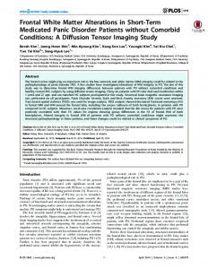
Fig. 1. Segmentation of 2 tori in a noisy synthetic tensor field: [Top Left] Initial data [Top Right] Final segmentation [Bottom] Surface evolution

A Riemannian Approach to Diffusion Tensor Images Segmentation

Fig. 2. Segmentation of the corpus callosum (A: anterior, P: posterior)

Fig. 3. Segmentation of the left corticospinal tract (I: inferior, S: superior)

599

600

C. Lenglet et al.

4.2

Synthetic Data

In order to validate the algorithm on data for which ground truth is available, we have generated a 50×50×50 synthetic tensor field composed of a background with a privileged orientation and 2 tori whose internal tensors are oriented according to the tangential direction of the principal circle of the tori. Eigenvectors and eigenvalues of the tensors are independently corrupted by Gaussian noise (figure 1). Despite the large orientational variation and the fairly high level of noise, our method is able to correctly extract the structures for different initializations. 4.3

Real Data

Diffusion weighted images were acquired on a 3 Tesla Siemens Magnetom Trio whole-body scanner. We used 12 gradients directions with a b-factor of 1000s/mm2 , T R = 9.2s and T E = 92ms. Voxel size is 2 × 2 × 2mm. The corpus callosum is a very important part of the brain that connects areas of each hemisphere together. By initializing our segmentation with only 2 small spheres within this structure, we managed to extract the volume presented on figure 2. Finally, we focused on a different part of the white matter, known as the internal capsule. Mainly oriented in the inferior-superior direction, the posterior part of this fiber bundle includes the corticospinal tract for which we present, on figure 3, the result of the segmentation obtained with our method. We also tested, on this particular example, the overall influence of the boundary term pb . It turns out that, as expected, if we do not use this term in the energy, the resulting segmentation incorporates undesired regions of the brain such as the anterior and posterior parts of the corona radiata. This shows that the interface detection part of our method does play an important role to discriminate relevant structures. Visual inspection of the results obtained on several datasets and comparison with neuroanatomical knowledge validated the proposed segmentations.

5

Conclusion

We have presented a novel statistical and geometric approach to the segmentation of diffusion tensor images seen as fields of multivariate normal distributions. We focused on the differential geometrical properties of the space of normal distributions to derive a generalized Gaussian law on that manifold. This allowed us to model the distribution of a subset of diffusion tensors. Together with a constraint on the variations of the tensor field, we have embedded this information in a statistical surface evolution framework to perform the segmentation of inner structures of the cerebral white matter. This method achieved very good results on synthetic data and was able to capture fine details in real DTI datasets. Acknowledgments. This work was supported by grants NSF-0404617 USFrance (INRIA) Cooperative Research, NIH-R21-RR019771, NIH-RR08079, the MIND Institute and the Keck foundation.

A Riemannian Approach to Diffusion Tensor Images Segmentation

601

References 1. Le Bihan, D., Breton, E., Lallemand, D., Grenier, P., Cabanis, E., Laval-Jeantet, M.: MR imaging of intravoxel incoherent motions: Application to diffusion and perfusion in neurologic disorders. Radiology (1986) 401–407 2. Basser, P., Mattiello, J., Le Bihan, D.: MR diffusion tensor spectroscopy and imaging. Biophysica (1994) 259–267 3. Tschumperl´e D., Deriche, R.: Variational frameworks for DT-MRI estimation, regularization and visualization. In: Proc. ICCV (2003) 116–122 4. Mori, S., Crain, B., Chacko, V., Zijl, P.V.: Three-dimensional tracking of axonal projections in the brain by magnetic resonance imaging. Annals of Neurology 45 (1999) 265–269 5. Behrens, T., Johansen-Berg, H., Woolrich, M., Smith, S., Wheeler-Kingshott, C., Boulby, P., Barker, G., Sillery, E., Sheehan, K., Ciccarelli, O., Thompson, A., Brady, J., Matthews, P.: Non-invasive mapping of connections between human thalamus and cortex using diffusion imaging. Nat. Neuroscience 6 (2003) 750–757 6. Lenglet, C., Deriche, R., Faugeras, O.: Inferring white matter geometry from diffusion tensor MRI: Application to connectivity mapping. In: Proc. ECCV (2004) 127–140 7. Corouge, I., Gouttard, S., Gerig, G.: A statistical shape model of individual fiber tracts extracted from diffusion tensor MRI. In: Proc. MICCAI (2004) 671–679 8. Zhukov, L., Museth, K., Breen, D., Whitaker, R., Barr, A.: Level set segmentation and modeling of DT-MRI human brain data. Journal of Electronic Imaging 12:1 (2003) 125–133 9. Wiegell, M., Tuch, D., Larson, H., Wedeen, V.: Automatic segmentation of thalamic nuclei from diffusion tensor magnetic resonance imaging. NeuroImage 19 (2003) 391–402 10. Feddern, C., Weickert, J., Burgeth, B., Welk, M.: Curvature-driven PDE methods for matrix-valued images. Technical Report 104, Department of Mathematics, Saarland University, Saarbr¨ ucken, Germany (2004) 11. Rousson, M., Lenglet, C., Deriche, R.: Level set and region based surface propagation for diffusion tensor MRI segmentation. In: Proc. Computer Vision Approaches to Medical Image Analysis, ECCV Workshop (2004) 123–134 12. Wang, Z., Vemuri, B.: Tensor field segmentation using region based active contour model. In: Proc. ECCV (2004) 304–315 13. Wang, Z., Vemuri, B.: An affine invariant tensor dissimilarity measure and its application to tensor-valued image segmentation. In: Proc. CVPR (2004) 228–233 14. Lenglet, C., Rousson, M., Deriche, R.: Segmentation of 3D probability density fields by surface evolution: Application to diffusion MRI. In: Proc. MICCAI (2004) 18–25 15. Jonasson, L., Bresson, X., Hagmann, P., Cuisenaire, O., Meuli, R., Thiran, J.: White matter fiber tract segmentation in DT-MRI using geometric flows. Medical Image Analysis (2004) In press. 16. Lenglet, C., Rousson, M., Deriche, R., Faugeras, O.: Statistics on multivariate normal distributions: A geometric approach and its application to diffusion tensor MRI. Research Report 5242, INRIA (2004) 17. Rao, C.: Information and accuracy attainable in the estimation of statistical parameters. Bull. Calcutta Math. Soc. 37 (1945) 81–91 18. Burbea, J., Rao, C.: Entropy differential metric, distance and divergence measures in probability spaces: A unified approach. Journal of Multivariate Analysis 12 (1982) 575–596

602

C. Lenglet et al.

19. Skovgaard, L.: A Riemannian geometry of the multivariate normal model. Technical Report 81/3, Statistical Research Unit, Danish Medical Research Council, Danish Social Science Research Council (1981) 20. Burbea, J.: Informative geometry of probability spaces. Expositiones Mathematica 4 (1986) 347–378 21. Eriksen, P.: Geodesics connected with the fisher metric on the multivariate manifold. Technical Report 86-13, Inst. of Elec. Systems, Aalborg University (1986) 22. Calvo, M., Oller, J.: An explicit solution of information geodesic equations for the multivariate normal model. Statistics and Decisions 9 (1991) 119–138 23. F¨ orstner, W., Moonen, B.: A metric for covariance matrices. Technical report, Stuttgart University, Dept. of Geodesy and Geoinformatics (1999) 24. Moakher, M.: A differential geometric approach to the geometric mean of symmetric positive-definite matrices. SIAM J. Matrix Anal. Appl. 26:3 (2005) 735–747 25. Fletcher, P., Joshi, S.: Principal geodesic analysis on symmetric spaces: Statistics of diffusion tensors. In: Proc. Computer Vision Approaches to Medical Image Analysis, ECCV Workshop (2004) 87–98 26. Pennec, X., Fillard, P., Ayache, N.: A Riemannian framework for tensor computing. Research Report 5255, INRIA (2004) 27. Atkinson, C., Mitchell, A.: Rao’s distance measure. Sankhya: The Indian Journal of Stats. 43 (1981) 345–365 28. Karcher, H.: Riemannian centre of mass and mollifier smoothing. Comm. Pure Appl. Math 30 (1977) 509–541 29. Pennec, X.: Probabilities and statistics on Riemannian manifolds: A geometric approach. Research Report 5093, INRIA (2004) 30. Charpiat, G., Faugeras, O., Keriven, R.: Approximations of shape metrics and application to shape warping and shape statistics. Research Report 4820, INRIA (2003) 31. Rousson, M.: Cues integrations and front evolutions in image segmentation. PhD thesis, Universit´e de Nice-Sophia Antipolis (2004) 32. Leclerc, Y.: Constructing simple stable description for image partitioning. International Journal of Computer Vision 3 (1989) 73–102 33. Zhu, S., Yuille, A.: Region competition: Unifying snakes, region growing, and Bayes/MDL for multiband image segmentation. IEEE Transactions on Pattern Analysis and Machine Intelligence 18 (1996) 884–900 34. Paragios, N., Deriche, R.: Geodesic active regions: a new paradigm to deal with frame partition problems in computer vision. Journal of Visual Communication and Image Representation 13 (2002) 249–268 35. Osher, S., Sethian, J.: Fronts propagating with curvature dependent speed: Algorithms based on the Hamilton-Jacobi formulation. Journal of Computational Physics 79 (1988) 12–49 36. Chan, T., Vese, L.: Active contours without edges. IEEE Transactions on Image Processing 10 (2001) 266–277 37. Zhao, H., Chan, T., Merriman, B., Osher, S.: A variational level set approach to multiphase motion. Journal of Computational Physics 127 (1996) 179–195 38. Caselles, V., Kimmel, R., Sapiro, G.: Geodesic active contours. The International Journal of Computer Vision 22 (1997) 61–79 39. Kass, M., Witkin, A., Terzopoulos, D.: Snakes: Active contour models. In: Proc. ICCV (1987) 259–268 40. Rousson, M., Deriche, R.: A variational framework for active and adaptative segmentation of vector valued images. In: Proc. IEEE Workshop on Motion and Video Computing (2002) 56–62