micromachines Article
A Robot-Assisted Cell Manipulation System with an Adaptive Visual Servoing Method Yu Xie 1 , Feng Zeng 1 , Wenming Xi 1 , Yunlei Zhou 1 , Houde Liu 2, * and Mingliang Chen 3 1 2 3
*
School of Aerospace Engineering, Xiamen University, Xiamen 361005, China;
[email protected] (Y.X.);
[email protected] (F.Z.);
[email protected] (W.X.);
[email protected] (Y.Z.) Shenzhen Engineering Laboratory of Geometry Measurement Techinology, Graduate School at Shenzhen, Tsinghua University, Shenzhen 518055, China Key Laboratory of Marine Biogenetic Resources, Third Institute of Oceanography, State Oceanic Administration, Xiamen 361005, China;
[email protected] Correspondence:
[email protected]; Tel.: +86-132-4665-8090
Academic Editors: Aaron Ohta and Wenqi Hu Received: 10 May 2016; Accepted: 15 June 2016; Published: 20 June 2016
Abstract: Robot-assisted cell manipulation is gaining attention for its ability in providing high throughput and high precision cell manipulation for the biological industry. This paper presents a visual servo microrobotic system for cell microinjection. We investigated the automatic cell autofocus method that reduced the complexity of the system. Then, we produced an adaptive visual processing algorithm to detect the location of the cell and micropipette toward the uneven illumination problem. Fourteen microinjection experiments were conducted with zebrafish embryos. A 100% success rate was achieved either in autofocus or embryo detection, which verified the robustness of the proposed automatic cell manipulation system. Keywords: cell manipulation; robotics; adaptive imaging processing; autofocusing
1. Introduction Microinjecting microliters of genetic material into embryos of model animals is a standard method used for analyzing vertebrate embryonic development and the pathogenic mechanisms of human disease [1,2]. Cell micromanipulation procedure is currently being conducted manually by trained personnel. This requires lengthy training and lack of reproducibility. However, this method cannot meet the demands of the growing development of biological research and the need for testing materials [3]. The integration of robotic technology into biological cell manipulation is an emerging research area that endeavors to improve efficiency, particularly in precision and high throughput aspects. Recently, several robotic injection prototypes for cell microinjection were reported [4–9]. Wang et al. used a position control strategy to inject zebrafish embryos, in which a visual servoing method was used to detect the target position of the end-effector, and a PID (proportional-integral-derivative) position control was used for micropipette movement [4]. Position control with force signal feedback was used by Lu et al. to inject zebrafish embryos, where a piezoresistive microforce sensor was used to monitor the injection process [5]. A homemade PVDF (Poly vinylidene fluoride) microforce sensor was proposed in [6] to evaluate the haptic force in a cell injection process. Huang et al. used vision and force information to determine three-dimensional cell microinjection, and adopted an impedance control method to control the movement of the injector in the z-direction [7]. Xie et al. employed an explicit force control method to regulate the cell injection force on zebrafish embryos [8,9]. However, two problems remained unsolved. First, these studies focused on the motorized injection strategy and control algorithm, even though vision feedback was adopted in every robotic prototype. Past studies Micromachines 2016, 7, 104; doi:10.3390/mi7060104
www.mdpi.com/journal/micromachines
Micromachines 2016, 7, 104
2 of 15
Micromachines 2016, 7, 104
2 of 15
did not focus on visual feedback in these robotic injection systems. The segmentation of the embryo and injection systems. The segmentation of the embryo and injection pipette is relatively easy for a fixed injection pipette is relatively easy for a fixed image. Since invention of automatic microinjection used for image. Since invention of automatic microinjection used for large-scale batch microinjections, one of large-scale batch microinjections, one of the main challenges lies in the quality of the real-time images the main challenges lies in the quality of the real-time images that are affected by the environment that are affected by the environment (i.e., uneven illumination), cell culture medium or individual (i.e., uneven illumination), cell culture medium or individual cell morphology. Therefore, we cell morphology. Therefore, we focused on adaptive and robust image processing in our visual servo focused on adaptive and robust image processing in our visual servo system design. system design. Second, in addition to automating the embryo injection process, a smart visual servoing Second, in addition to automating the embryo injection process, a smart visual servoing structure structure is able to improve the automation level and simplify the whole manipulation system. For is able to improve the automation level and simplify the whole manipulation system. For instance, a instance, a microscope autofocusing system can bring the samples into focus by using the focus microscope autofocusing system can bring the samples into focus by using the focus algorithm and algorithm and motion control. To date, no studies concentrated on the autofocusing method for a motion control. To date, no studies concentrated on the autofocusing method for a robot-assisted robot-assisted zebrafish embryo microinjection. zebrafish embryo microinjection. Section 2 of this paper introduces the architecture of the visual servoing cell microinjection Section 2 of this paper introduces the architecture of the visual servoing cell microinjection robot system. Section 3 reports on the microscope automatic servoing method used to automate the robot system. Section 3 reports on the microscope automatic servoing method used to automate cell manipulation process. The suitability of different focus criteria was evaluated and a visual the cell manipulation process. The suitability of different focus criteria was evaluated and a visual servoing motion control method is described for a robotic embryo microinjection system. An servoing motion control method is described for a robotic embryo microinjection system. An adaptive adaptive visual processing algorithm developed for real-time cell and micropipette location under visual processing algorithm developed for real-time cell and micropipette location under different different illumination environments is discussed. Finally, Sections 4 and 5 report the experimental illumination environments is discussed. Finally, Sections 4 and 5 report the experimental results and results and discussion of zebrafish embryos microinjection. discussion of zebrafish embryos microinjection.
2. 2. The TheAutomatic AutomaticMicroinjection MicroinjectionSystem System 2.1. 2.1. System System Configuration Configuration The visual servo servo cell cellmicroinjection microinjectionsystem systemincluded: included:(a)(a)a microscope a microscope vision processing part; The visual vision processing part; (b) (b) a micromanipulation part; (c)integrated an integrated interface software platform for visual servoing. a micromanipulation part; andand (c) an interface software platform for visual servoing. The The block diagram of system the system is shown in Figure 1. The photograph microinjection system block diagram of the is shown in Figure 1. The photograph of of thethe microinjection system is is shown in Figure 2. shown in Figure 2.
Figure 1. Block diagram of the automatic cell microinjection system.
Figure 1. Block diagram of the automatic cell microinjection system.
The visual processing part was responsible for the management of the camera, image acquisition and processing. included an inverted microscope for (model: Motic Inc., Wetzlar, Germany) The visual It processing part was responsible the AE-31, management of the camera, image and a CMOS metal-oxide-semiconductor) camera (model: IDS acquisition and(complementary processing. It included an inverted microscope (model: AE-31,uEye MoticUI-1540M, Inc., Wetzlar, Inc., Obersulm, The microscope had a working distance of 70camera mm with a minimum Germany) and Germany). a CMOS (complementary metal-oxide-semiconductor) (model: uEye UI-1540M, IDS Inc., Obersulm, Germany).device) The microscope a working distance of with a step of 0.2 mm. A CCD (charge-coupled adapter ofhad 0.65ˆ and an objective of70 4ˆmm (N.A. 0.1) minimum steptoofobserve 0.2 mm. CCD (charge-coupled adapter 0.65× and an the objective of 4× were selected theAzebrafish embryos. The device) microscope was of working under bright-field (N.A. 0.1) were selected to observe the zebrafish embryos. The microscope was working the observation mode that provided the necessary optical magnification and illumination levels under for proper bright-field observation mode that provided the necessary optical magnification and illumination
Micromachines 2016, 7, 104 Micromachines 2016, 7, 104
3 of 15 3 of 15
levels forofproper imagingarea. of the area. The CMOS camera mounted onwith the amicroscope imaging the injection Theinjection CMOS camera was mounted on was the microscope resolution with a resolution of 1280 and a 25 fpsused frame rate wasthe used to acquire the video. of 1280 ˆ 1024 pixel, and ×a 1024 25 fpspixel, frame rate was to acquire video.
Figure 2. The The photograph photograph of of the automatic microinjection system.
The micromanipulation part managed the motion controlling instructions from the host The micromanipulation part managed the motion controlling instructions from the host computer computer by handling all processing and signal generation to drive the motion devices using the by handling all processing and signal generation to drive the motion devices using the serial and serial and parallel ports. A three-degrees-of-freedom (3-DOF) robotic arm with a 0.04 μm parallel ports. A three-degrees-of-freedom (3-DOF) robotic arm with a 0.04 µm positioning resolution positioning resolution (model: MP-285, Sutter Inc., Novato, CA, USA) was used to conduct the (model: MP-285, Sutter Inc., Novato, CA, USA) was used to conduct the automatic microinjection task. automatic microinjection task. To determine the visual servoing automatic microinjection, an integrated software platform To determine the visual servoing automatic microinjection, an integrated software platform was necessary to confirm communications among function modules of the image acquisition, image was necessary to confirm communications among function modules of the image acquisition, image processing, automatic focusing and automatic microinjection. Because the microinjection system was processing, automatic focusing and automatic microinjection. Because the microinjection system manipulated from a host computer, a graphical user interface (GUI) was also required to enable the was manipulated from a host computer, a graphical user interface (GUI) was also required to enable interaction between the user and cell micro-world. More details about the software platform are the interaction between the user and cell micro-world. More details about the software platform are introduced in the next subsection. introduced in the next subsection. 2.2. Integrated Interface Software Platform for Visual Servoing 2.2. Integrated Interface Software Platform for Visual Servoing The integrated interface software platform for visual servoing control was developed under the The integrated software platform servoingand control was developed the Microsoft Visual C++interface (6.0) environment to ensurefor thevisual compatibility portability among theunder software Microsoft Visual C++ (6.0) to ensure the compatibility and portability amongused the modulus and hardware. Forenvironment image acquisition, the camera Software Development Kit (SDK) software modulus and hardware. For image acquisition, the camera Software Development Kit C and a small amount of C++ programming, which is compatible with Microsoft Visual C++. For (SDK) usedprocessing C and a small amountthe of Intel C++ programming, which is compatible Microsoft Visual the image algorithm, OpenCV image processing library with was used, which also C++. For the image processing algorithm, the Intel OpenCV image processing library was used, is compatible with Microsoft Visual C++. The 3-DOF manipulator was controlled by a commercial which is compatible Microsoft Visual The 3-DOF by a motionalso controller and waswith connected to the hostC++. computer by an manipulator RS-232 serial was port.controlled The Windows commercial motion controller and was connected to the host and computer anposition RS-232 serial port. The API (Application Programming Interface) was used to send receivebythe information of Windows API (Application Programming Interface) was used to send and receive the position the manipulator. information of the manipulator. A GUI was designed to provide an interactive way to conduct the robot-assisted microinjection A GUI was designed to an visual interactive waymicroinjection to conduct theinteractive robot-assisted microinjection procedure. Figure 3 shows theprovide designed servoing interface developed procedure. Figure 3 shows the designed visual servoing microinjection interactive interface with the MFC (Microsoft Foundation Classes) framework. The functions of the buttons are described developed in Table 1. with the MFC (Microsoft Foundation Classes) framework. The functions of the buttons are described in Table 1.
Micromachines 2016, 7, 104 Micromachines 2016, 7, 104
4 of 15 4 of 15
Figure 3. Visual servoing microinjection interactive interface. Figure 3. Visual servoing microinjection interactive interface. Table 1. The button functions of the user interface. Table 1. The button functions of the user interface.
Buttons Buttons StartStart LiveLive StopStop LiveLive Image SaveSave Image Cell Autofocus Cell Autofocus
Functions Functions Open theOpen camera, and display live video in the picture box the camera, and display live video in the picture box Stopand video and display current image in the picture box Stop video display current image in the picture box an image the specified location Save anSave image to thetospecified location Begin automatic cell autofocusing manipulation automatic cellmicropipette autofocusing manipulation BeginBegin to search the cell and by visual processing algorithm and Image Process Begin to search the results cell and micropipette processing show in the picture box by andvisual corresponding infoalgorithm blocks Image Process Cell Auto Microinject Beginresults to automatically move the and conduct microinjection and show in the picture boxmicropipette and corresponding info blocks Exit Save and exit the program Cell Auto Microinject Begin to automatically move the micropipette and conduct microinjection Exit Save and exit the program
3. Visual Servoing Algorithm for Automatic Cell Microinjection 3. Visual Servoing Algorithm for Automatic Cell Microinjection 3.1. Visual Servoing Algorithm for Automatic Cell Autofocusing
3.1. Visual Servoing Algorithm for Automatic Cell Autofocusing 3.1.1. Selection of the Criterion Function 3.1.1.Since Selection of the Criterion the system was used Function for a large-scale microinjection, speed and reliability were our primary considerations in the development of the autofocus algorithm becausespeed they enhance the efficiency Since the system was used for a large-scale microinjection, and reliability were and our level of automation for the entire system. Criterion functions were studied for the autofocusing of primary considerations in the development of the autofocus algorithm because they enhance the the microscopes and other optical instruments in prior works [10]. Eighteen focus algorithms were efficiency and level of automation for the entire system. Criterion functions were studied for the compared in [11,12], where variance were to noise while the autofocusing of the microscopes andbased other focus opticalalgorithms instruments in more prior sensitive works [10]. Eighteen focus gradient-based algorithms had where better variance performance sub-sample cases. In more our cell injection algorithms werefocus compared in [11,12], basedinfocus algorithms were sensitive to system, the image for processing is shown in Figure 3. The zebrafish embryo had a symmetric spherical noise while the gradient-based focus algorithms had better performance in sub-sample cases. In our shape and a clear background, some dampness fromin theFigure culture As such,embryo we narrowed cell injection system, the imagewith for processing is shown 3. liquid. The zebrafish had a the candidate criterion functions thebackground, following: the Brenner the Tenenbaum gradient symmetric spherical shape and a to clear with somegradient, dampness from the culture liquid.and As normalized variance the algorithms. such, we narrowed candidate criterion functions to the following: the Brenner gradient, the Tenenbaum gradient and normalized variance algorithms.
Micromachines 2016, 7, 104
5 of 15
Micromachines 2016, 7, 104
5 of 15
The Brenner gradient [13] measured the differences between a pixel value and its neighbor pixel with a vertical or horizontal distance of two pixel positions. The horizontal direction is used in this paper: The Brenner gradient [13] measured the differences between a pixel value and its neighbor pixel with a vertical or horizontal distance of two pixel positions. The horizontal direction is used in 2 f ( I ) = I ( x + 2, y ) − I ( x , y ) [ ] (1) this paper: ) ÿx ÿy ! 2, rIpx ` 2, yq ´ Ipx, yqs , f pIq “ (1) x the y pixel at ( x, y ) . where I ( x, y) was a gray-level intensity of
{
}
The Tenenbaum gradientintensity (Tenengrad) [14] was gradient magnitude maximization algorithm where Ipx, yq was a gray-level of the pixel atapx, yq. that calculated the sum of the squared values of the vertical Sobel operators: The Tenenbaum gradient (Tenengrad) [14] washorizontal a gradientand magnitude maximization algorithm that calculated the sum of the squared values of the horizontal and vertical Sobel operators: f ( I ) = S x ( x, y)2 + S y ( x, y)2 (2) ! ) ÿx ÿy , f pIq “ Sx px, yq2 ` Sy px, yq2 , (2) x y where S x ( x, y) and S y ( x, y ) were the horizontal and vertical Sobel operators.
{
}
The normalized variance the differences the operators. pixel values and the mean pixel where Sx px, yq and Sy px, yq werequantified the horizontal and vertical in Sobel value:The normalized variance quantified the differences in the pixel values and the mean pixel value:
1 f ( I ) = 1 ÿ ( f x , y − μ ) 22 f pIq “ μ p f x,y ´ µq , x, y µ x,y ,
(3) (3)
where μ was the mean pixel value of the image defined in Equation (4). where µ was the mean pixel value of the image defined in Equation (4). 1 ÿ I ( x, y ) μ= 1ÿ µ “ N x y Ipx, yq. . N x
(4) (4)
y
With selected focus focus function, function, the With aa selected the corresponding corresponding focus focus curve curve was was obtained obtained for for the the captured captured images along the complete focus interval. Figure 4 shows the normalized focus curves of images along the complete focus interval. Figure 4 shows the normalized focus curves of each each image, image, of which the step length is 200 μm. Different curves arrived at their global peak at the same of which the step length is 200 µm. Different curves arrived at their global peak at the same z-position. z-position. All three curves correctly represented the focal plane. Some local maxima were observed All three curves correctly represented the focal plane. Some local maxima were observed with the with the normalized may the prevent the autofocusing fromthe finding normalized gradient gradient function.function. This mayThis prevent autofocusing algorithmalgorithm from finding focal the focal plane or increasing the computational complexity. When compared to the Tenengrade plane or increasing the computational complexity. When compared to the Tenengrade gradient and gradient and thevariance normalized variance function,function the Brenner function exhibited a more peak, the normalized function, the Brenner exhibited a more narrow peak, narrow which meant which meant good reproducibility and better searching for the focus plane. good reproducibility and better searching for the focus plane. 1
Normalized Focus Measure
0.95
0.9
0.85
0.8
Tenengrade gradient Brenner gradient Normalized variance
0.75
0.7
0
2
4
6
8 10 12 14 z-position (Step Number)
16
Figure 4. 4. Focus Focus curves curves after after normalization. normalization. Figure
18
20
22
Micromachines 2016, 7, 104
6 of 15
Another evaluation criterion for the real-time visual processing system is the computational time of the focus function. A summary of the computational time required to process 23 images is presented in Table 2. The Brenner gradient function took the least time when compared to the other two functions. Table 2. Computational time for three selected focus functions. Functions
Tenengrade Gradient Function
Brenner Gradient Function
Normalized Variance Function
Computational Times (s)
1.2794
0.69279
1.0831
Therefore, the Brenner function was chosen as the criteria function for the zebrafish embryos autofocus algorithm. 3.1.2. Implementation of the Automatic Focusing Method We used an eyepiece with a magnifying power of 10ˆ, the objective of 4ˆ, and a numerical aperture of 0.1. The following equation was used to calculate the depth of field: DF “
10´3 λ , ` 7AM 2A2
(5)
where DF was the depth of field, A was the numerical aperture, M was the total magnification, λ was Micromachines 2016, 7, and 104 the depth of field was DF = 63.2 µm. 7 of 15 the light wavelength
Figure 5. Control method schematic of the entire automatic focusing process. lized Focus Measure
Figure 5. Control method schematic of the entire automatic focusing process. 1 0.8
0.6
Micromachines 2016, 7, 104
7 of 15
Normolized Focus Measure
If the automatic step length was larger than the depth of field, then the cells may move out of the depth of microscope field. Therefore, the step length must be smaller than DF . To increase the speed of the focusing time, a two-phase automatic focusing method was developed, where a step length of 200 µm was used for coarse focus and 50 µm was used for fine focus. In the coarse focusing phase, the immediate sharpness evaluation value was compared with the previous two images to determine if value was incremental, which would indicate that the manipulator was moving towards the focal plane. If the sharpness evaluation value was not incremental, then it was compared with the previous two images to see if it diminished, which would indicate that the image was out-of-focus. If it was diminished, we began the fine tuning phase, in which the manipulator moved back with a step of fine tuning, similar to the coarse tuning. The control flow of the whole automatic focusing is depicted in Figure 5. With the Brenner focus function, the corresponding sharpness evaluation value was obtained for the captured images along the complete focus interval. Figure 6a is the coarse focusing curve with a length of 200 µm after normalization. The curve peaked at step 28, which meant it was close to the focal plane. Next, we used a fine focus at step 30 that was also marked as step 0 in the fine focusing stage. The fine focusing curve arrived at a global peak at step 6 that indicated the location of the focal plane, as shown in Figure 6b. The computational time for the Brenner gradient function to process the 31 images in coarse focusing was 0.92786 s, while the time for nine images in fine focusing was 0.23155 s. Figure 5. Control method schematic of the entire automatic focusing process. 1 0.8
0.6
0.4
0
5
10
15 20 z-position (Step No.)
25
30
Normolized Focus Measure
(a) 1 0.9
0.8
0.7
0
1
2
3 4 5 z-position (Step No.)
6
7
8
(b) Figure 6. 6. Focusing focusing with a step length of Figure Focusing curves curveswith withBrenner Brennergradient gradientfunction: function:(a)(a)coarse coarse focusing with a step length 200 μm; and (b) fine focusing with a step length of 50 μm. of 200 µm; and (b) fine focusing with a step length of 50 µm.
3.2. Adaptive Image Processing Algorithm for Automatic Cell and Pipette Detection This section provides real-time location information about the embryo and the injection pipette for the automatic microinjection system. The tasks include (a) detecting and locating the embryo; (b) detecting and locating the injection pipette; and (c) automatically moving the injection pipette to the center of yolk under visual servo. In a real-time automatic cell microinjecting system, one of the primary challenges is the quality of the images affected by the environment (i.e., uneven illumination), cell culture medium or cell morphology. Our algorithm focused on adaptive and robust image processing.
for the automatic microinjection system. The tasks include (a) detecting and locating the embryo; (b) detecting and locating the injection pipette; and (c) automatically moving the injection pipette to the center of yolk under visual servo. In a real-time automatic cell microinjecting system, one of the primary challenges is the quality of the images affected by the environment (i.e., uneven Micromachines 2016,cell 7, 104culture medium or cell morphology. Our algorithm focused on adaptive 8 ofand 15 illumination), robust image processing. 3.2.1. 3.2.1.Real RealTime TimeAdaptive-Threshold Adaptive-ThresholdDetection Detectionfor forAutomatic AutomaticCell CellDetection Detection The Thebinary binaryoperation operationisisaaclassical classicalthreshold thresholdsegmentation segmentationmethod methodtotoseparate separateobjects objectsof ofinterest interest from the background. A conventional binary operation method uses a constant threshold T throughout from the background. A conventional binary operation method uses a constant threshold T the whole image. Some image. methods havemethods been proposed to automatically the value, such the as throughout the whole Some have been proposed tocalculate automatically calculate the Mean Technique [15], the P-Tile Method [16], the Iterative Threshold Selection [17] and Otsu’s value, such as the Mean Technique [15], the P-Tile Method [16], the Iterative Threshold Selection [17] method [18].method Figure 7[18]. illustrates binary operation results using Otsu’s The conventional and Otsu’s Figurethe 7 illustrates the binary operation resultsmethod. using Otsu’s method. The threshold was threshold efficient for theefficient uniformfor illumination but was not ideal theideal illumination conventional was the uniformimages illumination images but when was not when the was uneven. was uneven. illumination
(a)
(b)
(c)
(d)
Figure 7. Results of conventional threshold: even illumination (left); uneven illumination (right). Figure 7. Results of conventional threshold: even illumination (left); uneven illumination (right). (a) Original image (even illumination); (b) Binary image with Otsu’s method (even illumination); (a) Original image (even illumination); (b) Binary image with Otsu’s method (even illumination); (c) Original image (uneven illumination); (d) Binary image with Otsu’s method (uneven (c) Original image (uneven illumination); (d) Binary image with Otsu’s method (uneven illumination). illumination).
The video images in in thethe automatic injection experiments, so the shadows or Theimages imageswere werereal-time real-time video images automatic injection experiments, so the shadows the direction of illumination may cause uneven illumination. Non-adaptive methods that analyze the or the direction of illumination may cause uneven illumination. Non-adaptive methods that analyze histogram of the of entire unsuitable. An adaptive is proposed the histogram the image entireare image are unsuitable. Anthreshold adaptivecalculating threshold method calculating methodtois specify an adaptive threshold for every pixel in an image. We defined the adaptive threshold as: proposed to specify an adaptive threshold for every pixel in an image. We defined the adaptive
threshold as:
Tij “ Aij ´ param1, (6) Tij = Aij − param1 (6) , where A was the weighted average gray value of pixels in the region around a particular pixel. The where A was theregion weighted average grayby value of pixelsofinb the around a particular pixel. The block size of the was represented parameters andregion param1. In this algorithm, pixels with gray value S larger than their threshold Tij were set to 255, and ij block size of the region was represented by parameters of b and param1. all others were set to 0.pixels A circulation the Stwo parameters was used to adjust the threshold Tij In this algorithm, with grayfor value ij larger than their threshold Tij were set to 255, and all to segment the cell membrane, yolk and background from uneven illumination images. The flow others were set to 0. A circulation for the two parameters was used to adjust the threshold Tij to diagram of the circulation to optimize the two parameters is shown in Figure 8. After the segment the cell membrane, yolk and background from uneven illumination images. adaptive The flow threshold obtained, a regular least squared based ellipse fitting method [19] was usedthe to find the diagram of the circulation to optimize the two parameters is shown in Figure 8. After adaptive embryo. The contours of the image are detected and every contour is saved in the form of pixel threshold obtained, a regular least squared based ellipse fitting method [19] was used to find the coordinates’ of the points. Then, pointsand in every which embryo. Thevectors contours of the image are the detected everycontour contourare is fitted savedtointhe theellipse, form of pixel iscoordinates’ computed by minimizing the sum of the squares of the distances of the given points to an ellipse. vectors of the points. Then, the points in every contour are fitted to the ellipse, which is Then, the length of the major axis of the fitted ellipse, was used to of tellthe if the identified Tij computed by minimizing the sum of the squares ofL,the distances given points threshold to an ellipse. isThen, suitable. the length of the major axis of the fitted ellipse, L, was used to tell if the identified threshold Tij The adaptive-threshold detection method processed different video images in real-time and had is suitable. good adaptability in both images with uniform illumination and uneven illumination, as shown in Table 3. If the image has more uneven illumination, a bigger block size is required to determine the ellipse (embryo). A green oval was used to mark the embryonic membrane, and a red dot was used to mark the embryo center. The results of our experiments showed that the proposed method can effectively detect edge of the embryo and adaptively locate the embryo center.
Then, length major axis fitted ellipse, was used tell if the identified threshold Then, thethe length ofof thethe major axis ofof thethe fitted ellipse, L, L, was used toto tell if the identified threshold TijTijij suitable. is is suitable. Begin Begin
Micromachines 2016, 7, 104 Micromachines 2016, 7, 104
: The result of Rijij :R result of adaptive-threshold ij RThe result of adaptive-threshold adaptive-threshold ij : The operation of pixel (i, operation of the pixel (i, j). operation of the the pixel (i, j). j).
Initialize (b=5 Initialize (b=5 param1=5) param1=5)
9 of 15 9 of 15
:: distance measured in L :L measured in pixels. Ldistance distance measured in pixels. pixels.
Adaptive threshold Adaptive threshold operation: operation: = 255, Sij>T Sijij>T ij ij Rij R=ijij 255, ij others Rij R=ijij0,= 0,others Following image Following image processing processing Fitting ellipses Fitting ellipses of of thethe embryo least embryo byby least squares method and squares method and saving major axis saving thethe major axis of of max ellipse thethe max ellipse to to a a various various L L 300