A Robotic Validation of the Attractive Field Model: An Inter-Disciplinary Model of Self-Regulatory Social Systems Md Omar Faruque Sarker and Torbjørn S. Dahl Robotic Intelligence Lab, University of Wales, Newport, UK Mdomarfaruque.Sarker|
[email protected]
Abstract. Division of labour in multi-robot systems or multi-robot task allocation (MRTA) is a challenging research issue. We propose to solve this MRTA problem using a set of previously published generic rules for division of labour derived from the observation of ant, human and robotic social systems. These bottom-up rules describe the phenomenon of selfregulated division of labour in terms of attractive fields between robots and tasks. The concrete form of these rules, the attractive filed model, avoids the strong dependence on local interactions found in many existing approaches to MRTA. We present experimental results that constitute a first validation of attractive filed model as a mechanism for MRTA and as a multi-disciplinary model of self-organisation in social systems. Our experiments used 16 e-puck robots in a 2m x 2m area.
1
Introduction
Scientific studies show that a large number of animal as well as human social systems grow, evolve and generally continue functioning well by the virtue of their individual self-regulatory mechanism of division of labour (DOL) [2]. This has been accomplished without any central authority or any explicit planning and coordinating element. Indirect communication such as stigmergy is instead used to exchange information among individuals. In robotics, multi-robot task allocation (MRTA) is a common research challenge [4]. It is generally identified as the problem of assigning tasks to appropriate robots at appropriate times considering the potential changes in the environment and/or the performance of the robots. MRTA is an optimal assignment problem that has been shown to be NP-hard, so optimal solutions can not be expected for large problems [8]. In addition to the inherent complexity of MRTA, the problem is also commonly restricted to avoid central planners or coordinators for task assignments. The robots are also commonly limited to local sensing, communication and interaction [5] where no single robot has complete knowledge of the past, present or future actions of other robots or a complete view of the world state. Traditionally MRTA solutions are broadly divided into two major categories: 1) Predefined and 2) Bio-inspired self-organized task-allocation [9]. Early research on predefined task-allocation was dominated by intentional coordination,
2
M. O. F. Sarker and T. S. Dahl
use of dynamic role assignment [8] and market-based bidding approach [3]. Under these approaches, robots use direct task-allocation method to communicate and to negotiate tasks. These approaches are intuitive, comparatively straightforward to design and implement and can be analysed formally. However, these approaches typically works well only when the number of robots are small (≤ 10). The self-organized task-allocation, on the other hand, relies on the emergence of group behaviours, e.g., emergent cooperation [5], adaptive mechanisms such as adaptation rules [6]. These approaches typically handle systems with local sensing, local interactions and typically little or no explicit communications or negotiations among robots. self-organized systems are more scalable and robust due to their inherent parallelism and redundancy. However, in these systems, solutions are unintuitive and thus difficult to design, analyse formally and implement practically [4, 5]. The solutions found by these systems are typically sub-optimal and, as emergence is a result of interactions among robots and their environment, it is also difficult to predict exact behaviours of robots and overall system performance. The current challenges in self-organized task allocation approaches have motivated us to look for a suitable alternative. In nature we find that task allocation in animal or insect societies can be governed by non-centralized rules and that they are self-regulating and self-stabilizing [2]. As a part of a collaborative project, we have studied the behaviours of ants, humans and robots and, from a set of generic rules of self-regulation, we have developed the attractive field model (AFM). This has become a common formal model of division of labour in social systems [1]. In this paper, we present an application of AFM in a robotic system. Section 2 presents AFM with its generic and robotic interpretations. It also presents an application of AFM in a manufacturing shop-floor scenario. Section 3 introduces our implementation of MRTA. Section 4 presents the design of our experiments including specific parameters and observables. Section 5 discusses our experimental results and section 6 draws conclusions.
2 2.1
The Attractive Field Model Generic Interpretation
AFM provides an abstract framework for self-regulatory DOL in social systems [1]. In order to achieve self-regulation, it proposes four generic rules: continuous flow of information, concurrency, learning and forgetting, all of them will be explained later. In terms of networks, the model is a bipartite network, meaning that there are two different types of nodes. One set of nodes describes the sources of the attractive fields and the other set describes the agents. Links only exist between different types of nodes and they encode the flow of information so that, even if there is no direct link between two agents, their interaction is taken into account in the information flow. The strength of the field depends on the distance between the task and the agent. This relationship is represented using weighted links. In addition, there is a permanent field that represents the no-task option.
Robotic Validation of the Attractive Field Model
3
The model can be mapped to a network as shown in Fig. 1. The correspondence is given below: 1. Source nodes (o) are tasks that can be divided between a number of agents. 2. Agent nodes (x) are robots. 3. The attractive fields correspond to stimuli to perform a task, and these are encoded in a system-wide continuous flow of information. These are given by the black solid lines. 4. When an agent performs a task, the link is of a different sort, and this is denoted in the figure by a dashed line. Agents linked to a source by a red line are the robots currently doing that task. 5. The field of ignoring the information (w) corresponds to the stimulus to random walk, i.e. the no-task option, and this is denoted by the dotted lines in the graph. 6. Each of the links is weighted. The value of this weight describes the strength of the stimulus that the agent experiences. In a spatial representation of the model, it is easy to see that the strength of the field depends on the physical distance of the agent to the source. In addition, the strength can be increased through sensitisation of the agent via experience or learning. Similarly, when the task is not done for some time, this strength can be gradually attenuated, which can be treated as forgetting. This distance is not depicted in the network, it is represented through the weights of the links . In the figure of the network, the nodes have an arbitrary place. Note that even though the distance is physical in this case, the distance in the model applied to other systems, needs not to be physical, it can represent the accessibility to the information, the time the information takes to reach the receiver, etc. In summary, looking at the network, we see that each of the agents is connected to each of the fields. This means that even if an agent is currently involved in a task, the probability that it stops doing it in order to pursue a different task, or to random walk, is always non-zero. The weighted links express the probability of an agent to be attracted to each of the fields, considered as concurrency. 2.2
Robotic Interpretation
Now let us interpret this model within the context of our MRS. Let us consider a manufacturing shop floor scenario where N number of mobile robots are required to attend to M number of shop tasks spread over a fixed area A. Let these tasks be represented by a set of small rectangular boxes resembling to manufacturing machines. Let R be the set of robots r1 , r2 , ..., rn and J the set of tasks t1 , t2 , ..., tm . Each task tj has an associated task-urgency φj indicating its relative importance over time. If a robot attends a task tj in the xth time-step, the value of φj will decrease by an amount ∆ΦIN C in the (x+1)th time-step. On the other hand, if a task has not been served by any robot in the xth time-step, φj will increase by another amount, ∆ΦDEC , in (x+1)th time-step. In order to complete a task t1 , a robot ri needs to be within a fixed boundary Dj1 of t1 .
4
M. O. F. Sarker and T. S. Dahl X
X
X
TaskServer
X
X
O O
O
X
O
O O
R2
R1
W
X X
R3 X
O: Tasks X:Robots W: No-Task Option
Task1
Attractive Field (Stimulus) Performance of a task
Fig. 1. Attractive Filed Model (AFM)
Task2 Strong Attraction Weak Attraction TaskInfo Signal RobotStatus Signal
Fig. 2. A centralized communication scheme
If a robot completes a task tj it gets sensitised to it and this will increase the robot’s likelihood of selecting that task in the future. We call this variable the affinity of a robot ri to task tj its sensitization kji . If a robot does not do a task tj for some time, it forgets about tj and kj is decreased. According to AFM, all robots will establish attractive fields to all tasks due to the presence of a system-wide continuous flow of information. The strength of these attractive fields will vary according to the distances between robots and tasks, task-urgencies and corresponding sensitizations of robots. This is encoded in Eq. 1.
Sji = tanh{
kji φj } dij + δ
(1)
Sji Pji = P i S j j
(2)
Eq. 1 states that the stimuli of a robot ri to a particular task tj , Sji , depends on ri ’s spatial distance to tj (dij ), level of sensitization to j (kji ), and perceived urgency of that task (φj ). We use a very small constant value δ to avoid division by zero for the special case when a robot has reached a task. Since Sji is a probability function, it is chosen as a tanh in order to keep the values between 0 and 1. The probability of selecting each task has been determined by a probabilistic method outlined in Eq. 2. AFM suggests that concurrency of a self-regulatory system can be maintained by specifying at least two task options: doing a task and not doing a task. In robots, the latter can be be treated as random walking. So in any time-step a robot will choose from M+1 tasks. Let Ta be the allocated time to accomplish a task. If a robot can enter inside the task boundary within Ta time it waits there until Ta elapsed. Otherwise it will select a different task. 2.3
A Manufacturing Shop-Floor Interpretation
By extending the robotic interpretation of AFM, we can present a manufacturing shop-floor scenario where each task represents a manufacturing machine. These machines are capable of producing goods from raw materials, but they also
Robotic Validation of the Attractive Field Model
5
Start of production Production and accumulatedmaintenance work-load Initial production work-load Production completion time (End of production) No maintenancework pending ProductionMaintenance Mode
Pending maintenance work-load
Maintenance-Only Mode
Fig. 3. Manufacturing shop-floor production and maintenance cycles
require constant maintenance works for stable operations. Let Wj be a finite number of material parts that can be loaded into a machine j in the beginning of its production process and in each time-step, ωj units of material parts can be processed (ωj ≪ Wj ). So let Ωjp be the initial production workload of j which is simply: Wj /ωj unit. We assume that all machines are identical. In each time step, each machine always requires a minimum threshold number of robots, called hereafter as minimum robots per machine (µ), to meet its constant maintenance work-load, Ωjm unit. However, if µ or more robots are present in a machine for production purpose, we assume that, no extra robot is required to do its maintenance work separately. These robots, along with their production jobs, can do necessary maintenance works concurrently. For the sake of simplicity, in this paper we consider µ = 1. Now let us fit the above production and maintenance work-loads and task performance of robots into a unit task-urgency scale. Let us divide our manufacturing operation into two subsequent stages: 1) production and maintenance mode (PMM), and 2) maintenance only mode (MOM). Initially a machine starts working in PMM and does production and maintenance works concurrently. When there is no production work left, it then enters into MOM. Fig. 3 illustrates this for a single machine. Under both modes, let αj be the amount of workload occurs in a unit time-step if no robot serves a task and it corresponds to a fixed task-urgency ∆φIN C . On the other hand, let us assume that in each time-step, a robot, i, can decrease a constant workload βi by doing some maintenance work along with doing any available production work. This corresponds to a negative task urgency: −∆φDEC . So, at the beginning of production process, task-urgency, occurred in a machine due to its production work-loads, can be
6
M. O. F. Sarker and T. S. Dahl
encoded by Eq. 3.
p MM m0 ΦP j,IN IT = Ωj × ∆φIN C + φj
(3)
Here φm0 represents the task-urgency due to any initial maintenance work-load j of j. Now if no robot attends to serve a machine, at each time-step a constant maintenance workload of αjm will be added to j and that will increase its taskurgency by ∆φIN C . So, if k time steps passes without any production work being done, task urgency at k th time-step will follow Eq. 4. MM MM ΦP = ΦP j,k j,IN IT + k × ∆φIN C
(4)
However, if a robot attends to a machine and does some production works from it, there would be no extra maintenance work as we assumed that µ = 1. Rather, the task-urgency on this machine will decrease by ∆φDEC amount. If νk robots work on a machine simultaneously at time-step k, this decrease will be: νk × ∆φDEC . So in such cases, task-urgency in (k + 1)th time-step can be represented by: MM P MM ΦP − νk × ∆φDEC j,k+1 = Φj,k
(5)
MM At a particular machine j, once ΦP reaches to zero, we can say that there j,k is no more production work left and this time-step k can give us the production completion time of j, TjP M M . Average production time-steps of a shop-floor with M machines can be calculated by the following simple equation.
P MM Tavg =
M 1 X P MM T M j=1 j
(6)
P MM Tavg can be compared with the minimum number of time-steps necessary to P MM finish production works, Tmin . This can only happen in an ideal case where all robots work for production without any random walking or failure. We can get P MM Tmin from the total amount of work load and maximum possible inputs from MM all robots. If there are M machines and N robots, each machine has ΦP IN IT taskurgency, and at each time-step, robots can decrease N × ∆φDEC task-urgencies, P MM then the theoretical Tmin can be found from the following Eq. 7.
P MM Tmin =
MM M × ΦP IN IT N × ∆φDEC
(7)
P MM ζavg =
P MM P MM − Tmin Tavg P MM Tmin
(8)
P MM Thus we can define ζavg , average production completion delay (APCD) by following Eq. 8: When a machine enters into MOM, only µ robots are required to do its maintenance works in each time step. So, in such cases, if no robot serves a machine, the growth of task-urgency will follow Eq. 4. However, if νk robots are serving this machine at a particular time-step k th , task-urgency at (k + 1)th time-step can be represented by: OM M OM ΦM − (νk − µ) × ∆φDEC j,k+1 = Φj,k
(9)
Robotic Validation of the Attractive Field Model
7
OM By considering µ = 1 Eq. 9 will reduces to Eq. 5. Here, ΦM j,k+1 will correspond to the pending maintenance work-load (PMW) of a particular machine at a given time. This happens due to the random task switching of robots with a no-task option (random-walking). Interestingly, PMW will indicate the robustness of this system since higher PMW value will indicate the delay in attending maintenance works by robots. We can find the average PMW (APMW) per machine per timeOM OM step, χM (Eq. 10) and average PMW for all machines per time-step, χM avg j (Eq. 11).
OM χM = j
K 1 X M OM Φj,k K
OM χM = avg
(10)
k=1
3
M 1 X M OM χ M j=1 j
(11)
Implementation
SwisTrack Multi-robot ID-Pose Tracker GigE Camera E-puck robot (SwisTrack marker on top)
RobotPose
Task Server
Bluetooth radio link
Task Location
client 1
TaskInfo Robot Status client N
client 2
Robot Controller Client SignalListener
Experiment Arena
SignalEmitter
TaskSelector
DeviceController
Experiment Arena
Server PC
Fig. 4. Hardware and software setup
3.1
Design of our communication system
As shown in Fig. 2, in this model there exists a centralized TaskServer that is responsible for disseminating task information to robots. The contents of task information can be physical locations of tasks, their urgencies and so on. TaskServer delivers this information by emitting TaskInfo signals periodically. For example, in a wireless network it can be a message broadcast. Task-Server has another interface for catching feedback signals from robots. The RobotStatus
8
M. O. F. Sarker and T. S. Dahl
signal can be used to inform TaskServer about a robot’s current task id, its device status and so on. TaskServer uses this information to update relevant part of task information such as, task-urgency. This up-to-date information is sent in next TaskInfo signal. 3.2
Our current implementation
The major components of our implementation are a multi-robot tracking system, robot controller clients and a centralized task-server. In order to track all robots in real-time, we have used SwisTrack [7], a state of the art open-source, multiagent tracking system, with a 16-megapixel overhead GigE camera. This set-up gives us the position, heading and id of each of the robots by processing the image frames at about 1 FPS. The interaction of the hardware and software of our system is illustrated in Fig. 4. For inter-process communication (IPC), we have used D-Bus technology1 . We have developed an IPC component for SwisTrack that can broadcast id and pose of all robots in real-time over our server’s D-Bus interface. Apart from SwisTrack, we have implemented two major software modules: TaskServer and Robot Controller Client (RCC). They are developed in Python with its state of the art Multiprocessing 2 module. This python module simplifies our need to manage data sharing and synchronization among different sub-processes. As shown in Fig. 4, RCC consists of four sub-processes. SignalListener and SignalEmitter, interface with SwisTrack D-Bus Server and TaskServer respectively. TaskSelector implements AFM algorithms for task selection . DeviceController moves a robot to a target task. Bluetooth radio link is used as a communication medium between a RCC and a corresponding e-puck robot.
4
Experiment Design
In this section, we have described the design of parameters and observables of our experiments within the context of our manufacturing shop-floor scenario. These experiments are designed to validate AFM by testing the presence of division of labour, e.g. task specialization, dynamic task-switching or plasticity. 4.1
Parameters
Table 1 lists a set of essential parameters of our experiments. The initial values of task urgencies correspond to 100 units of production work-load without any maintenance work-load as outlined in Eq. 3. For task-urgency values, we choose a limit of 0 and 1, where 0 means no urgency and 1 means maximum urgency. Same applies to sensitisation as well, where 0 means no sensitisation and 1 means 1 2
http://dbus.freedesktop.org/doc/dbus-specification.html http://docs.python.org/library/multiprocessing.html
Robotic Validation of the Attractive Field Model
9
Table 1. Experimental parameters
Parameter Value Initial production work-load/machine (Ωjp ) 100 unit Task urgency increase rate (∆φIN C ) 0.005 Task urgency decrease rate (∆φDEC ) 0.0025 Initial sensitization (KIN IT ) 0.1 Sensitization increase rate (∆kIN C ) 0.03 Sensitization decrease rate (∆kDEC ) 0.01
maximum sensitisation. The following relationships are maintained for selecting task-urgency and sensitization parameters. ∆φIN C =
∆φDEC × N 2×M
(12)
∆kIN C M −1
(13)
∆kDEC =
Eq. 12 establishes the fact that task urgency will increase at a higher rate than that of its decrease. As we do not like to keep a task left unattended for a long time we choose a higher rate of increase of task urgency. This difference is set on the basis of our assumption that at least half of the expected number of robots (ratio of number of robots to tasks) would be available to work on a task. So they would produce similar types of increase and decrease behaviours in task urgencies. Eq. 13 suggests that the learning will happen much faster than the forgetting. The difference in these two rates is based on the fact that faster leaning gives a robot more chances to select a task in next time-step and thus it becomes more specialized on it. Task-Server updates task-info messages in the interval of 5s and robots stick on to a particular task for a maximum of 10s.
4.2
Observables
We have defined a set of observables to evaluate our implementation. The first two observables, the changes in task-urgencies and the changes in active worker ratios, can give us an overall view of plasticity of division labour. Our third observable is to find the changes in robot task specialization which is also an important measure of division of labour. Our last measurement is the communication load which is specific to this particular implementation and corresponds to the continuous flow of information. Within the context of our manufacturing shop-floor scenario, we measure the average production completion delay (APCD) and average pending maintenance work (APMW) as the metrics of manufacturing shop-floor performance.
10
M. O. F. Sarker and T. S. Dahl
5
Results and Discussions
Our AFM validation experiments were conducted with 16 robots, 4 tasks in an arena of 4 m2 for about 40 minutes and averaged them over five iterations. Fig. 5 shows the dynamic changes in task urgencies in one iteration. In order to describe our system’s dynamic behaviour holistically, we analyse the changes in task urgencies over time. Let φj,q be the urgency of a task j at q th time-step and φj,q+1 be the task urgency of (q + 1)th time-step. We can calculate the sum of changes in urgencies of all tasks at (q + 1)th time-step: ∆Φj,q+1 =
M X
(φj,q+1 − φj,q )
(14)
j=1
From Fig. 6 we can see that initially the sum of changes of task urgencies are towards negative direction. This implies that tasks are being served by a high number of robots. Fig. 8 shows that in production stage, when work-load is high, many robots are active in tasks and this ratio varies according to task urgency changes. Fig. 9 gives us the task specialization of five robots on Task3 in a particular run of our experiment. This shows us how our robots can specialize (learn) and de-specialize (forget) tasks over time. The de-specialization of tasks is calculated similar to Eq. 14. We have calculated the absolute sum of changes in sensitizations of all robots by the following equation. ∆Kj,q+1 =
M X
|(kj,q+1 − kj,q )|
(15)
j=1
This values of ∆K are plotted in Fig. 10. It shows that the overall rate of learning decreases and forgetting increases over time. It is a consequence of the gradually increased task specialization of robots and reduced task-urgencies over time. Fig. 7 presents the frequency of signalling task information by TaskServer. Since the duration of each time step is 50s long and TaskServer emits signal in every 2.5s, there is an average of 20 signals in each time-step. Within our manufacturing shop-floor scenario, we have got average production completion time 165 time-steps (825s) where sample size is (5 x 4) = 20 tasks, SD = 72 time-steps (360s). According to Eq. 7, our theoretical minimum production completion time is 50 time-steps (250s) assuming the non-stop task performance of all 16 robots with an initial task urgency of 0.5 for all 4 tasks and task urgency decrease rate ∆ΦDEC = 0.0025 per robot per time-step. Hence, Eq. 8 gives us APCD, ζ = 2.3 which means that our system has taken 2.3 times more time (575s) than the estimated minimum time. Besides, from the average 315 time-steps (1575s) maintenance activity of our robots per experiment run, we have got APMW, χ = 0.012756 which corresponds to the pending work of 3 time-steps (15s) with sample-size = 20 tasks, SD = 13 time-steps (65s), where ∆ΦIN C = 0.005 per task per time-step. This tells us the robust task performance of our robots which can return to an abandoned task within a minute or so.
Robotic Validation of the Attractive Field Model
Fig. 5. Dynamic task-urgency changes.
11
Fig. 6. Shop-floor workload history
22.0 21.5
No of Emitted Signals
21.0 20.5 20.0 19.5 19.0 18.5 18.00
10
20 30 Time Step (s)
40
50
Fig. 7. Task server’s task-info broadcasts
Fig. 8. Self-organized task-allocation
Sum of Robot Sensitization Changes
1.2 1.0 0.8 0.6 0.4 0.2 0.00
Fig. 9. Task specialization on Task3
10
20 30 Time Step (s)
40
Fig. 10. Changes in sensitizations
50
12
6
M. O. F. Sarker and T. S. Dahl
Conclusion and Future work
In this paper we have validated an inter-disciplinary generic model of selfregulated division of labour or multi-robot task allocation by incorporating it in our multi-robot system under a manufacturing shop-floor scenario. A centralized communication system has been instantiated to realize this model. We have evaluated various aspects of this model, such as the ability to meet dynamic task demands, individual robot’s task specializations, system-wide communication loads and flexibility in concurrent task completions. A set of metrics has been proposed to observe the division of labour in this system. From our experimental results, we have found that our attractive filed model can meet the requirements of dynamic division of labour by the virtue of its self-regulatory behaviours. In the future, we plan to extend this work using various local peerto-peer communication models in a multi-robot system having about 40 e-puck robots.
Acknowledgements. This research has been funded by the Engineering and Physical Sciences Research Council (EPSRC), UK, grant reference EP/E061915/1.
References 1. Arcaute, E., Christensen, K., Sendova-Franks, A., Dahl, T., Espinosa, A., Jensen, H.J.: Division of labour in ant colonies in terms of attractive fields. In: Ecol. Complex (2008) 2. Bonabeau, E., Dorigo, M., Theraulaz, G.: Swarm intelligence: from natural to artificial systems. Oxford University Press (1999) 3. Dias, M.B., Zlot, R.M., Kalra, N., Stentz, A.: Market-based multirobot coordination: A survey and analysis. Proceedings of the IEEE 94, 1257–1270 (2006) 4. Gerkey, B.P., Mataric, M.J.: A formal analysis and taxonomy of task allocation in multi-robot systems. The International Journal of Robotics Research 23, 939 (2004) 5. Lerman, K., Jones, C., Galstyan, A., Mataric, M.J.: Analysis of dynamic task allocation in multi-robot systems. The International Journal of Robotics Research 25, 225 (2006) 6. Liu, W., Winfield, A.F.T., Sa, J., Chen, J., Dou, L.: Towards energy optimization: Emergent task allocation in a swarm of foraging robots. Adaptive Behavior 15(3), 289–305 (2007) 7. Lochmatter, T., Roduit, P., Cianci, C., Correll, N., Jacot, J., Martinoli, A.: Swistrack-a flexible open source tracking software for multi-agent systems. In: IEEE/RSJ International Conference on Intelligent Robots and Systems, 2008. IROS 2008. pp. 4004–4010 (2008) 8. Parker, L.E.: Distributed intelligence: Overview of the field and its application in multi-robot systems. Journal of Physical Agents, special issue on multi-robot systems vol. 2(no. 2), 5–14 (2008) 9. Shen, W., Norrie, D.H., Barthes, J.P.: Multi-agent systems for concurrent intelligent design and manufacturing. Taylor & Francis, London (2001)