Current hardware makes it possible to process camera images and extract ... After scaling and level-shifting, the image I(x; y) is used as input for a multi- .... network was used which, after learning, represents an implicit model of the system.
A robust multi-resolution vision system for target tracking with a moving camera � M.G.P. Bartholomeus y B.J.A. Krose y A.J. Noest z yFaculty
of Mathematics and Computer Science, University of Amsterdam Kruislaan 403, NL-1098 SJ Amsterdam zBiophysics Research Institute, University of Utrecht Princetonplein 5, NL-3584 CC Utrecht Abstract
Robot systems which use vision to track a moving target encounter the problem that the moving target has to be discriminated from the moving background. This paper describes a vision system which is able to detect such a moving target and is robust with respect to variations in the motion parameters of target and background and variations in the image texture. The method is based on a multi-resolution data representation and extracts \votes" for a restricted set of velocities in the image. Segmentation is carried out on the basis of these votes. The vision system is used in combination with a self-learning algorithm which maps image data to joint data for the visual servoing of a robot manipulator.
keywords: robot vision, visual servoing, target tracking, visual motion
1 Introduction Current hardware makes it possible to process camera images and extract complex features at high (video) rate. Because of this development, robot systems can be controlled directly from vision data and \visual servoing" is getting a more and more prominent role in robotics. In particular in the case where an explicit world model is absent or inaccurate, vision driven control will increase the positioning accuracy of a robot manipulator or vehicle. Visual servoing contains two aspects: the vision part and the control part. Successful approaches have been presented in which 3-D motion parameters of the target are computed from static cameras and are used to control the robot [1]. However, in most of the visual servoing applications vision information is mapped directly to the control domain, and the task of the robot is to reach setpoints which are de ned in the vision domain [2][3][4][5]. This will result in a high precision positioning if the camera is mounted near the end-e�ector, and in an accurate tracking if the target is moving . �
This work has been partially sponsored by the Dutch Foundation for Neural Networks
1
Image Processing x, v Neural Inverse Camera-Robot Mapping
θ4 θ
θ3 θ2
∆θ
Robot Control
θ1
θ5
Camera
θ6
Camouflaged vehicle Cluttered background
Figure 2: Left column: two images taken with a time interval of 40 ms. Upper row, columns 2-4: the multiresolution representation. Lower row, columns 2-4: temporal derivatives at the three spatial scales, represented in a grey-level plot.
2 The vision subsystem 2.1 Visual task de nition The task of the visual subsystem is to locate the position (in camera coordinates) of a possible target in images picked up by a camera in the robot's 'hand'. The visual target detection remains active during the camera motion. A (rough) estimate of the direction and speed of the target's motion is also to be measured. This is helpful (but not strictly necessary) for improving the accuracy in controlling the camera movements. There is only a very weak de nition of what constitutes a target: we just require the visible area and the speed of a target to be within a range of about a factor of 10. There is no explicit target model or the assumption of a conserved shape. In the tracking application the vehicle size is a few percent of the size of the table-top scene through which it moves, and the typical velocity is about 0.1 - 0.2 m/s. An important demand is that the system can still function reasonably well in visually very cluttered environments, and under ill-controlled lighting conditions. In many of our experiments, the black-and-white image used as input to the system is so cluttered that even humans can not detect the target when it is stationary. (See Figure 2)
2.2 Multi-resolution data representation After scaling and level-shifting, the image I (x; y) is used as input for a multi-resolution (pyramid) representation. Linear lters (`receptive elds') are applied to the data to form the basic quantities from which we can extract motion cues. It is useful to take these quantities to be low-order partial derivatives of the Gaussian blurred image. The whole collection of these blurred derivatives up to n-th order forms the `n-jet' representation of the image in scale-space [7]. Living visual systems actually use a formally equivalent, but redundant representation consisting of directional derivatives (up to about n = 4) in 3
many directions. The set of kernels (receptive elds) R(x; y) of the convolutions R(x; y) � I (x; y) is determined by requiring that the resulting image representation is linear, and invariant under rotation, translation and scaling. Further, one requires that information is lost monotonically when going from smaller to larger scales in the representation. For continuous images, the appropriate kernels are then Gaussians of width � (to be chosen at will) and their partial derivatives. 1 exp(? x2 + y2 ): 2��2 2�2 In our implementation, we rst construct a discrete multi-scale representation I� (x; y) by three stages of Gaussian blurring and subsampling by factors of 2. Next, we compute the formal spatial derivatives as nite di�erences at the pixel scale, which is 1=2 of each blur-scale. Because of linearity, the result is independent of the order in which the steps are executed. As a notational convention, the scale index � is dropped when we mean that a computation occurs at all available scales. The advantage of choosing blurred spatial derivatives, rather than -say- Gabor functions, as basic lter kernels lies in the fact that one can compute any di�erential-geometric characteristics of the local shape of the luminance function in scale space directly from our choice of local representation. Perhaps the simplest example is in nding the orientation and 'strength' of a local `edgeness' measure. This is just the natural interpretation of the angle and modulus of the gradient vector (rI ) at any position and scale. Rn;m (x; y; � ) = (@x )n (@y )m
2.3 Motion detection and representation Motion detection is handled naturally within the same scale-space framework. The need to use multiple scales arises from the fact that one can not usually sample (and process!) the image sequence fast enough for the upper range of velocities we want. As a rule of thumb, one requires that the motion of relevant target features during a sampling interval is less then half the spatial scale at which substantial spatial variation occurs. Given a xed sampling interval (multiples of 40 ms in our case), one can only detect faster motion reliably by using target structure at courser scales. Because of the moving camera, the target can only be found by motion-induced segmentation. Thus, su�cient velocity di�erences must exist between the target and the background, and one needs to measure quantitative local motion signals across the whole image. Conceptually the most straightforward schemes for velocity measurement rely on detecting oriented structure in space-time, generalizing the edge-detection scheme mentioned before. In principle, one could compute the velocity component v in the direction of the spatial gradient u explicitly [8] using v = ?@t I=@u I , but this is marred by a robustness problem: in regions of low signal to noise ratio, the problem of small divisors will produce essentially random velocities. Spatial smoothing of such local values will often make things even worse, since the random velocity values in low-contrast regions can spoil the reliable values computed from sparsely occurring high-contrast regions. The solution we adopt is to represent motion by a distribution of responses in velocitytuned detectors, i.e. units which `vote for' the consistency of the local space-time data with the `nominal' velocity of each unit. The votes carry a weight given by a measure of 4
- 9
12
Vy
- 5
8
- 1 - 11
- 7
10
4
- 3
6
2
3
7
11
Vx - 2 - 6
- 10
- 4 - 8
1
5
- 12
9
Figure 3: The 24 nominal velocities in Vx; Vy plane. Note : Each of the 12 (signed) votes represent a pair of opposite nominal velocities. the relevant space-time contrast. Our method is a computationally e�cient variation on the `motion energy' scheme [9], which {in turn{ is mathematically equivalent to certain correlation detection schemes [10]. All of these methods incorporate some form of velocitytuning [11]. Spatial smoothing of the motion votes for each nominal velocity separately is an entirely sensible operation when the optic ow eld is resonably smooth. It allows the reliable data (strong votes) from high-contrast areas to ll in moderate-size gaps or low-SNR regions which produce only weak votes.
2.3.1 Computing elds of motion votes
Across the whole image, we compute at each point 12 votes representing 24 di�erent nominal velocities using the blurred derivatives of image pairs sampled at the maximum rate. Opposite sign nominal velocities pairs are encoded by one signed vote. No Gaussian blurring occurs in the time dimension. The 12 detectors can be split into 3 groups, which di�er only in the spatial scale of their input signals. The scales are respectively 1,2, and 4 times the basic spatial sampling scale. The corresponding nominal velocities are proportional to the spatial scales. Within each group of 4 detectors, one pair senses nominal speeds v in the x and y directions, while the other pair senses nominal speed p 2v in the diagonal directions x � y. (For the nominal velocities of the 12 detectors see Figure 3) The computational structure of all detectors is the same, only the scale and orientation character of their inputs di�er. The response M of -say- the detector for nominal unit velocity along the x-axis can be written as M
q
= ? (@t I )2 + (@xI )2sgn(@t I )sgn(@xI )T (@t I; @xI );
p
p
with `tuning function' T (a; b) = 1 for 1= 2 < ja=bj < 2, and T (a; b) = 0 elsewhere. Changing x into y yields the other detector in the pair, and replacing @xI by @xI � @y I 5
Figure 4: The 12 bipolar motion vote elds, where the numbers refer to labels of nominal velocities as de ned in Figure 3. The weights of the votes are shown in greylevel-images, ranging from black (strong votes for reverse v), via grey (zero votes), to white (strong votes for converse v).
p
produces the pair of diagonally directed motion detectors tuned to a speed which is 2 times larger. The geometric intuition behind this choice is simple. The `weight' of a motion vote is just the length of the spatiotemporal gradient vector projected on the x; t-plane. The sign of the response is set according to the direction of the detected motion. Finally, the detector responds only to a range of velocities (one octave) determined by the `tuning' function T (a; b). Note that M is a function only of @t I and @xI . This enables one to evaluate M by a moderate-size table lookup. This scheme requires considerably less computation than alternatives such as motion energy. The fundamental limitations due to the aperture problem are of course the same for both methods. However, we do not actually need an unbiased velocity measurement for either the target or the background. Segmentation is the primary aim.
2.3.2 Motion-induced segmentation We know that the target never takes up more than about 1/16 of the image. We can thus blur and subsample the 12 elds of motion votes so as to reduce the smallest acceptable target size to 1 pixel. This also lls in across gaps in the data. Motion of the camera during tracking causes smoothly varying elds of large responses in several of the 12 detector sets. Segmentation of the target from this background is 6
Vt
V
y
Vb V
x
Figure 5: Estimation of target and background-velocity by weighted averaging of the votes for nominal velocities. Closed resp. open symbols of variable size denote the weight of votes for the background, resp. target motion(Vb resp. Vt). made easier by a simple compensation scheme. The translation term in the global optic
ow is estimated by a weighted sum of the 12 spatially integrated sets of votes. The corresponding (rounded) displacement between the pair of image samples is used for shifting one member of the pair so as to compensate the mean translation. In theory, one could extend this compensation scheme to higher order terms of the global optic ow, but doing this in real time would require additional hardware. Motion votes are then computed as before, but on the compensated image sequence. Given our present setup, the remaining global optic ow is mainly due to camera rotation. The residual background clutter from these terms is thus generally small in the center of the image, but can still be substantial near the corners. To nd the target, a simple and fast segmentation strategy is used: Separately for each signed eld of votes, we rank-order any blobs of acceptable size according to their contrast (ratio of mean vote within the blob to global mean vote). The modulus of the votes in the three highest-rank blobs are added, thresholded, and the center of gravity of the maximal remaining vote blob (if any) is taken to be the target position ~x. We also derive a rough estimate of the target velocity (relative to the camera) by weighted averaging of the nominal velocities of the motion votes within the blob, using the strengths of the votes as weights. Averaging all the velocity elds excluding the target position gives an estimate of the background velocity which improves somewhat on the rough estimate used in the compensation scheme. (See Figure 5)
7
3 Robot controller The hand of the (6 DOF) robot arm is to be positioned directly above the target object. The hand-held camera is always looking down and does not rotate relative to the arm. With these restrictions �4 and �6 are kept xed and �5 is expressed in terms of �2 and �3, resulting in 3 degrees of freedom. For the tracking task, only horizontal movements of the camera are needed. This is achieved by coupling �2 and �3, resulting in a 2 DOF system. Data coming from the visual front-end has to be mapped into joint angle displacements. This mapping involves the inverse kinematics of the robot system as well as the camera transformation. Instead of using an explicit model of the robot and camera, a neural network was used which, after learning, represents an implicit model of the system. The advantage is that an adaptive system is created, particularly since the neural network is incorporated in the feedback loop and su�cient learning samples can be generated during operation. A multi-layer feed-forward network is used, of which the input consists of the position ~x of the target in the image domain and the joint angles ~� of the robot. Because of the restrictions imposed on the system, it can be shown that only �2 is needed as input describing the robot state. The output of the network consists of the joint angle displacement vectors ��1 and ��2 . For training we use an indirect learning strategy where training samples are generated by the system during operation [12]. A stationary target is needed of which the position in the image domain is given by ~xt . From the output ~xt+1 of the system after movement, the displacement �p~t of the coordinate system of the image which corresponds with the joint angle displacement ��t can calculated. A correct learning sample now consists of (�p~t ; �t ; ��t ). Since for simple visual scenes a new target location ~x is calculated every 40 ms, a new learning is available every 40 ms. During the movement of the arm, every new learning sample is used to adjust the weights, using a standard back-propagation method. Furthermore, an accumulation of the learning samples is stored in a \short time memory" of 100 samples. After the arm has reached the target, these samples are used in a conjugated gradient method to minimize the average quadratic error of the training samples. This method results in a fast training of the network. In about 5 moves to the target a precision of approximately 3 cm in the cartesian domain is achieved [13].
4 Experimental Results To achieve accurate tracking, we need to process about 10 image/sec. This implies doing about 20 million convolutions/sec and about 5 million non-linearities/sec (for velocitybinning). We use the Datacube Max-Video 20 image processor hardware which allows us to compute at a rate of 12.5 images per second. The motion segmentation is done on a 68030 processor board and the resulting setpoint (the position of the target) is sent to the neural network which runs on a Sparcstation I. The neural network computes joint angle displacements which are sent to the robot manipulator. Figure 2 shows an example of the cluttered visual images in which the target can be detected and tracked by our system. Note the impossibility of nding the target in any single image. Figure 4 shows the (signed) vote elds corresponding to the 12 pairs of nominal ve8
Y(cm)
85.00 80.00 75.00 70.00 65.00 60.00 55.00 50.00 45.00 40.00
0.00
10.00
20.00
30.00
40.00
X (cm)
Figure 6: Trajectory of the camera in world coordinates while tracking a vehicle moving on a circular trajectory locities. The target-derived votes stand out with highest contrast in the elds 9-12. The lower elds are dominated by signals from the background motion. Note from the eld 2 and 4 that the background motion is not a pure translation, but has a considerable rotation component also. After segmenting, these data give rise to the estimated velocities for target and background, as displayed in Figure 5. The robot controller has been trained on a simple scene with a static distinguishable object as target (a static white blob on a black background). With the trained network the system is able to track the white blob when it is moving at velocities of about 0.05-0.2 m/s. The same network is used for tracking of the camou aged vehicle. The performance of the entire system is plotted in Figures 6 and 7. The vehicle drives in a circular trajectory on the table top and the camera is tracking the vehicle while maintaining a constant height of 50 cm. Every 80 ms a target position is calculated and sent to the neural controller. Because no smoothing is carried out (we impose no restrictions on the movements of the target), errors on the target position propagate to the trajectory of the camera. The accuracy of the total system (target localization, neural network mapping and positioning accuracy of the robot arm) is in the order of 2 cm. Figure 7 shows the x-component of the camera trajectory as a function of time. The measured target position, converted to world coordinates is also depicted in the gure. Notice the delay in the tracking and the e�ect of missing data in the target detection. We currently do not train the network while it performs the tracking task. However, to have an adaptive system, the velocity of the background can be used to (re)learn the mapping between the vision domain and the joint domain. 9
45.00 Y (cm) Camera trajectory
40.00
Position of detected target 35.00 30.00 25.00
20.00 15.00 10.00 5.00
0.00
20
30
40
T (s)
Figure 7: x-component of the trajectory of the camera and position of target.
5 Future work and conclusions The algorithm for the detection of a moving target in a moving background as described in the paper works well in providing the position of the target. Particularly the robustness with respect to variations in velocities and ill-controlled lighting condition is an important feature. Although the delays in the vision system are small (in the order of 80 ms), they should be taken into account. Current research focusses on the use of neurocomputational techniques for a predictive control of the manipulator. In this case also the estimates of target velocity and background velocities will be used. A second point of research is to use the velocity of the background to continuously update the neural network which is used for the mapping from vision to joint domain.
References [1] P.K. Allen, B. Yoshimi and A. Timcenko. \Real-time visual servoing", Proceedings of the 1991 IEEE Conference on Robotics and Automation (1991) 851-856. [2] F. Chaumette, P. Rives and B. Espiau, \Positioning of a robot with respect to an object, tracking it and estimating its velocity by visual servoing", Proceedings of the 1991 IEEE Conference on Robotics and Automation (1991) 2248-2253. [3] L.E. Weiss, A.C. Sanderson and C.P. Neuman, \Dynamic Sensor-based control of robots with visual feedback", IEEE Journal of Robotics and Information RA-3, 5 (1987) 404-417. 10
[4] W. Jang and Zeungnam Bien. \Feature-based visual servoing of an eye-in-hand robot with improved tracking performance", Proceedings of the 1991 IEEE Conference on Robotics and Automation (1991) 2254-2260. [5] P.A. Couvignou, N.P. Papanikopoulos and P.K. Khosla \Hand-eye robotic visual servoing around moving objects using active deformable models" Proceedings of the IROS (1992) 1855-1862. [6] P.J. Burt, J.R. Bergen, H. Hingorani, R. Kolczynski, W.A. Lee, A. Leung, J. Lubin and H. Shvaytser, \Object tracking with a moving camera", Proceedings of the IEEE workshop on visual motion (1989), 2-12. [7] Koenderink, J.J. and A.J. van Doorn. \Representation of local geometry in the visual system", Biol. Cybern. 55 (1987), 367-375. [8] B.K.P. Horn and B.G. Schunck. \Determining optical ow", Artif. Intell. 17 (1981), 185-203. [9] E.H. Adelson and J.R Bergen. \Spatiotemporal energy models for the perception of motion" J.Opt.Soc.Am.A, 2, 284, 299 (1985) [10] J.P.H. van Santen and G.Sperling. \Elaborated Reichardt detectors." J.Opt.Soc.Am.A, 2, 300, 321 (1985) [11] L.M.J. Florack, B.M. ter Haar Romeny, J.J. Koenderink, and M.A. Viergever. \Families of tuned scale-space kernels", in ECCV'92, G. Sandini (Ed.), Springer Verlag, Berlin 1992, p.19-23. [12] Krose B.J.A., van der Korst M.J., Groen F.C.A. \Learning strategies for a vision based neural controller for a robot arm", IEEE International Workshop on Intelligent Motor Control, O.Kaynak, ed.,Istambul, 20-22 Aug.,1990, pp.199-203. [13] Smagt, P.P van der, and B.J.A. Krose. \A real-time learning neural robot controller", Proceedings of the 1991 Int. Conf. on Arti cial Neural Networks, Finland (1991), 351-356.
11