6 Summary and Conclusions .... sets of entities, the data are indicated as three-way data ...... Some mathematical notes on three-mode factor analysis.
Robust Tucker3 Model Todorov, Di Palma, Gallo Motivation and Overview Three-way compositional data A Tucker3 model for compositions Robust procedure
A Robust Tucker3 Model for Compositional Data V. Todorov1 1 United
M.A. Di Palma2
M. Gallo2
Nations Industrial Development Organization (UNIDO) 2 University
of Naples-L’Orientale
Real Data Example Summary and Conclusions
International Conference on Robust Statistics (ICORS’2014) Halle 10-15 August, 2014
Outline Robust Tucker3 Model Todorov, Di Palma, Gallo
1
Motivation and Overview
Motivation and Overview
2
Three-way compositional data
Three-way compositional data
3
A Tucker3 model for compositions
A Tucker3 model for compositions
4
Robust procedure
5
Real Data Example
6
Summary and Conclusions
Robust procedure Real Data Example Summary and Conclusions
Introduction Robust Tucker3 Model Todorov, Di Palma, Gallo Motivation and Overview Three-way compositional data A Tucker3 model for compositions Robust procedure Real Data Example Summary and Conclusions
Manufacturing is defined as the physical or chemical transformation of materials or components into new products, whether the work is performed by power-driven machines or by hand, whether it is done in a factory or in the worker’s home, and whether the products are sold at wholesale retail. Manufacturing development still remains relevant for poor countries trying to catch up with more advanced economies. This is the only way to provide increasing standards of living for their populations. The role of manufacturing in economy change over time. Different structures have different implication on the growth and different effects on the industrial and economic development.
Introduction Robust Tucker3 Model Todorov, Di Palma, Gallo Motivation and Overview Three-way compositional data A Tucker3 model for compositions Robust procedure Real Data Example Summary and Conclusions
Measuring the manufacturing performance Double counting is inherent to the output concept, therefore it is preferable to use manufacturing value added (MVA) instead to measure the manufacturing production. Value added is the net output of a sector after adding up the value of all goods and services and subtracting intermediate inputs. Using MVA gives the following advantages: it is a simple measure that avoids the difficulties of dealing with inter-industry and intra-industry flows of goods. it represents the contribution of that industry to sectoral or aggregate product. it doesn’t cover the revenue from non industrial services.
Introduction Robust Tucker3 Model Todorov, Di Palma, Gallo Motivation and Overview Three-way compositional data A Tucker3 model for compositions Robust procedure
Structure of MVA International Standard Industrial Classification of All Economic Activities (ISIC) 23 divisions in ISIC revision 3, at 2-digit level much more details at 3- and 4-digit level Derived classifications By level of technology intensity
Real Data Example
Upadhyaya (2010), Lall (2000), UNIDO (2011)
Summary and Conclusions
Five categories, combinations of the 23 ISIC divisions
Introduction Robust Tucker3 Model Todorov, Di Palma, Gallo
Technology levels 1
Resource based (LAGRO): simple and labour intensive, dependence from local availability of resources (agriculture based products, textile)
2
Low-technology (LNAGRO): not agriculture products, stable technologies mainly embodied in capital equipment with simple skills requirements.
3
Medium-Low (MLOW): requires growing capability of assimilating complex technologies
4
Medium-High (MHIGH): skill and scale-intensive technologies in capital goods and intermediates.
5
High-technology(HIGH): investment primarily in product design. Innovative technologies and infrastructure, close interaction between firms and research institutions.
Motivation and Overview Three-way compositional data A Tucker3 model for compositions Robust procedure Real Data Example Summary and Conclusions
Introduction Robust Tucker3 Model
Oman, 2008 Todorov, Di Palma, Gallo Motivation and Overview Three-way compositional data A Tucker3 model for compositions Robust procedure Real Data Example Summary and Conclusions
Coke,refined petroleum pr Non−metallic mineral prod Food and beverages Chemicals and chemical pr Fabricated metal products Wearing apparel, fur Furniture; manufacturing Basic metals Printing and publishing Electrical machinery and Rubber and plastics produ Machinery and equipment n Paper and paper products Wood products (excl. furn Textiles Medical, precision and op Leather, leather products Motor vehicles, trailers, Recycling Other transport equipment Office, accounting and co Radio,television and comm
LAGRO LNAGR MLOW MHIGH HIGH 0
10
20
30 Share in %
40
The data set and the problem Robust Tucker3 Model Todorov, Di Palma, Gallo Motivation and Overview Three-way compositional data A Tucker3 model for compositions
The data The data set comes from the UNIDO Industrial Statistics database INDSTAT covering the manufacturing sectors and available from: stat.unido.org. One of the key industrial statistics indicators, MVA, structured by ISIC Revision 3 is selected. By aggregating the 23 ISIC divisions into five technology intensity levels a data set with 55 countries (compositions), five variables (compositional parts) for 11 years, 2000–2010 is obtained - a three-way compositional data set.
Robust procedure Real Data Example Summary and Conclusions
The problem The manufacturing performance (measured by MVA) varies from country to country. Its patterns differ also over time, changing at different rates and in different directions. We want to observe and measure the structural transformation that takes place in the process of industrialization.
Three-way data exploration Robust Tucker3 Model Todorov, Di Palma, Gallo Motivation and Overview Three-way compositional data A Tucker3 model for compositions Robust procedure Real Data Example Summary and Conclusions
Definition Repeated observations collected for the same variables on several occasions (conditions, times, locations) arranged in a cube instead of a matrix. If the occasions pertain to different sets of entities, the data are indicated as three-way data [Carroll and Arabie,1980].
Three-way data notation Robust Tucker3 Model Todorov, Di Palma, Gallo Motivation and Overview Three-way compositional data A Tucker3 model for compositions Robust procedure Real Data Example Summary and Conclusions
Let X (I × J × K ) denotes a three-way array with I objects, J variables and K occasions. X can be seen as a collection of matrices, called slices[Smilde et al., 2004]: (I × J) frontal slices Xk , with k = 1, . . . , K (I × K ) vertical slices Xj , with j = 1, . . . , J (K × J) horizontal slices Xi , with i = 1, . . . , I
Three-way data notation Robust Tucker3 Model Todorov, Di Palma, Gallo Motivation and Overview Three-way compositional data A Tucker3 model for compositions Robust procedure Real Data Example Summary and Conclusions
Unfolding: is necessary since higher dimensionality is not supported by many statistics programming environments. Wide combination-mode matrix is a way to flat a three-way array, all vectors of a subject are arranged into a sequence of records:
Three-way compositional data Robust Tucker3 Model Todorov, Di Palma, Gallo Motivation and Overview Three-way compositional data A Tucker3 model for compositions
y Data subject to a constant sum constraint Let X (I × J × K ) denotes a three-way array with I objects or compositions, J variables or compositional parts, and K occasions. Let Xk be the k-th frontal slice, the rows of Xk consist of J-part compositional vectors that are represented in the simplex:
Robust procedure Real Data Example Summary and Conclusions
SkJ =
� xik = (xi1k , . . . , xijk , . . . , xiJk ), xijk > 0 ∀j,
J X j=1
� xijk = κ
Three-way compositional data Robust Tucker3 Model Todorov, Di Palma, Gallo Motivation and Overview Three-way compositional data A Tucker3 model for compositions Robust procedure Real Data Example Summary and Conclusions
Coordinate representation of compositions is necessary to perform meaningful statistical analysis. The specific nature of compositions makes it not possible to assign coordinates directly to the original compositional parts. y A possible choice: move from the simplex to the real space through log-ratio transformation. s zik = ilr (xik ) =
J −j ln J −j +1
x qQ ijk J
J−j
, j = 1, . . . , J − 1
l=j+1 xilk
zik is formed by a log-ratio between the part xijk and an ”average part”, resulting from geometric mean of the remaining parts in the composition.
Three-way compositional data Robust Tucker3 Model Todorov, Di Palma, Gallo Motivation and Overview Three-way compositional data A Tucker3 model for compositions Robust procedure Real Data Example Summary and Conclusions
The values of zik represent a measure of dominance of the part xijk with respect to the other parts. The ilr -transformation builds an orthonormal basis on the simplex,which represents an isometric mapping from SkJ to RJ−1 [Egozcue,2003]. The ilr -transformation avoids the singularity by an inherent dimension reduction. A non singular covariance matrix is required in outliers detection procedure. Performing a three-way analysis on ilr data requires: ! The vectors zik (i = 1, . . . , I ) are collected as rows in the matrix Zk , for k = 1, . . . , K . Thus, Zk forms the ilr -transformed version of the slice Xk , and it can be thought of the k-th slice of a three-way matrix Z. ! Centered column-wise log-ratios
A Tucker3 model for compositions Robust Tucker3 Model Todorov, Di Palma, Gallo Motivation and Overview Three-way compositional data A Tucker3 model for compositions Robust procedure Real Data Example Summary and Conclusions
Complex data structure and outliers effects: use of high dimensional robust model is necessary Different methods exist for modeling high-dimensional data: CANDECOMP/PARAFAC (CP) [Carroll,1970] Tucker3 [Tucker, 1966] Multilinear Partial Least Square (N-PLS) [Bro, 1966]
Why Robust Tucker3 model for Compositional Data? ! Rotational freedom, and hence not structurally unique as the CP model, orthogonality of loadings matrices. ! The parameters are estimated by an alternating least-squares (ALS) procedure strongly influenced by outliers. ! Outliers in CoDa are not necessarily visible as extreme observations in the simplex sample space, especially when they are close to the boundary of the simplex.
A Tucker3 model for compositions Robust Tucker3 Model Todorov, Di Palma, Gallo
The model Let Z be a three-way array of dimension (I × (J − 1)K ), containing centered ilr -representations of the compositions:
Motivation and Overview
Z = AG(C ⊗ B)t + E
Three-way compositional data
The array is decomposed into three orthogonal loadings matrices and a core array:
A Tucker3 model for compositions Robust procedure
A (I × P) B ((J − 1) × Q) C (K × R)
Real Data Example
G (P × Q × R)
Summary and Conclusions
E the error matrix (I × (J − 1) × K )
The dimensions P, Q, R thus correspond to the number of factors extracted for each mode
A Tucker3 model for compositions Robust Tucker3 Model Todorov, Di Palma, Gallo Motivation and Overview Three-way compositional data A Tucker3 model for compositions Robust procedure Real Data Example Summary and Conclusions
ˆ =A ˆ G( ˆ C ˆ ⊗ B) ˆ t be the fitted model. Let Z ˆ B, ˆ C, ˆ Classical Tucker3 model for compositions searches for A, ˆ G which minimizes the objective function: I X J−1 X K I X X (zijk − zˆijk )2 = (zi − ˆzi )(zi − ˆzi )t i=1 j=1 k=1
i=1
where zijk are the elements of Z ˆ and ˆzi denotes the ith row of Z a residual distance could be defined: v uJ−1 K uX X RDi = t (zijk − zˆijk )2 j=1 k=1
Robust Tucker3 model Robust Tucker3 Model Todorov, Di Palma, Gallo Motivation and Overview Three-way compositional data A Tucker3 model for compositions
The parameters are frequently estimated by an alternating least-squares (ALS) procedure which is strongly influenced by outliers. Robust Tucker3 is proposed that proceeds in three steps: Search for an initial outlier-free subset of size
n 2
< h < n.
Apply Tucker-ALS on these subset, update the subset and iterate (aka C-step in FAST-MCD). Add reweighting step for improved efficiency.
Robust procedure Real Data Example
A robust Tucker3 algorithm, based on MCD or MVT was proposed by [Pravdova, 2001].
Summary and Conclusions
We use robust PCA instead (e.g. ROBPCA, [Hubert, 2005]) applied to the compositional wide matrix Z (I × (J − 1)K ).
Robust Tucker3 model Robust Tucker3 Model Todorov, Di Palma, Gallo Motivation and Overview Three-way compositional data A Tucker3 model for compositions Robust procedure Real Data Example Summary and Conclusions
Algorithm for robust Tucker3 estimation: 1 Determine an initial subset Zh from Z with h observations (ROBPCA is used for a clean initial subset) 2 Estimation of the parameters of the model: Zh = Ah Gh (C ⊗ B)t + Eh through ALS procedure: Initialize B and C. conditional estimate of loadings and core array: ˆ h = svd(Zh (C ˆ ⊗ B), ˆ P) A h ˆ = svd(Z (C ˆ ⊗A ˆ h ), Q) B ˆ = svd(Zh (B ˆ ⊗A ˆ h ), R) C ˆ = G
ˆ h )t Zh (C ˆ ⊗ B) ˆ (A
repeat the conditional least square estimation until convergence
(1)
Robust Tucker3 model Robust Tucker3 Model Todorov, Di Palma, Gallo
3
Motivation and Overview Three-way compositional data A Tucker3 model for compositions
4
Summary and Conclusions
reconstruct Z = AG(C ⊗ B)t
5
the residual distances RDi are computed for all observations (i = 1, . . . , I ).
6
the indices with the smallest h residual distances are then used to form a new subset Zh .
7
if convergence is attained, apply ALS on all observations with RDi small than a cutoff value.
Robust procedure Real Data Example
In order to obtain residual distances for all I observations, ˆ is computed. the complete score matrix A
Robust Tucker3 model Robust Tucker3 Model
Outlier detection: a residual distance
Todorov, Di Palma, Gallo
v uJ−1 K uX X RDi = t (zijk − zˆijk )2 ,
Motivation and Overview Three-way compositional data A Tucker3 model for compositions Robust procedure Real Data Example Summary and Conclusions
j=1 k=1
a large residual distance can occur: ! if the composition is very different within one occasion, ! if an occasion shows very different within an observation ! if a combination of composition/occasion differs. a score distance: q SDi =
ˆ (ˆ ai − µ) ˆ tΣ
−1
(ˆ ai − µ) ˆ
ˆ are ˆ and µ ˆi is the i-th row (i-th score) of the matrix A, a ˆ and Σ ˆ estimates of location and covariance, respectively, of A. Outlier diagnostics: the outlier map, which plots the RD against SD.
Robust Tucker3 model: Cutoff values for SD and RD Robust Tucker3 Model Todorov, Di Palma, Gallo Motivation and Overview Three-way compositional data A Tucker3 model for compositions Robust procedure Real Data Example Summary and Conclusions
In order to distinguish the observations with small and large score distance and small and large residual distance we need cutoff values for these distances. Cutoffqfor the score distances: ch = χ2k,0.975 Cutoff for the residual distances: cν = (ˆ µ+σ ˆ z0.975 )3/2 where z0.975 is the 97.5% quantile of the standard normal distribution. The parameters µ ˆ and σ ˆ (mean and variance of the residual distances) can be estimated robustly by the median and MAD of the values 2/3 RDi (or by applying the univariate MCD to these values).
Example of classical and robust diagnostic plot Robust Tucker3 Model 40
Robust diagnostic plot
Todorov, Di Palma, Gallo
Classical diagnostic plot
●HKG
●HKG
●TUN
30
30
●MAC ● FJI
●MAC ● ●
20
RD non−robust
●KWT ●ERI ●LUX
20
A Tucker3 model for compositions
●TUN
●BWA
RD robust
Three-way compositional data
●NZL
●NZL
Motivation and Overview
●
●
●
●
10
Robust procedure
10
●KEN
●
●QAT
Real Data Example
● ● ●● ● ●● ● ●●● ● ●● ● ● ●●● ● ● ● ● ● ●● ● ● ● ● ● ● ● ●● ●●●
0
● ● ●● ● ● ● ● ●● ● ● ● ● ● ●● ● ● ● ● ●● ●●● ● ● ● ● ●●● ● ●● ●● ● ●
0
0
Summary and Conclusions
●
● OMN
5
10
15
SD robust
20
25
0
1
2
3
SD non−robust
4
5
Example: Structural change of Manufacturing Value Added (MVA) Robust Tucker3 Model Todorov, Di Palma, Gallo Motivation and Overview Three-way compositional data A Tucker3 model for compositions Robust procedure Real Data Example Summary and Conclusions
Data source: UNIDO INDSTAT 2, stat.unido.org The UNIDO INDSTAT 2 database contains key industrial statistics indicators for more than 160 countries covering the period 1963–2011. The data are structured according to ISIC Revision 3 at 2-digit level of detail. Data for 55 countries was selected, based on availability Data were aggregated to five compositional parts according to the level of technology intensity (LAGRO, LNAGRO, MLOW, MHIGH, HIGH) The selected data covers the period from 2000 to 2010 (11 years).
Example: Data preprocessing Robust Tucker3 Model Todorov, Di Palma, Gallo Motivation and Overview Three-way compositional data A Tucker3 model for compositions Robust procedure Real Data Example Summary and Conclusions
Data preprocessing Select variable: Manufacturing Value Added Remove countries with insufficient and inconsistent data; treatment of zeros and missing data Transform the array into compositions Organize the array in a wide format matrix Perform the robust Tucker3 algorithm
Diagnostic plots (distance-distance plots) for CoDa Robust Tucker3 Model 40
Robust diagnostic plot
Todorov, Di Palma, Gallo
Classical diagnostic plot
●HKG
●HKG
●TUN
30
30
●MAC ● FJI
●MAC ● ●
20
RD non−robust
●KWT ●ERI ●LUX
20
A Tucker3 model for compositions
●TUN
●BWA
RD robust
Three-way compositional data
●NZL
●NZL
Motivation and Overview
●
●
●
●
10
Robust procedure
10
●KEN
●
●QAT
Real Data Example
● ● ●● ● ●● ● ●●● ● ●● ● ● ●●● ● ● ● ● ● ●● ● ● ● ● ● ● ● ●● ●●●
0
● ● ●● ● ● ● ● ●● ● ● ● ● ● ●● ● ● ● ● ●● ●●● ● ● ● ● ●●● ● ●● ●● ● ●
0
0
Summary and Conclusions
●
● OMN
5
10
15
SD robust
20
25
0
1
2
3
SD non−robust
4
5
Diagnostic plots Robust Tucker3 Model Todorov, Di Palma, Gallo Motivation and Overview Three-way compositional data A Tucker3 model for compositions Robust procedure Real Data Example Summary and Conclusions
How to identify outliers and leverage points? Bad Leverage pointss are those countries in which the production and hence the value added has not be recorded (or is not available) for all technological intensity categories. This occurs for few years (HKG) or more (BWA, TUN, ERI, MAC, KEN). OMN, KWT and QAT have a very specific MVA structure (shown as bad leverage points). Outliers are those countries for which value added is very low for almost all the technological intensity sectors (LUX). in the Non robust case only few compositions are identified as bad leverage point (TUN, MAC) and as outliers (NZL, HKG).
Display procedures Robust Tucker3 Model Todorov, Di Palma, Gallo Motivation and Overview Three-way compositional data A Tucker3 model for compositions Robust procedure Real Data Example Summary and Conclusions
In addition to inspecting the loadings matrices, several displaying procedures can be used to facilitate the interpretation of a Tucker 3 model. [Kroonenberg, 2008] and [Kiers, 2000] discussed several types of plots: One mode plot Joint biplot Trajectories plot
One mode plot Robust Tucker3 Model Todorov, Di Palma, Gallo Motivation and Overview Three-way compositional data A Tucker3 model for compositions Robust procedure Real Data Example Summary and Conclusions
Robust joint biplot Robust Tucker3 Model
Robust joint biplot
Todorov, Di Palma, Gallo BWA
20
Motivation and Overview
Robust procedure Real Data Example Summary and Conclusions
10 0
NZL
−10
A Tucker3 model for compositions
Second axis
MAC
Three-way compositional data
MUS LVA LTU GBR MHIGH EST NOR CYP ZAFESP IRL GEO ISR SGP ALB FIN PRT MLOW ROU NLD DNK FJI PSE MYS AUS FRA CAN IDN AUT BGR ITA SWE JPN LAGRO SVN HIGH BRA COL CZE HUN SVK DEU JOR LNAGR MAR CRI LUX IND OMN MEXIRN KWT QAT
ERI KEN
HKG
TUN
−15
−10
−5 First axis
0
Joint biplot (Zoom) Robust Tucker3 Model
Joint biplot (zoom) 3
Todorov, Di Palma, Gallo MUS
Real Data Example Summary and Conclusions
1
PSE
−1
0
FJI
CRI
−2
Robust procedure
LVA LTU EST MHIGH NOR IRL ISR GEO GBR FIN ALB PRT MLOW ROU DNK NLD MYS AUS FRA CAN IDNSWE ZAF BGR AUT ESP ITA JPN LAGRO SVN HIGH BRA COL CZE SVK DEU HUN JOR LNAGR MAR IND LUX OMN MEX CYP
SGP
KWT
−3
A Tucker3 model for compositions
Second axis
Three-way compositional data
2
Motivation and Overview
IRN QAT
−4
−2
0 First axis
2
4
Joint biplot (No outliers) Robust Tucker3 Model
Joint biplot (outliers removed)
Todorov, Di Palma, Gallo
8
HKG
Robust procedure Real Data Example Summary and Conclusions
4
QAT
IRN
2
KWT
FJI
MEX
OMN LUX JOR
CRI
0
A Tucker3 model for compositions
PSE
−2
Three-way compositional data
Second axis
6
Motivation and Overview
IND MAR LNAGR HUN SVK DEU CZE COLLAGRO BRA SVN JPN ESP AUT ITA ZAF BGR AUS IDN SWE CAN MYS NLD FRA ROU DNK MLOW PRT GBR FIN ALB GEO CYP NOR IRL ISR ESTLTU MHIGH LVA
MUS
−4
−2
0 First axis
2
HIGH
SGP
Joint biplot: main results Robust Tucker3 Model Todorov, Di Palma, Gallo Motivation and Overview Three-way compositional data A Tucker3 model for compositions Robust procedure Real Data Example Summary and Conclusions
The compositional parts are visualized as arrows while the compositions or countries are visualized in an orthogonalized coordinate system. The distances between positions of countries can be directly explained in terms of distances between the corresponding compositions. The most striking observation is the isolated position of BWA, MAC, KEN, TUN, ERI, NZL, HGK. In terms of proportions of the different MVA sector groups, the values for those countries are not exceptional, however, due to very small values in some part or variables, the log-ratios to that part are exceptionally high. The analysis of ratios between countries is of interest in order to get an idea of the main differences in MVA, trying to identify specific patterns.
Joint biplot: main results Robust Tucker3 Model Todorov, Di Palma, Gallo Motivation and Overview Three-way compositional data A Tucker3 model for compositions Robust procedure Real Data Example Summary and Conclusions
In terms of the original compositional parts it is possible to take into account the dominance of a part with respect to the others. But how to read the coordinates? The vertices of two variables can be joined by a link, representing the variance of the pairwise log-ratio between two variables. This provides important information: for example the longest link is between HIGH and LAGRO this suggests high variability in the relative contributions of these two technology levels to the MVA across countries. The shortest link is between LNAGRO and LAGRO - this suggests that there is not much variance across countries in the two low technology levels and both levels do not allow to achieve high values of MVA. The coordinates for each country could be projected onto the link obtained by joining two compositional parts - this will show which part is predominant for that country.
Joint biplot: main results Robust Tucker3 Model Todorov, Di Palma, Gallo Motivation and Overview Three-way compositional data A Tucker3 model for compositions Robust procedure Real Data Example Summary and Conclusions
In the upper left quadrant we find countries with dominating MLOW technology level (ALB, MUS, CYP) while the countries in the lower left quadrant CRI, JOR, COL are mainly characterized by a high predominance of LAGRO or LNAGRO (KWT, QAT, OMN, MEX, MAR). In the opposite quadrant the predominance of MVA is in HIGH technology level for HGK, DEU, HUN, JPN, SGP and MHIGH for NOR, GBR, IRL, EST, LVA, LTU. Countries situated in the middle of the figure show more or less the same relative amount of MVA for all technology levels in the composition. Furthermore, for each country, the ratios between compositional parts, that could change over the years, contain important information.
Trajectory plot Robust Tucker3 Model
Robust trajectory plot
Todorov, Di Palma, Gallo
● MAC2010
Robust procedure
15
● BWA2010
● TUN2010
10
●
●
●
● ERI2010 ●
5
A Tucker3 model for compositions
● KEN2010
● NZL2010 ●
● ● ●
● ●
● ●
● ●●
●●
● ●
●●
●●
●
● ●
●
●
●
● ● ● ERI2000
−5
●
Real Data Example
● FJI2010 ●●● CRI2010 QAT2010 PSE2010 ● KWT2010 ● ● MUS2010 ● LUX2010 ●●● ● CYP2010 ● ● JOR2010 ● OMN2010 ● ●●COL2010 ●● SGP2000 ● ●● ● ● ●● ● ● ● ● HKG2000 ● ZAF2010 ALB2010 ● ●● ●● ● ●●●●●● MAR2010 ●● MYS2000 ●● ● ● ●MHIGH ● IRL2000 ● ●●● ● ●ISR2000 ●● ● ●●●● ● FIN2000 ● ●● ● LVA2010 ● ● ● ● ● ● ● ●● JPN2000 ● ● ● HUN2000 ● ● NOR2000 ● DEU2000 ●● ● ● GBR2000 EST2010 ●● PRT2010 ● FRA2000 ● SWE2000 ● ●● ● ● ● ● ●GEO2010 ● ● MEX2010 ● ● ●● ● ● ● ● ● ●● ● BGR2010 ● ● ● ● ● ● ● ● NLD2000 ● ● DNK2000 IDN2000 ● ● ● CAN2000 ● AUT2000 LTU2010 ● ● ● ● ● SVK2000 IND2000 ● ● ● ● ● ● MLOW ● ● ● ● ● ● ITA2000 ● ● ESP2010 ● CZE2000 ● ● ● ● ● ●● ● ● ● ● ● AUS2000 ● ● ● ● ROU2010 ● ● IRN2000 SVN2000 ● BRA2000 ● ● ● ● ● ● ● ● ● ● ● ●● ● ● LTU2000 ROU2000 ● ● ● ● ● ● ● ● ●● ● ● GEO2000 ● ● ● ● ● ●● ● ●● ●● EST2000 BGR2000 ● ● ●● BRA2010 PRT2000 ● ● ● SVN2010 LVA2000 AUS2010 ●● ●●● ● MEX2000 ● ● ●ESP2000 ● ● ITA2010 LAGRO ● ● ●●●● ● ● CZE2010 ● ● ● ●ALB2000 HIGH ● ZAF2000 IRN2010 ● DNK2010 NLD2010 AUT2010 ● SVK2010 CAN2010 IDN2010 ●●●● ● MAR2000 IND2010 ● ● ● ●● ● ●●● ● ● COL2000 LNAGR ● ● ● ●● ● ● ● ● GBR2010 ● NOR2010 ● ● FRA2010 ● SWE2010 ● ● CYP2000 ● JOR2000 DEU2010 ● ●●● HUN2010 MUS2000 ● ● LUX2000 JPN2010 ●OMN2000 FIN2010 ● ● KWT2000 IRL2010 ● ●● ●● ●●● ● ●●● MYS2010 PSE2000 ● ●● ● ISR2010 CRI2000 ● QAT2000 ●● ●FJI2000 ●● NZL2000 ● ● SGP2010 HKG2010 ●
●
●
0
Three-way compositional data
Second trajectory axis
Motivation and Overview
●
● ●
● ●
● ● TUN2000 ●
● ●
● BWA2000
●
● ● ● ● KEN2000 MAC2000
Summary and Conclusions
−15
−10
−5 First trajectory axis
0
Trajectory plot Robust Tucker3 Model
Trajectory plot (outliers removed)
Todorov, Di Palma, Gallo
● SGP2010
Robust procedure
●
0
●
●
●
● ● ● ●
● ● ●
● ● ● ● ● ● ●● ● ● ● ● ●● ● ● ● ●●● ● ● ● ● ● ●●● ● ●
●
●
● ●
● ● ● ●
●
● ●
● ●
● ● ● ● ● ●
●
●
● ●●●
● HKG2010 ● ISR2010 ● MYS2010 ● IRL2010 ● FIN2010 ● JPN2010 ● ●●● ● NOR2010 HUN2010 ● ● DEU2010 ● GBR2010 ● SWE2010 FRA2010 ●
● ●
● ●● MHIGH ●●●●● ● MAR2000 ●● ●● ZAF2000 ●● ● ● ALB2000 ●MEX2000 ● ● ● ● ● NLD2010 DNK2010 ● CAN2010 IDN2010 ● AUT2010 ● ●●● ● ●● SVK2010 MLOW ● ● ●● IND2010 ● ● ● ●● ● ● ● BGR2000 ● ● PRT2000 ● ●● IRN2000 ● ● ● ● ● ● ● ● ● ● ●● ● ●● ● LVA2000 ● ● ITA2010 ● ESP2000 ● ● ●● EST2000 ●● ● ●● ● ● ●AUS2010 ● ● ● ● ●● ● ● CZE2010 ● ● ● ● ● ● ● ● ● ● GEO2000 ● ●● ●● ● ● ● ● ● ● ● ● ● ●● ● ● ● ROU2000 ●● ● ●●● ● ● ● ● ● ●● ● ● ● ● SVN2000 ● ● ● ● ● BRA2000 ● ● ●CZE2000 ● ● ● ●●● ● ●● ● ● ● ●● ● ● ● ●● ● ●●● LTU2000 ● ● ●● SVN2010 ● ● ● ● ● ● ● ● IND2000 ● ● AUS2000 ● ●● ● ● ● ● ● BRA2010 ●IRN2010 ●● ●● ● ITA2000 ● ● ● ● SVK2000 ● ● ● ● LTU2010 ● ● ● ● ● ● ● ● ● ROU2010 ● ●●● AUT2000 ● ● IDN2000 CAN2000 ● DNK2000 NLD2000 LAGRO ● ● ● ●●● ● ● GEO2010 ●● ●●● ESP2010 ● ● HIGH ● ● ● ● ● ● ● ● ● ● DEU2000 ●● ● ●● ● SWE2000 FRA2000 HUN2000 EST2010 ● ● ● BGR2010 GBR2000 ● ● ● PRT2010 ● ● JPN2000 NOR2000 HKG2000 ●● ● ● ●● LVA2010 LNAGR ● ● ● FIN2000 MEX2010 ● ● ● IRL2000 MYS2000 ● ● ● ISR2000 ALB2010 ●● ZAF2010 MAR2010
● ●
−2
A Tucker3 model for compositions
Second trajectory axis
Three-way compositional data
2
Motivation and Overview
● ● QAT2000 FJI2000 ● ● ● CRI2000 ● ●● ● PSE2000 ● ● ● KWT2000 ● ● ● ● LUX2000 ● ● OMN2000 ● ●● JOR2000 ●●● ● MUS2000 CYP2000 ● ● ● ● ● ● ● COL2000 ● ● ● ● ●
●
●
●
CYP2010 JOR2010 ●OMN2010 MUS2010 ● LUX2010 ●● ●
Summary and Conclusions
−4
● KWT2010
Real Data Example
● PSE2010 ● CRI2010 ● QAT2010 ● FJI2010
−4
−2
● ● ● ●
● ●
● SGP2000
● COL2010
● ●
● ●
0 First trajectory axis
2
Trajectory plot Robust Tucker3 Model Todorov, Di Palma, Gallo Motivation and Overview Three-way compositional data A Tucker3 model for compositions Robust procedure Real Data Example Summary and Conclusions
The trajectory plot shows the trend of structural change across countries over the years. In particular, it shows how the composition of MVA changes and as a consequence the position of each country changes throughout the years. We observe changes in the production of African countries such as KEN, ERI and BWA moving over the time from LNAGRO, LAGRO to MLOW in 2009 and 2010. This trend shows how African countries are increasing efforts to diversify their economies. The lowest positions for ERI in 2010 compared to other African exporters (BWA, KEN) is due to the lack of trade exchange, the macroeconomic instability perceived (by firms) as a factor dragging down the performance and the high labor costs.
Trajectory plot Robust Tucker3 Model Todorov, Di Palma, Gallo Motivation and Overview Three-way compositional data A Tucker3 model for compositions Robust procedure Real Data Example Summary and Conclusions
As a consequence BWA and KEN are positioned towards labor-intensive sectors. In particular BWA stands at a slightly higher industrialization level and has moderate industrial growth. Innovation and technology are powerful drivers for HKG and SGP stimulating the process of technological upgrading in recent years. The industrial base is moving from low-wage and labour-intensive production to high value-added and knowledge-based activities.
Remarks Robust Tucker3 Model Todorov, Di Palma, Gallo Motivation and Overview Three-way compositional data A Tucker3 model for compositions Robust procedure Real Data Example Summary and Conclusions
The share of MVA generated by low, medium and high technology activities shows the complexity of manufacturing. The presented analysis includes structural compositions, countries and years and allows to highlight how MVA has changed over time. In this specific case the key of the analysis concerned the performance of developing countries as they are rapidly changing their structure of production and exporting skills from medium to high technology, in case of Asian countries or starting an integration of the economy to the rest of the world as the African countries. Through the trajectory plot we identify which sector of the economy has been mostly affected in terms of development and how it has changed over time for which countries. No significant patterns are identified for ”mature economies” with structural stability and diversification in the composition of MVA.
Conclusions and Outlook Robust Tucker3 Model Todorov, Di Palma, Gallo Motivation and Overview
A Robust Tucker 3 method for compositional data was proposed.
Three-way compositional data
Used to observe and measure the structural transformation that takes place in the process of industrialization.
A Tucker3 model for compositions
All considered methods an data sets will be available in the R package rrcov3way at CRAN.
Robust procedure
Future development would be a thorough simulation study and improvement of the software: diagnostic tools, cross validation tools
Real Data Example Summary and Conclusions
References I Robust Tucker3 Model Todorov, Di Palma, Gallo Motivation and Overview Three-way compositional data A Tucker3 model for compositions Robust procedure Real Data Example Summary and Conclusions
Smilde, A. and Bro, R. and Geladi, P. Multi-way Analysis with Applications in the Chemical Sciences,Wiley, Chichester, UK, 2004. Kroonenberg P.M. Applied multiway data analysis. Wiley series in probability and statistics. John Wiley and Sons, Hoboken, NJ. Bro, R. Multiway calibration. Multilinear PLS, Journal of Chemometrics, 10, 47–61, 1996. Carroll, J.D. and Arabie, P. Multidimensional scaling, Annual Review of Psychology, 31, 438–457, 1980. Carroll, J.D. and Chang, J. Analysis of individual differences in multidimensional scaling via an n-way generalization of ’EckartYoung’ decomposition, Psychometrika, 35, 283–319, 1970.
References II Robust Tucker3 Model Todorov, Di Palma, Gallo Motivation and Overview Three-way compositional data A Tucker3 model for compositions Robust procedure Real Data Example Summary and Conclusions
Egozcue, J.J. and Pawlowsky-Glahn, V. and Mateu-Figueras, G.and Barcelo-Vidal, C. Isometric logratio transformations for compositional data analysis, AMathematical Geology, 35, 279–300, 2003. Harshman, R.A. Foundations of the PARAFAC procedure: Models and conditions for an ’explanatory’ multi-modal factor analysis, UCLA Working Papers in Phonetics, 1970. Hubert, M. and Rousseeuw, P.J. and Vanden Branden, K. ROBPCA: a new approach to robust principal components analysis, Technometrics, 47, 64–79, 2005. Kiers, Henk, A.L. Towards a standardized notation and terminology in multiway analysis, Chemometrics, 14, 105–122, 2000. Pravdova, V., Estienne, F., Walczak, B. and Massart, D.L. Robust version of Tucker3 model Chemometrics, 59, 75–88, 2001.
References III Robust Tucker3 Model Todorov, Di Palma, Gallo Motivation and Overview Three-way compositional data A Tucker3 model for compositions Robust procedure Real Data Example Summary and Conclusions
Tucker, L.R. Some mathematical notes on three-mode factor analysis Psychometrica, 31, 279–311, 1966.