A Robust Two-Phase Heuristic Algorithm for the Truck Scheduling ...

*Manuscript Click here to view linked References

A Robust Two-Phase Heuristic Algorithm for the Truck Scheduling Problem in a Resource-Constrained Crossdock Mojtaba Shakeria,∗, Malcolm Yoke Hean Lowb , Stephen John Turnera , Eng Wah Leec a

School of Computer Engineering, Nanyang Technological University, Singapore 639798 (e-mail: [email protected]; [email protected]) b D-SIMLAB Technologies Pte. Ltd., Singapore 609434 (e-mail: [email protected]) c Singapore Institute of Manufacturing Technology, Singapore 638075 (e-mail: [email protected])

Abstract This paper studies truck scheduling in a resource-constrained crossdock. The problem decides on the sequence of incoming and outgoing trucks at the dock doors of the crossdocking terminal, subject to the availability of crossdock resources including dock doors and material handling systems. The resources are assumed non-preemptive making it necessary to address the feasibility of the problem before its optimality as it might be entrapped in deadlock and no feasible solution is produced. The paper thus aims at developing an algorithmic approach capable of establishing solution feasibility for truck scheduling problem instances of various types and difficulty levels which at the same time can be readily implemented in an industrial setting. The proposed approach is a two-phase heuristic algorithm where in the first phase, a heuristic search is deployed to construct a feasible sequence of trucks for the assignment to dock doors and in the second, a rule-based heuristic is used to assign each sequenced truck to a proper dock door, subject to a limited number of forklifts, such that significant savings in the truck schedule length are achieved. Extensive experiments are conducted to evaluate the efficiency of the algorithm in terms of deadlock avoidance and solution quality. The evaluation is carried out against the solutions generated by the exact mathematical model of the problem and a constructive heuristic developed for a similar truck scheduling problem. Experimental results demonstrate that the proposed algorithm is robust in avoiding deadlock and generates feasible solutions for the instances where the other two approaches cannot. Furthermore, significant improvement in the solution quality is achieved by augmenting the algorithm to a re-starting heuristic. Keywords: crossdocking, truck scheduling, practicality, feasibility, heuristics

∗

Corresponding author E-mail: [email protected] Phone: (65) 6790 5786/4863 Fax: (65) 6792 6559

Preprint submitted to Computers & Operations Research

January 7, 2012

1. Introduction Crossdocking is a warehousing strategy that moves products through flow consolidation centers or crossdocks without putting them into storage. It is normally considered as a two-stage product flow where the first stage contains truckloads of mostly similar items from suppliers, called the inbound, and the second stage contains truckloads of mostly different items to customers, called the outbound. Products are unloaded from incoming trailers1 and loaded onto outgoing trailers with little or no storage in between. To set up crossdocking, a big yard is required to accommodate incoming and outgoing trailers. The crossdock itself is generally a rectangular dock [1] with doors placed around its perimeter. Whenever an incoming truck arrives at the yard of a crossdock, it is assigned to a dock door (or waits in a queue on the yard until it is assigned [2]), where inbound loads are unloaded and scanned to determine their intended destinations. The loads are then sorted, moved across the dock and loaded onto outgoing trucks (or staged in load positions waiting for their outbound trailers to be assigned to dock doors [3]). Depending on its size or shape, freight (typically palletized) is moved from inbound trailers to outbound trailers by different material handling equipment including forklifts, pallet jacks, and a conveyor belt system. In general, crossdocking helps in reducing the supply chain inventory and transportation costs, thereby improving the financial flows and profitability of the organization. One of the primary means of reducing labor cost and congestion in a crossdocking terminal is truck scheduling as it determines material flow patterns within the terminal and the resulting load on each material handling system. According to Gue [4], by placing trailers in the correct doors, terminal managers avoid having workers travel too far and reduce worker and forklift congestion, and hence, the total crossdocking operation time. The truck scheduling problem thus decides on the sequence of incoming and outgoing trucks at the dock doors of the crossdocking terminal so that some performance criteria (like total crossdocking operation time) are met. The variations in crossdocking operational characteristics result in different modeling and evaluation methodologies for the schedule of trucks. This paper studies the truck scheduling problem according to a crossdocking model which has practical applications in the fast moving consumer goods (FMCG) industry [5] and military logistics [6]. In this crossdocking scenario, trucks are assigned to dock doors on a daily basis to exchange some of their products before being dispatched to their customers. We aim at addressing the problem from a practical point of view by first proposing a realistic crossdocking model. Unlike a number of studies which model the crossdocking operation in an abstract way in the context of machine 1

In this paper, the terms ‘trailers’ and ‘trucks’ convey the same concept and are used interchangeably.

2

scheduling [7–11] or assume an unlimited number of doors and forklifts [12–17], this research emulates the real world crossdocking by defining pallets as the unit of shipments exchanged between the trailers and imposing constraints on the number of doors and forklifts as the crossdock critical resources. Furthermore, as normally desired by terminal managers, the allocation of doors and forklifts is considered non-preemptive throughout crossdocking. Non-preemptive door assignment incurs complexities in the feasibility of the studied truck scheduling problem. This is because the problem might be entrapped in deadlock and no feasible solution is produced (see Section 3.1 for more explanation). The deadlock situation has also been observed in two independent works by Lim et. al [18, 19] and Shakeri et. al [20]. For the former, the authors suggest unfulfilled shipments to resolve the deadlock which due to the high cost of keeping the shipments in the crossdock (even for one additional day) are not recommended in practice. For the latter, solution infeasibility is the outcome. The infeasibility occurs because the proposed heuristic is not robust in detecting and avoiding deadlock while scheduling trailers. Accordingly, there may be a feasible schedule for a given problem instance while the algorithm fails to find it. The practicality of our work is further supplemented by the proposed algorithmic approach. The aim is to develop an algorithm that is first capable of finding feasible and fairly good solutions in a relatively short time and second that is simple to be implemented in an industrial setting. For this purpose, we propose a two-phase heuristic algorithm where in the first phase a heuristic search is deployed to construct a feasible sequence of trucks for the assignment to dock doors and in the second, a rule-based heuristic is used to assign each sequenced truck to a proper dock door, subject to a limited number of forklifts, such that significant savings in the total crossdocking operation time (or the truck schedule length) are achieved. We show that our heuristic algorithm is robust in finding feasible solutions with respect to the characteristics of the input data. The experimental data, though synthetically generated, mimic real world problem instances. The data set includes problem instances of different levels of difficulty representing small crossdocks hosting a few dozen trailers to huge ones hosting over 2000 trailers. The rest of the paper is organized as follows. Section 2 outlines the operational strategies considered in the crossdocking model from which an MIP model is developed to formulate the truck scheduling problem. Section 3 discusses the conditions that lead to the infeasibility of the truck scheduling problem. The findings are then used as the motivation for developing our two-phase heuristic algorithm. In Section 4, the methodology to generate synthetic data, in the absence of real data is introduced. The efficiency of the proposed algorithm in terms of deadlock avoidance and solution quality is evaluated and discussed in Section 5. The evaluation is conducted against the solutions generated by the mathematical model of the problem and a sequencing heuristic proposed in [20] for a similar truck scheduling problem. The capability 3

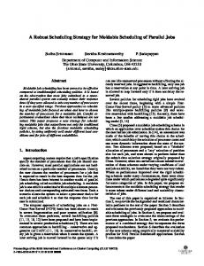
Figure 1: Structure and operation of the proposed crossdocking model

for augmenting the algorithm to a re-starting heuristic to construct a number of feasible trailer sequences for optimization purposes is also discussed and experimented. Finally, Section 6 concludes the paper and highlights our future research directions. 2. Crossdocking Model Development Figure 1 presents the proposed crossdocking model where a number of trailers are crossdocked in a multiple door crossdock. Trailers are assigned to dock doors on a daily basis to exchange some of their products before being dispatched to their customers. (The exchange pattern is known in advance.) Products are staged onto staging areas until their destination trailers are docked in the crossdock. Without loss of generality, we assume that the products whose destination trailers have not yet been assigned to an available door are temporarily staged in front of the doors that have been assigned their source trailers. The formation of staging areas is illustrated in Figure 1, based on Bartholdi and Gue’s observation from real crossdocks [21]. As the figure shows, some space is reserved in front of each door to stage freight for that door. In this study, we employ synchronous crossdocking which requires that all the trailers be available in the crossdock yard before the crossdocking operation starts. Truck scheduling starts when the first trailer is assigned to a door and ends when the last trailer leaves its assigned door. As soon as a trailer is assigned to a free door, a worker unloads the exchanged products onto the staging area provided in front of the door. The products are then moved by forklifts and discharged onto the respective staging areas of the doors to 4

which their destination trailers are assigned. Similar to unloading, a worker is dedicated for loading the exchanged products onto a destination trailer. Simply put, what is done inside the crossdock is to unload, move, and load the exchanged products between the trailers. 2.1. Truck Scheduling Formulation To formulate the truck scheduling problem addressed in this paper, it is required to sketch how products are exchanged among trailers in the crossdock. This is explained by applying the following operational characteristics to the crossdocking model: • Products are packed in pallets where all the products in an exchanged pallet are destined to one destination trailer. • The unloading operations of a trailer can be initiated as soon as it is assigned to a dock door. • The loading operations of a trailer can start only after its unloading operations are completed. • A trailer is ready to release its assigned door and leaves the crossdock when its loading operations are completed. • Trailer changeover time is the same for all trailers. • Pallets are unloaded or loaded by a worker one at a time. Also, only one worker can unload/load pallets from/onto a given trailer at any time. • A worker unloads or loads a pallet in one time unit. • Pallets are unloaded in sequence according to the order they have been placed at the supplier side and loaded according to the order they arrive at the destination door. (The former is input to the problem while the latter is determined during the crossdocking operation.) • A forklift can move only one pallet per trip. • A forklift moves a pallet (from its origin door) to its destination door only if the recipient trailer has been assigned to that door. • The velocity of a forklift is assumed to be one meter per second, making moving time and moving distance interchangeable. • The distance between any two doors is equal to the distance between their respective staging areas. 5

• Pallets are moved in rectilinear paths due to the aisles created by staged freight (see [22]). • The space allocated in front of each door does not overflow as a result of staged freight. The functionality of the aforementioned crossdocking operations is subject to the availability of the crossdock resources including dock doors, forklifts and workers, which are considered limited. The number of trucks in the crossdock yard may exceed the number of doors, leading to queues of trucks waiting to be assigned to doors. (In this study, we define the ratio of the number of trucks to the number of doors as the trailer-to-door ratio and denote it by α.) Likewise, there might be delays in pallet handling time due to the unavailability of workers and forklifts. If no worker is available, a delay should be incurred into the pallet unloading/loading time till one worker is available. Normally, these workers are the truck drivers themselves [23], allowing the delays to be negligible. In terms of forklifts, however, the amount of delays depends on the total number of forklifts operating in the crossdock and how they are scheduled for the service. If we assume one forklift is dedicated to each door for moving its unloaded products, respectively, then the forklift scheduling problem is reduced to the problem of scheduling the movements of each single forklift based on the scheduling conditions of only those trailers which are waiting to receive the unloaded pallets. A procedure can be embedded into the truck scheduling algorithm (see Section 3.2) to construct the moving order of the pallets unloaded in front of each door to their respective destination doors. Having known the orders, the delays can be calculated in a straightforward way on the proviso that no freight congestion nor interference among forklifts occurs to vary the forklift velocity. For example, for two pallets (unloaded at the same door) where the first one precedes the other in the moving order list, the latter should wait until the corresponding forklift moves the former to its destination door and then returns to the origin door. When the number of forklifts is fewer than the number of doors, the delays can be bounded by integrating a more complex forklift scheduling problem into the current problem. This is, however, beyond the scope of this paper so we assume the number of forklifts is equal to the number of doors. The allocation of doors, forklifts and workers is considered non-preemptive. In terms of doors, this means that a trailer does not release its assigned door unless it completes its operations (i.e., unloading/loading). Regarding forklifts and workers, they cannot be interrupted for another service until they finish moving and unloading/loading their assigned pallet, respectively. Non-preemptive door assignment makes it necessary to investigate the feasibility of the truck scheduling problem before its optimality as the problem might be entrapped in deadlock and no feasible solution is produced. Accordingly, the truck scheduling problem studied in this paper is formulated as the problem of constructing a feasible sequence of trailers for the assignment to dock doors and assigning each sequenced trailer to a proper dock door, 6

subject to a limited number of forklifts equal to the total number of doors, such that significant savings in the total crossdocking operation time (starts when the first trailer is assigned to a door till the last trailer leaves its assigned door) are achieved. The objective function, i.e., schedule length, is also referred to as makespan. 2.2. Integer Program The truck scheduling problem studied in this paper can be represented analytically in the context of an integer program. In the mixed integer programming (MIP) formulation, |J| trailers are waiting for crossdocking in a crossdock of |M | doors. The location of the crossdock doors is represented by their respective distances. There are in total |P | pallets exchanged between the trailers. For any two trailers which exchange some of their products with each other, a pallet unloaded from one of them is loaded onto the other. Accordingly, each trailer j has two sets of pallets. The first set contains those pallet IDs unloaded from the trailer2 (denoted by Uj ) and the second contains those loaded onto the trailer (denoted by Lj ). The following notation is used to describe the MIP model:

m

Indices door, m ∈ M = {1, . . . , |M |}

j p

trailer, j ∈ J = {1, . . . , |J|} pallet, p ∈ P = {1, . . . , |P |}

dmm′

Input parameters distance between doors m and m′

Uj Lj

set of pallets unloaded from trailer j set of pallets loaded onto trailer j

βp

unloading position of pallet p

C

T Q

trailer changeover time a big number representing maximal completion time difference between any two crossdocking operations

Cmax

Decision variables schedule length (or makespan)

aj cj

assignment time of trailer j completion time of trailer j

λp µp

time when moving of pallet p starts time when moving of pallet p is completed

σp

time when loading of pallet p is completed

δ γpp′

1, if for pallets p and p′ staged onto the same staging area, p is moved before p′ , else 0 1, if for pallets p and p′ loaded onto the same trailer, p is loaded before p′ , else 0

xjm yjj ′

1, if trailer j is assigned to door m, else 0 1, if for trailers j and j ′ assigned to the same door, j precedes j ′ , else 0

pp′

2

For a given n entities, entity IDs simply range from 1 to n.

7

vjmj ′ m′

product elimination variable to replace the nonlinear term xjm · xj ′ m′

With the above denotations and decision variables, the MIP formulation is as follows: Minimize s.t.

Cmax

X

xmj = 1, j ∈ J

(1)

m∈M

aj ′ ≥ cj + T C − Q · (1 − yjj ′ ), j, j ′ ∈ J, j 6= j ′

(2)

λp ≥ aj + βp , p ∈ Uj , j ∈ J

(3)

λp ≥ aj , p ∈ Lj , j ∈ J

(4) ′

′

′

′

λp′ ≥ λp + 2 · dmm′ · vjmj ′ m′ − Q · (1 − δpp′ ), p ∈ Uj ∩ Lj ′ , p ∈ P, p 6= p , j, j ∈ J, m, m ∈ M

(5)

µp ≥ λp + dmm′ · vjmj ′ m′ , p ∈ Uj ∩ Lj ′ , j, j ′ ∈ J, m, m′ ∈ M

(6)

σp ≥ µp + 1, p ∈ P

(7)

σp ≥ aj + maxp′ ∈Uj βp′ + 1, p ∈ Lj , j ∈ J ′

′

(8)

σp′ ≥ σp + 1 − Q · (1 − γpp′ ), p, p ∈ Lj , p 6= p , j ∈ J

(9)

cj ≥ σp , p ∈ Lj , j ∈ J

(10)

Cmax ≥ cj , j ∈ J

(11)

Constraint (1) ensures that each trailer is assigned exactly to one door. Constraint (2) defines the timing dependencies between two different trailers that have been assigned to the same door. It states that the assignment time of a trailer to a door is after the completion time of the other (which precedes the former trailer in being assigned to the same door) plus the time it takes to leave the door, i.e., the trailer changeover time. Having been assigned to a door, a trailer can start and complete unloading pallets consecutively according to the position they have been placed at the supplier side. Constraints (3)–(5) specify the conditions required to be met before an unloaded pallet can be moved. Constraints (3) and (4) state that the movement of a pallet cannot be started unless it is unloaded and its destination trailer is assigned to an available door. Constraint (5) schedules the movement of the unloaded pallets staged in front of a door according to the order which itself is decided during the scheduling. Note that Constraint (5) implicitly emulates the situation where exactly one forklift is designated to one door for moving its staged pallets. For two pallets where the first one precedes the other in the moving order list, the latter should wait until the corresponding forklift moves the former to its destination door and then returns to the origin door. Constraint (6) determines when the moving operation of a given pallet is completed. Constraint (7) ensures that a pallet is loaded only after it is moved to its destination door. Constraint (8) indicates that a trailer can start its loading operations only after it completes its unloading operations. Constraint (9) 8

states that the loading operations of the pallets onto a given trailer are completed consecutively according to the order they arrive at the destination door. Constraint (10) specifies that after loading its last pallet, a trailer is done and is ready to leave its assigned door. Constraint (11) defines the makespan which is equal to the maximum completion time of the trailers. Finally, the binary variables yjj ′ , δpp′ , γpp′ , and vjmj ′ m′ which have been used as control variables in the main constraints are defined by Constraint (12), Constraints(13), Constraints(14–15), and Constraints(16– 18), respectively: X

vjmj ′ m , j, j ′ ∈ J, j 6= j ′

(12)

vjmj ′ m , p ∈ Uj , p′ ∈ Uj ′ , p 6= p′ , j, j ′ ∈ J

(13)

yjj ′ + yj ′ j =

m∈M

δpp′ + δp′ p =

X

m∈M

γpp′ ≥ (µp′ − µp )/Q, p, p′ ∈ Lj , p 6= p′ , j ∈ J

(14)

γpp′ ≤ 1 + (µp′ − µp )/Q, p, p′ ∈ Lj , p 6= p′ , j ∈ J

(15)

vjmj ′ m′ ≤ xjm , j, j ′ ∈ J, m, m′ ∈ M

(16)

vjmj ′ m′ ≤ xj ′ m′ , j, j ′ ∈ J, m, m′ ∈ M

(17)

vjmj ′ m′ ≥ xjm + xj ′ m′ − 1, j, j ′ ∈ J, m, m′ ∈ M

(18)

In this formulation, the input parameter Q is a very big number greater than the completion time difference between any two crossdocking operations and is calculated as follows: Q = 2 · |P | +

X

m∈M

X

dmm′ + |J| · T C

m′ ∈M

It is observed that the MIP model indeed solves three decision sub-problems embedded in the truck scheduling problem addressed in this paper: 1. To which door should trailers be assigned? (represented by decision variable xjm ) 2. How to sequence the queue of waiting trailers assigned to the same door? (represented by decision variable yjj ′ ) 3. How to schedule the movement of pallets to their destination doors when one forklift is available at each origin door? (represented by decision variable δpp′ ) The above statement implies that by knowing the values of xjm , yjj ′ , and δpp′ , the values of the remaining decision variables are also known and the problem will be solved. It is worth noting that in the proposed two-phase heuristic algorithm, the values of the above three decision variables are determined in 9

the second phase after a feasible sequence of trailers (with respect to a given number of doors) has been constructed in the first phase.

3. A Two-Phase Heuristic Algorithm As it will be noticed in Section 5.1, the mathematical model developed in the previous section is inefficient, or even impractical, for solving real size problem instances. Having the same operational characteristics assumed in the development of the MIP model, we thus propose a two-phase heuristic algorithm to solve the truck scheduling problem. In the first phase, called truck sequencing, a dependency ranking search (DRS) heuristic is developed that, with a given number of doors, exhaustively searches the solution space until it finds a feasible trailer sequence. The search path is dynamically adapted by ranking trailers according to their dependency relationships. In the second phase, called door assignment, trailers are assigned to doors according to the sequence list generated in the first phase. This is done by developing a door fitness (DF) heuristic that deploys a fitness mechanism to choose and assign a proper door to a given trailer. The DF heuristic also schedules the movement of the forklifts operating in the crossdock. 3.1. Sequencing Phase: DRS Heuristic Non-preemptive door assignment adopted in the truck scheduling problem incurs complexities in its solution feasibility when the number of trailers is more than the number of doors (i.e., α > 1). The reason is that the problem might be entrapped in deadlock. The situation was first observed in our previous work [20] where we proposed a dependency ranking (DR) constructive heuristic for a similar truck scheduling problem. The infeasibility occurs because the heuristic is not robust in detecting and avoiding deadlock while constructing the sequence of trailers for the assignment to dock doors. (The DR heuristic will be reused in this paper for evaluation purposes.) Accordingly, this section aims at developing a robust heuristic search algorithm to address the issue of deadlock. The following example better illustrates our motivation to develop the DRS algorithm: Example. Consider the problem of scheduling eight trailers appointed to exchange some of their products in a four-door crossdock. The product exchange matrix is given by Figure 2(a). (Note that the matrix is the input to the problem.) In this figure, the row to each trailer indicates the number of products unloaded from that trailer while the column shows the number of products loaded onto the trailer. The trailers receiving products from a given trailer are called the successors of the trailer and those giving products are the predecessors of that trailer. The successors and predecessors of a trailer form the dependency relationships, or more concisely, the interdependencies, of the trailer. The truck scheduling feasibility depends on the interdependencies of trailers and not the number of products they exchange. Alternatively, a directed graph (DG) in which nodes are trailers and directed edges are their interdependencies is more representative than an exchange matrix. Figure 2(b) depicts the corresponding directed graph for the example in Figure 2(a).

10

Figure 2: (a) Product exchange matrix of eight trailers (the row to each trailer indicates the number of products unloaded from that trailer while the column shows the number of products loaded onto the trailer), (b) the interdependency DG, and (c) the spanning tree formed by Tarjan’s SCC algorithm

One strategy to schedule the trailers is to decompose the interdependency DG into its strongly connected components (SCC), e.g., by Tarjan’s algorithm [24], and schedule each SCC according to the order its vertices are reached, i.e., while its corresponding subtree is being formed. For this example, the given interdependency DG is already strongly connected so a spanning tree would be generated. Figure 2(c) shows the spanning tree from which the following trailer sequence is formed: 1 → 5 → 3 → 2 → 7 → 8 → 6 → 4. Now if the trailers are assigned to the doors according to the above order, at the time of assigning trailer 7 no free door is available and the scheduling process is forced to stop. This is because all the four doors have been assigned trailers 1, 5, 3, and 2, respectively, and cannot be released. Trailer 1 cannot complete its operations (and thus cannot free its assigned door) unless trailers 6, 7, and 8 are assigned to a door and unload its required products. A similar situation applies to trailers 5, 3, and 2 which have been assigned to the remaining three doors. (The only trailer that could complete its operations and leaves the crossdock is trailer 4 which is scheduled after the assignment of trailer 3.) This situation is referred to as deadlock. It occurs because door preemption is not allowed throughout scheduling. The same condition applies if the DR heuristic is used to schedule the trucks (see [20]). Given the sequence 8 → 1 → 7 → 2 → 3 → 4 → 5 → 6 generated by the DR algorithm, trailer 5 cannot be scheduled due to the deadlock caused after the assignment of trailers 1, 7, 3, and 4 to the four doors of the crossdock. On the other hand, if the trailers are scheduled according to the sequence 8 → 7 → 1 → 2 → 6 → 5 → 4 → 3, deadlock does not occur and a feasible solution will be produced.

The above example underlines the importance of developing a solution technique that is capable of avoiding, or detecting and resolving deadlock3 . Suppose either of the suggested strategies (Tarjan or the DR algorithm) is implemented in an industrial setting. Both approaches oblige the terminal manager to allocate at least five doors to schedule the eight trailer whereas a feasible schedule does exist for only four doors. It may be, however, so costly, or even impossible from a practical viewpoint to open an extra door to crossdock the trailers. 3

For some truck scheduling problem instances, deadlock occurrence is inevitable with respect to a particular number of doors. In that case, the truck scheduling problem is infeasible [for that number of doors].

11

The proposed DRS heuristic benefits from three main features to establish a feasible solution for the truck scheduling problem. First, the algorithm incorporates the number of available doors into its sequencing procedure to ensure feasibility throughout the search. Second is the ranking methodology that attempts to avoid deadlock by maintaining door availability each time a trailer is sequenced. The strategy is to expedite the sequencing process of the trailers which contribute products to more trailers. Finally, the third feature is backtracking which enables the algorithm to recover from deadlock (whenever entrapped) by retrieving its previous state and adjust its search path. DRS localizes its sequencing process by starting from a subset of tightly interdependent trailers and gradually moving to other interdependent subsets until all trailers are sequenced. Localization is performed by defining clusters. Each trailer together with its successors and predecessors form a cluster. This implies that the number of clusters is equal to the number of trailers where each cluster ID is represented by the ID of the corresponding trailer. Given the parameters defined in Table 1, the cluster Ci corresponding to trailer i is formed as follows: Ci = {i} ∪ Si ∪ (Pi \ R), i ∈ /R

(19)

Note that trailers having no predecessors are sequenced pre-maturely (as they are not dependent on other trailers and can release their assigned door on their own) and are not involved in the formation of clusters. Two ranking criteria are defined to choose the initial cluster. The first is based on how well the cluster members can internally contribute to each other and referred to as the internal rank. The next criterion is based on the contribution of the cluster members to the external trailers and is called the external rank. The internal and external ranks riI and riE of cluster Ci are calculated according to the following two Table 1: Parameters defined to describe the DRS algorithm parameter Si Pi Ci riI riE L A R cL i cA i ri

description successors of trailer i predecessors of trailer i cluster corresponding to trailer i internal rank of cluster i external rank of cluster i candidate list of trailers for sequencing and assignment trailers assigned yet have not released their assigned door trailers that have released their assigned door contribution of trailer i when it is included in L contribution of trailer i when it is included in A rank of trailer i in the candidate list L

12

formulas, respectively: riI =

|Pj ∩Ci | j∈Ci |Pj \R|

P

|Ci | riE =

P

j∈Ci

+

X

j

|Pj ∩Ci | |Pj \R|

|Ci | − 1

|Sj \ Ci |

k

−1

(20) (21)

j∈Ci

Note that the second term of Eq. (20) considers an additional bonus if all the predecessors of any cluster member (excluding the corresponding trailer – see ‘−1’) are in the cluster as well. The initial cluster is the one having the highest internal rank. In case of ties, the cluster with the highest external rank is chosen. When the initial cluster is identified, its members are included in a list called the candidate list. The candidate list holds a group of tightly interdependent trailers from which one trailer is sequenced in each iteration. Similar to clusters, each trailer in the candidate list is ranked and the one with the highest rank is chosen for sequencing. The methodology to rank a trailer in the list is made up of a number of elements. The first element represents the contribution of the trailer to the other trailers in the candidate list and those that have been sequenced (and assigned), yet have not released their assigned door. The contribution cL i of trailer i in list L is described analytically as follows: cL i =

|Si ∩ L| + |Si ∩ A| |Pi \ (A ∪ R)|

(22)

The contribution of these other trailers themselves is accounted as the second element of the proposed ranking mechanism. The trailers are either in the candidate list or have been sequenced and assigned to a door. For the former case, the contribution is calculated similarly according to Eq. (22). For the latter, the contribution of a trailer also applies to the trailers that neither have been sequenced and assigned to a door nor included in the candidate list. The following formula computes the contribution cA i of trailer i in set A: cA i =

|Si \ R| |Pi \ (A ∪ R)|

(23)

The third element indicates how tight is the trailer interdependent on the other trailers in the candidate list. This is specified by knowing how many trailers in the list are both the successors and predecessors of the trailer. The last element gives an additional bonus to the rank of the trailer if it serves as a predecessor of any assigned trailers that have not yet released their assigned door. The next formula integrates the

13

above four elements to calculate the rank ri of trailer i in list L: + j∈Si ∩A cA j ri = + + |Si ∩ L| + |Si ∩ A| X 1 |Si ∩ Pi ∩ L| + |Pi \ (A ∪ R)| j∈S ∩A |Pj \ (A ∪ R)| cL i

L j∈Si ∩L cj

P

P

(24)

i

Having sequenced and assigned the best trailer to a free door, the algorithm updates the candidate list by first deleting the trailer and second inserting its unsequenced predecessors, if any. It then monitors the allocation status of the doors. Two situations may occur. One is that the assignment of the trailer has maintained, or even improved, door availability. The other is that door availability is no longer maintained. In the latter case, DRS is entrapped in deadlock and, as explained in the next paragraph, requires backtracking to resolve it. In the former case, the algorithm searches for any trailer that can be released. A trailer is released if all of its initial predecessors have been sequenced and assigned to a door (whether or not these trailers themselves have freed their assigned door). Depending on the status of a ready-to-release trailer, DRS does one of the following two actions. If the trailer is already assigned, the algorithm simply frees the assigned door; otherwise, it will directly sequence the trailer by inserting it to the trailer sequence list. The above steps continue until no trailers can be released. The algorithm then ranks the current trailers in the candidate list to find and sequence the next best trailer for the next iteration. The sequencing procedure continues until the candidate list becomes empty. In case the candidate list is empty but there are some trailers still unsequenced, it means that there is at least one subset of trailers having no or loose interdependencies with those already-sequenced ones. In that case, DRS resumes its sequencing procedure by ranking the clusters corresponding to the remaining trailers and reinitializing the candidate list. The above courses of action repeat until all trailers are sequenced. As stated in the preceding paragraph, it is possible that, after a trailer is sequenced and assigned to a free door, no door is left available and no assigned trailer can be released. In that case, the sequencing process is not straightforward and encounters deadlock. DRS is equipped with backtracking to resolve deadlock. By backtracking, the algorithm goes one level back and chooses the next best trailer from the candidate list based on the ranking and selection criteria already introduced. If no more trailer is left untried, backtracking takes the sequencing status one further level back. In a situation where backtracking has reached the first level and all the trailers of the initial cluster have been examined yet no feasible solution is available, DRS performs re-starting by choosing the next best cluster and resumes the sequencing process. This continues until a feasible solution is found or all possible sequence patterns are tried by re-starting from the remaining clusters. In other words, the algorithm exhaustively searches the entire solution space 14

to find a feasible trailer sequence. If no solution is found, it is guaranteed that deadlock occurrence is inevitable with respect to the given number of doors. (The above maxim can be proved by a simple counter example.) Algorithm 1 describes the DRS heuristic in pseudo codes: Algorithm 1 DRS Heuristic 1. 2. 3. 4. 5. 6. 7. 8. 9. 10. 11. 12. 13. 14. 15. 16. 17. 18. 19. 20. 21. 22. 23. 24. 25. 26. 27. 28. 29. 30. 31. 32. 33. 34. 35. 36. 37. 38.

Sequence any trailer i whose Pi \ R = ∅; Form and rank Ci for each unsequenced trailer i; for all i where Ci has not been tried yet do if no cluster is found then Stop; {no feasible solution is found} else Choose the cluster with the highest rank; end if end for Initialize L with the trailers of the best cluster; while L 6= ∅ do Rank the trailers in L; for all i ∈ L where trailer i has not been tried yet do if no trailer is found and sequencing is in Level 1 then goto Line 3; {re-start from the next best cluster} else if no trailer is found then Retrieve the previous level; {backtrack occurs} goto Line 13; else Sequence the trailer with the highest rank; Remove the trailer from L and add it to A; Add its unsequenced predecessors to L; Check for door availability; if door availability is not maintained then Retrieve the previous level; {backtrack occurs} goto Line 13; else Search for any trailer that can be released; Update L, A, and R accordingly; end if end if end for end while if any unsequenced trailer is left then goto Line 2; else {a feasible solution is found} return the sequence list; end if

The efficiency of the DRS algorithm in establishing solution feasibility is evaluated against the DR heuristic. In the DR sequencing procedure proposed in [20], each trailer is ranked according to the ratio of the number of its successors to the number of its predecessors. Given the parameters defined in Table 2, the rank ri of trailer i is analytically described as follows: ri =

|Si | |Pi \ S|

15

(25)

parameter Si Pi S ri M

Table 2: Parameters defined to describe the DR algorithm description successors of trailer i predecessors of trailer i list of sequenced trailers rank of unsequenced trailer i unsequenced trailers whose ranks have changed since the first iteration

The trailer with the highest rank along with its predecessors are sequenced afterwards. The sequenced trailers are removed from the lists of unsequenced trailers and their unsequenced predecessors, respectively. The remaining unsequenced trailers are ranked again so that the next trailer with the highest rank together with its (unsequenced) predecessors are sequenced. The above steps repeat until all trailers are sequenced. As the DR algorithm does not verify the feasibility of the generated sequence list against a certain number of doors, solution feasibility cannot be ensured. We thus propose two other variations of the algorithm on the quest for reducing deadlock probability. In the first variation, rather than repeatedly sequencing a trailer and its predecessors, after sequencing one trailer, the algorithm searches for any unsequenced trailer whose rank is infinity, i.e., the number of its unsequenced predecessors is zero. If any trailer is found, it is sequenced immediately. The second variation, while including the previous amendment, localizes the sequencing procedure. After the best trailer and its predecessors are sequenced in the first iteration, the selection mechanism finds the next best trailers – for the remaining iterations – among those unsequenced trailers whose ranks have changed until then. Algorithm 2 describes the three versions of DR in one place in pseudo codes: Algorithm 2 DR123 Heuristic 1. 2. 3. 4. 5. 6. 7. 8. 9. 10. 11. 12. 13. 14. 15. 16. 17.

M ← ∅; {M has no member initially} Rank all the trailers; while any unsequenced trailer is left do if M 6= ∅ then Sequence the trailer i ∈ M with the highest rank; else Sequence the trailer i with the highest rank; end if Sequence any trailer j where Pj \ S = ∅; {versions 2 & 3} while Pi \ S 6= ∅ do Sequence one unsequenced predecessor of trailer i; Sequence any trailer j where Pj \ S = ∅; {versions 2 & 3} end while Repeat ranking the remaining unsequenced trailers; Update M ; {version 3} end while return S;

The three versions of DR form a so-called DRb heuristic whose solution output is defined as the minimum of the three solutions and runtime as the sum of the three running times. Note that irrespective of which algorithm is deployed (i.e. DRS or any variation of DR), a trailer sequence list will be generated 16

as the output. The sequence list is then given to the DF assignment algorithm to produce the final solution which is the makespan. 3.2. Assignment Phase: DF Heuristic The DF heuristic follows a greedy approach to choose a proper door for each trailer picked from the sequence list. The selection mechanism is developed by defining a fitness for each door. The door attaining the best fitness is then chosen and assigned the trailer. The most apparent criterion to characterize the fitness of a door is its availability time. A door having an earlier availability time is a better candidate for the assignment. To realize whether the interdependencies of the given trailer should also be considered by the selection mechanism or not, we divide them into two categories. One includes those successors and predecessors of the trailer whose position in the sequence list is before the trailer and the other includes those whose position is after. The assignment information of the trailers in the former category, including the assignment time and assigned door, is known at the time of assigning the given trailer itself whereas for the trailers in the latter category, no exact information is available and estimation should be used. In our preliminary experimentations, however, we observed that estimated information does not help to improve the solution quality but rather severely worsens the final results. This is due to the high complexity of the problem which makes the estimation procedure complicated, and hence, inaccurate. On the contrary, including the exact assignment information (of the trailers in the former category) in the fitness function did help to improve the makespan. For the cases where no exact assignment information is available about any of the successors or predecessors of the trailer (e.g., when the first trailer in the sequence list is to be assigned), the physical location of the doors in the crossdock is included in the fitness function. The physical location of a door is assessed by its average (rectilinear) distance to all other doors on the dock [21]. Given the parameters defined in Table 3, the physical location li of door i is calculated as follows: li =

P

j∈D\{i} dij

(26)

|D| − 1

To calculate the fitness of a door relative to a given trailer, we sum the availability time of the door and the cumulative travel times of the pallets exchanged between the trailer and those of its successors and predecessors whose assigned door is known at the time of assigning the trailer itself. The fitness fi′ of door i′ , candidate for the assignment of trailer i, is computed according to the following formula: f i′ = t i′ +

X

j∈Si

nij · di′ j ′ +

∩T D

X

j∈Pi

17

∩T D

nji · dj ′ i′

(27)

Table 3: Parameters defined to describe the DF algorithm parameter D ti dij li Si Pi TD i′ nij ei fi

description doors of the crossdock availability time of door i (rectilinear) distance from door i to door j physical location of door i successors of trailer i predecessors of trailer i trailers whose assigned door is known (candidate) assigned door i′ of trailer i number of pallets sent from trailer i to trailer j total number of exchanged pallets of trailer i fitness of door i (measured in time)

In case no exact assignment information is available, the value representing the physical location of the door is multiplied by the total exchanged pallets of the trailer. The product (which is measured in time because distance and time are interchangeable) is added to the availability time of the door to form its fitness. The following formula analytically describes how the fitness fi′ of door i′ , candidate for the assignment of trailer i, is calculated in that case: fi′ = ti′ + ei · li′

(28)

The door acquiring the smallest value scores the best fitness and is chosen for the assignment of the trailer. Note that Eq. (27) is invoked only if the assigned door of at least one of the trailer’s successors or predecessors is known; otherwise, Eq. (28) is used for computing the fitness. Also note that at the time a trailer is assigned, the fitness construction includes only those doors whose availability time is known. The availability time of a door can be measured only if the release time of its latest assigned trailer is known. The release time of a trailer depends on the location of the doors to which the predecessors of the trailer are assigned. Consequently, if no exact information is available about the assigned door of at least one of the predecessors, it is not possible to calculate the trailer’s release time, and hence, the availability time of its assigned door. Finally, it should be explained why forklift availability times are not included in the computation of the fitness function. The reason is that the fitness of a door, for a given trailer, does not depend on the availability time of the forklift dedicated to the door but rather depends on the availability times of a number of forklifts that move the pallets loaded onto the trailer from a number of origin doors. A direct inclusion of these values in the fitness function would bias the fitness from its main element which is the door availability time. On the other hand, an indirect inclusion demands a more complicated and exhaustive analysis beyond the scope of this paper. Having assigned the trailer to the door, we require to schedule the movement of pallets both unloaded

18

from the trailer and those loaded onto the trailer. For the latter, the scheduling is straightforward. According to the order it is unloaded, each pallet is moved by the forklift dedicated to its origin door. For the former, the situation is different as all the pallets4 must be moved by only one forklift. Since the pallets might have different destinations, we need a scheduling policy to order their movements. Our strategy is to prioritize the movement of the pallets according to the completion status of their recipient trailers. The completion status of a trailer is assessed by the latest position that one of its predecessors holds in the sequence list. The recipient trailers are then sorted in ascending order of their completion status. This means that a trailer having a smaller value receives its required pallets earlier than another with a larger value. The smallest possible value belongs to one (or more) recipient trailer(s) whose last predecessor is the currently assigned trailer. Accordingly, as soon as the trailer receives its required pallets, it can complete its final loading operations and releases its assigned door. It is expected that the proposed scheduling policy shortens the completion time of the trailers, and hence, reduces the makespan. A similar expectation is also desired for the algorithm’s fitness function. Algorithm 3 describes the DF heuristic in pseudo codes: Algorithm 3 DF Heuristic 1. while sequence list 6= ∅ do 2. Pick the current trailer from the sequence list; 3. for all i where door i is available do 4. if no available door is found then 5. Stop; {deadlock occurs} 6. else 7. Calculate the fitness of the available doors; 8. Assign the trailer to the door with the best fitness; 9. Schedule the forklifts that move the exchanged pallets; 10. Update timings of the docking activities involved; 11. end if 12. end for 13. end while 14. return the makespan;

4. Test Data Generation There is no real data available to evaluate the performance of the proposed heuristic algorithms. Alternatively, we generate synthetic data according to the methodology introduced by Shakeri et. al [25] for the same truck scheduling problem. Each category of the test data characterizes four elements: the size of the crossdocking terminal (formally represented by the number of doors [21]), queue length of waiting trailers (i.e., the value of the trailer-to-door ratio), product exchange patterns between trailers, and correlation 4

This includes only those pallets which are ready to be moved. That is, their recipient trailers have already been assigned to a door.

19

status of interdependent trailers. The values assumed for the number of doors and trucks are summarized in Table 4(a). The table defines four data sizes from small to huge with four different values of the trailer-to-door ratio for each size. The patterns for the exchange composition of a trailer are formalized by three freight mixed levels (FMLs) defined in Table 4(b). A freight mixed level is quantified by the percentage of the trailers receiving the exchange volume of each single trailer. This also specifies the level of interdependencies defined between trailers. All trailers have a maximum capacity of 60 products. The initial number of products in each trailer is uniformly distributed between 20 and 40 products. The amount of exchange for the trailers ranges evenly from half to all of its initial carrying products. For each trailer, a random number is generated uniformly in the interval corresponding to a particular mixed level to represent the number of trailers receiving the exchange volume of that trailer. Note that in the extreme case, the number of recipient trailers is equal to the number of exchanged products, i.e., each trailer receives one product. Lastly, to identify the IDs of the recipient trailers for each trailer, i.e., to form the interdependencies, two approaches are adopted: uncorrelated and correlated. In the uncorrelated approach, the IDs are chosen uniformly from the entire group of trailers while in the correlated one, the dependency history of the trailer, if any, is involved in the procedure of specifying the IDs. By the dependency history, we mean the list of the trailers which either have sent some products to the trailer or, together with the trailer, have received products from the same donor trailer. The correlated approach assigns higher probability to the trailers in the history list to be chosen as the recipient trailers. Since no clear data on the exact level of correlation are available in practice, a conservative correlation level is assumed to generate correlated test instances (see [25] for a concrete example). So, according to the steps introduced for the data characterization, each category of the test data is represented in a 3-tuple (size:α; FML; correlation status). In case one or more attributes are not reflected in the tuple, it means that the reduced tuple encompasses all the values of the missing attributes. For example, the tuple (small:1; low) represents both (small:1; low; uncorrelated) and (small:1; low; correlated) tuples. Finally, rectangular crossdocks are used for the experiments. Considering d the number of dock doors, d/8 doors are placed on the shorter side of the crossdock while 3d/8 are placed on the longer side. (Note that d is a multiple of 8.) The distance between doors is determined by assuming that the distance between adjacent doors (and between each corner and the closest door) is 1 distance unit.

20

Table 4: Test data characterization (a) Data sizes defined for the truck scheduling problem number number of trucks size of doors α = 1 α = 2 α = 4 α=8 small 8 8 16 32 64 medium 32 32 64 128 256 large 96 96 192 384 768 huge 256 256 512 1024 2048 (b) FMLs defined for the truck scheduling problem percentage (%) of trailers FML (that receive the exchange volume of each single trailer) low less than 10% of the total trailers medium 10% to 25% of the total trailers 5% to 50% of the total trailers with 95% probability high more than 50% of the total trailers with 5% probability

5. Experimental Results and Analysis The proposed heuristics are coded in C++ and run on a CoreTM 2 Quad 2.66GHz computer with 3GB RAM. To set up the experimental data, ten random instances are generated for each combination of the problem sizes, trailer-to-door ratios, freight mixed levels, and uncorrelated and correlated interdependencies (this equals to 4 × 4 × 3 × 2 × 10 = 960 total instances). At the first attempt, the MIP model described in Section 2.2 is compared with the heuristics in solving the truck scheduling problem. The model is implemented in the AIMMS modeling platform [26] and solved by the ILOG CPLEX 12.1. At the second attempt, the efficiency of the DRS algorithm in establishing solution feasibility is evaluated against the DRb sequencing heuristic. The evaluation metric adopted throughout the experiments is relative difference (r. d.). Given two algorithms A and B for the problem, the relative difference of B results from those of A is calculated according to the following formula:

r. d. (%) =

Cmax (B) − Cmax (A) × 100 Cmax (A)

(29)

Since the problem objective is to minimize the makespan, an improvement in the solution quality (obtained by a new algorithm, here B) is represented by a negative value of the relative difference. When the comparison of two (or more) solution techniques is based on average results, the mean function is applied to only those instances where all the compared solution techniques could produce a feasible solution. That is, if one algorithm finds a feasible solution for a given problem instance while the other fails, the value is not included in the mean function for the former algorithm. Finally, we adopt the following terminology to present the results in tables:

21

Bt: Number of backtracks invoked during the execution of DRS Rs: Number of re-starts invoked during the execution of DRS ST(s): Time (in seconds) taken for DRS to establish solution feasibility after the last re-starting, if any TT(s): Algorithm’s total runtime (in seconds) 5.1. Heuristics vs. Mathematical Model: Efficiency The efficiency of the MIP model in solving the truck scheduling problem is evaluated for small size instances. Given a time limit of two hours (a longer time limit for finding a feasible solution might not make sense for the real-time logistics of crossdocking), the CPLEX solver is able to find a feasible (but not optimal) solution only for 41 (out of 60) instances belonging to the (small:1) category. This is in fact the simplest form of the experimental data! The truck scheduling problem is to be solved in an eight-door crossdock where the number of trucks is equal to the number doors. The sequencing procedure of trucks is straightforward as exactly one door is available for each truck. The best results obtained by the proposed heuristic techniques (including DRS and the three variations of DR, combined with DF) are compared with those of the CPLEX solver. Table 5 presents the average results for the two approaches. To make a fair comparison, the running times of the four heuristic combinations are summed up and represented as the total runtime. As Table 5 indicates, heuristics exhibit much better performance in terms of both solution quality and runtime than the mathematical model for all the combinations of the freight mixed level and correlation status. We can conclude from the above observation that mathematical programming techniques are not efficient for solving this sort of detailed scheduling problems. The MIP model requires the solver to decide on the timing values and handling orders of every single pallet in the crossdock before producing the final solution, which is the overall schedule length. Although this flexibility in time gives total freedom to find the optimal solution, at the same time, it makes it very complicated for the solver to systematically branch and cut the search space as many intricate domain indices are defined in the model’s constraints (see Section 2.2). Table 5: Heuristics vs. mathematical model for (small:1) instances (average results are shown) FML low medium high

correlation status uncorrelated correlated uncorrelated correlated uncorrelated correlated

CPLEX2-hour Cmax 66.8 102 82.2 111.5 97.4 115.7

22

Heuristics Cmax TT(s) 40.7 0.21 41.1 0.17 45.3 0.24 44.6 0.17 45.2 0.22 50.5 0.19

r. d. (%) -39.07 -59.68 -44.83 -59.98 -53.59 -56.37

Table 6: DRS compared to DRb when FML is kept low and α is variable (average results are shown) data category (small:1) (small:2) (small:4) (small:8) (medium:1) (medium:2) (medium:4) (medium:8) (large:1) (large:2) (large:4) (large:8) (huge:1) (huge:2) (huge:4) (huge:8)

DRb +DF Cmax TT(s) 52.55 0.08 110.6 0.1 277.3 0.18 848.1 0.26 131.3 0.25 256.5 0.45 553.3 0.85 1591.2 1.72 428.5 1.25 716.4 2.46 1374.1 4.85 3515.9 9.7 1255.7 7.08 2055.9 14.1 3607.3 28.5 8731.7 57.5

Cmax 45.1 110.9 270.6 793.6 152.4 267.4 542.3 1342.4 487.2 735.3 1412.1 3087.6 1528.8 2295.6 3853.7 7881.5

DRS+DF TT(s) Bt 0.11 0 0.13 0 0.21 0 0.3 0.2 0.16 0 0.31 0 0.68 0 1.98 0 0.68 0 1.6 0 4.55 0 14.7 0 3.79 0 10.1 0 30 0 103 0

r. d. Rs 0 0 0 0 0 0 0 0 0 0 0 0 0 0 0 0

(%)

-14.2 0.27 -2.43 -6.43 16 4.25 -1.98 -15.6 13.7 2.64 2.76 -12.2 21.7 11.7 6.83 -9.74

5.2. DRS vs. DRb : the Trailer-to-Door Ratio DRS is compared with DRb by first varying the value of α and keeping FML low. This allows to merely investigate the complexity of the truck scheduling problem relative to the trailer-to-door ratio. The average results for the two solution approaches are shown in Table 6 (see [27] for the full coverage of the results). The table indicates that for the majority of instances representing large crossdocks with short queues of waiting trailers (the latter is specified by the value of α), DRb exhibits a better performance in solution quality than DRS – see the positive values of r. d. (%). The advantage is mainly due to the sequencing strategy of DRb which is based on the repeated sequencing of trailers and their predecessors. Consequently, it is more probable that the trailers are assigned to adjacent doors in the assignment phase, leading to more savings in pallet moving times and hence, the overall makespan (this is more significant for large crossdocks). On the other hand, as α increases and the problem becomes more complex, DRS performs better than DRb – see the negative values of r. d. (%). The reason should be sought in the DRS sequencing scheme. As inferred from Section 3.1, DRS aims at constructing a chain of sequenced trailers in which each trailer is highly interdependent on both its direct and indirect neighbors. Thus, irrespective of the number of total trailers, a neighborhood of tightly interdependent trailers can be found in any part of the sequence list that have been assigned to a number of adjacent doors in the crossdock. The accumulated savings gradually outweigh those of DRb as the value of α increases. An interesting observation is that both heuristic approaches maintain scalability in the runtime as the problem size increases to huge scales. For the extreme case of scheduling over 2000 trailers in a 256-door crossdock, the total runtime of the heuristics

23

does not exceed two minutes. 5.3. DRS vs. DRb : the Freight Mixed Level As mentioned earlier in Section 3.1, the studied truck scheduling problem might not have a feasible solution for the cases where α > 1. The experimentation conducted in the previous section, however, shows that establishing solution feasibility is not an issue when the freight mixed level is kept low, even for α = 8. Accordingly, the investigation on the problem feasibility should be carried out for more difficult instances of the higher mixed levels. The infeasibility of a problem with respect to a given data set can be proven either analytically or experimentally by exploring the entire solution space. The latter approach applies to our case as we can make use of the DRS algorithm, which is inherently an exhaustive search technique5 , to decide on the problem feasibility. Since the solution space of the problem is exponentially increased by linearly increasing the number of trailers and doors, DRS is unable to search the entire solution space in a reasonable amount of time to confirm infeasibility. Alternatively, a miniature test case of scheduling 4, 8, 16, and 32 trucks in a four-door crossdock is generated using the methodology introduced in Section 4 to enable DRS to explore the whole solution space within moderate running times. For each combination of the trailer-to-door ratios, freight mixed levels, and uncorrelated and correlated interdependencies, i.e., 4 × 3 × 2 = 24 combinations, 200 random instances are generated and the number of feasible ones are recorded. Table 7(a) shows the percentage of the feasible solutions for each combination. The results indicate that the product of large trailer-to-door ratios and high freight mixed levels lead to infeasibility. The infeasibility region is formed by the combination of α = 8 and both the medium and high FMLs, and α = 4 and the high FML (represented in bold 0s in the same table). Note that feasibility is poor when α = 4 and FML is medium, and is not guaranteed when α = 2 and FML is high, and α = 8 and FML is low. It can be claimed that a similar allocation of feasible and infeasible regions, with comparable percentage, is applicable to larger size instances as first, the scaling is proportional and second, all data are generated according to an identical generation procedure. The above generalization is strongly supported by the results obtained by the DRS algorithm. To demonstrate how robust DRS is in avoiding deadlock and reaching feasibility with respect to larger size instances, the percentage of feasible solutions found by the DRS algorithm in a time limit of two hours is presented in Table 7(b). Due to space limitations, the table includes only the aggregate results from small to huge problem sizes for the six combinations of the trailer-to-door ratios, freight mixed levels, and uncorrelated and correlated interdependencies where 100% feasibility is not guaranteed. The consistency 5

DRS exhaustively explores the search space until it finds a feasible solution.

24

Table 7: Percentage (in %) of feasiblility for (a) Miniature instances (guaranteed by DRS) correlation over-constrained factor FML status α=1 α=2 α=4 α=8 uncorrelated 100 100 100 93.5 low correlated 100 100 100 98.5 uncorrelated 100 100 10 0 medium correlated 100 100 13 0 uncorrelated 100 92 0 0 high correlated 100 98 0 0 (b) Small to huge instances (found by DRb & DRS) over-constrained correlation FML DRb DRS factor status uncorrelated 97.5 100 low α=8 correlated 95 100 uncorrelated 0 5 medium α=4 correlated 0 15 uncorrelated 42.5 90 high α=2 correlated 57.5 100

in the robustness of the DRS algorithm is clearly affirmed by comparing the results of Tables 7(a) and 7(b). Table 7(b) also shows that DRS is more efficient than DRb in generating feasible solutions (there are totally 47 instances where DRb is not able to find a solution while DRS is – see [27] for more information). This implies that the combination of the ranking methodology and backtracking mechanism embedded in the DRS algorithm works well. It can be seen from Table 7 that the percentage of feasible solutions is slightly higher for correlated data instances. This is because correlation makes the interdependencies of the trailers more clustered so it is more probable to find a feasible solution based on a systematic scheduling of trailers in each cluster – as it is employed in the heuristics. The above observation also implies that for those real world case studies where the level of correlation in trailer interdependencies is higher than that considered in this work, the proposed DRS algorithm will perform efficiently in finding feasible solutions. 5.4. Discussion on DRS Efficiency The experimental results indicate that the DRS ranking methodology on its own cannot maintain a deadlock-free search path at all times and requires a backtracking mechanism to adjust it. In other words, the occasional failure of the methodology in avoiding deadlock is compensated by backtracking. The frequency of failures, however, varies from one occasion to another, implying that the ranking mechanism is dependent on the input data. The problem with recurring backtracks, as a result of frequent failures, is the huge overhead incurred on the algorithm runtime, impeding its capability to systematically find a feasible solution within a specified time limit, and hence, impairing its robustness. The following section introduces the mechanism deployed in the experiments to maintain a robust DRS and verifies its efficiency. 25

5.4.1. Robustness It was observed in the conducted preliminary experimentations that the choice of the initial cluster significantly affects the DRS performance to avoid deadlock and build a feasible solution. A poor initial cluster causes the algorithm to construct the trailer sequence list from an improper collection of trailers, leading to recurring entrapment in deadlock. As a consequence, a large number of backtracks are required to fix the constructed sequence list. In the worst case, no feasible sequence list could be found with respect to the given initial cluster and the algorithm must initiate a re-start to resume the sequencing procedure from a new initial cluster. To loosen the negative impact of a poor initial cluster, and hence, reduce the total runtime, the length of time where DRS is searching the solution space, after every selection of the initial cluster, is limited to a time when the number of backtracks is less than a certain limit. (The limit is varied from 1000 to 50000 backtracks in the experiments.) Whenever the solution time exceeds the assigned limit, the algorithm stops searching and initiates re-starting to choose the next best initial cluster according to the ranking and selection criteria defined earlier. The sequencing process is then resumed and the solution time is monitored again. This continues until a feasible sequence list is constructed, or the two hour time limit expires, or no more cluster is left to be selected as the initial cluster. The proposed amendment is quite effective. For all the data instances, where at least one re-start is required till a feasible sequence list is constructed, the solution time after the last re-starting, denoted by ST(s), is considerably smaller than the given time limit (see [27]). Although DRS proved to be robust in avoiding deadlock and generating feasible solutions, the imposed timing restrictions no longer ensure that the algorithm guarantees infeasibility in the case it does not find a feasible solution. For example, the average number of clusters examined by DRS within the assigned time limits is 24 and 12 for large and huge instances, respectively. This is considerably fewer than the potential number of initial clusters (which could be as many as 768 for large problems and 2048 for huge ones). As noticed in Section 5.3, finding a feasible solution is a bottleneck when α = 4 and FML is medium. In this data category, the number of initial clusters is 384 and 1024 for large and huge instances, respectively, implying that the DRS algorithm is able to check only 6.2% and 1.2% of their total number of clusters. This means that the algorithm robustness is heavily dependent on the ranking methodology developed in Section 3.1 for choosing the initial cluster. To evaluate the efficiency of the proposed cluster ranking methodology in choosing a good initial cluster, a purely random selection method was applied to uniformly choose the initial cluster among all the candidate ones for both large and huge instances where α = 4 and FML is medium. It is interesting to note 26

that at the first round, the random method even failed to produce a feasible solution for the three instances in the (large:4;medium;uncorrelated) and (large:4;medium;correlated) categories in the two hour time limit – this already confirms that the cluster ranking methodology is fairly efficient. Nevertheless, after the next nine rounds6 , the random approach was able to find a feasible solution within the two hour time limit for two more instances (where the rank-based method could not), one in the (large:4;medium,uncorrelated) category and the other in the (huge:4;medium,correlated). The DRS current robustness can be further improved by an intelligent randomization of the cluster selection step. The concept will be introduced as our future work in Section 6. 5.4.2. Solution Quality Not only does the initial cluster influence the robustness of the DRS algorithm in establishing solution feasibility, it also affects the quality of the final solution produced. An experimentation is conducted to evaluate how much improvement in the solution quality would be obtained if the initial cluster changes. The experimental data consist of those random instances where the relative difference of the DRS solution results from those of DRb exceeds 20% (totally 102 instances). The DRS+DF heuristics are then run ten times per instance where, each time, one cluster among the best ten clusters is selected as the initial cluster. (The first ten clusters acquiring the highest ranks form the best ten clusters.) Of the ten solutions generated, the smallest one, i.e., the best one, is recorded afterwards. The amount of improvement (i.e., minimization) for each random instance is scaled relative to the original value according to Eq. (29). The experimental results indicate that the amount of improvement is absolutely significant for most of the instances. Over -20% relative difference in solution quality has been obtained for nearly 70% (71 out of 102) of the test instances. The highest improvement is reported as -57.67% and the lowest is 0%. (The latter belongs to the (small:1) category where the number of initial clusters is at most eight.) The average improvement is equal to -26.46% (the total average is -29.46%) and the average deviation is 9.37%. The experimental results for 12 instances where the improvement exceeds -40% are shown in Table 8. The instances are sorted in descending order of their improvement. The table also presents some useful statistics on the results obtained from the whole 102 instances. By looking at the number of backtracks (Bt) required to adjust the search path for both the original and improved versions of DRS, it is inferred that choosing the best initial cluster has enabled the sequencing procedure to construct the feasible solutions systematically based on the ranking and selection criteria proposed. As the second last row of the table shows, the total number of backtracks for the entire 102 instances reduces from 73146 to only 5 times in 6

The random selection method was run for ten times.

27

Table 8: DRS efficiency in solution quality w.r.t. the initial cluster data category

#

(large:2;high;correlated) 6 (medium:1;medium;correlated) 9 (huge:1;low;uncorrelated) 9 (medium:1;low;uncorrelated) 3 (medium:2;high;correlated) 4 (small:1;medium;uncorrelated) 6 (large:1;high;correlated) 9 (huge:1;low;uncorrelated) 2 (small:1;low;correlated) 5 (large:4;low;uncorrelated) 10 (large:1;low;uncorrelated) 7 (huge:2;low;correlated) 10 sum (for the total 102 instances) average (for the total 102 instances)

DRb [+DF] Cmax 2309 182 1410 115 813 58 736 1067 41 1464 346 2124 93450 916.2

Original DRS[+DF] Cmax 4699 296 2154 203 1313 70 1356 1991 73 2018 622 3296 126714 1242.3

Bt 18 0 0 0 5 0 0 0 0 0 0 0 73146 –

Rs 0 0 0 0 0 0 0 0 0 0 0 0 – –

Improved DRS[+DF] Cmax 1989 143 1117 108 731 39 757 1117 41 1167 361 1942 89381 876.3

ST(s) 4.45 0.09 1.22 0.03 0.55 0.01 1.12 1.41 0 2.3 0.22 4.69 – 2.89

Bt 0 0 0 0 0 0 0 0 0 0 0 0 5 –

Rs 7 2 4 2 4 4 2 2 6 2 7 8 – –

DRS improvement r. d.(%) r.t. DRb Org. Imp. -57.67 103.5 -13.86 -51.69 62.64 -21.43 -48.14 52.77 -20.78 -46.8 76.52 -6.09 -44.33 61.5 -10.09 -44.29 20.69 -32.76 -44.17 84.24 2.85 -43.9 86.6 4.69 -43.84 78.05 0 -42.17 37.84 -20.29 -41.96 79.77 4.33 -41.08 55.18 -8.57 -29.46 35.59 -4.35 -29.46 35.59 -4.35

r. d.(%)

the case of constructing the sequence list from the best initial cluster. Note that the number of re-starts (Rs) in the Improved DRS[+DF] column of Table 8 can be used to identify which cluster has led to the best solution. For example, if the number of re-starts is zero it means the initial cluster is the first best cluster. If the number is 9 it means the initial cluster is the tenth best cluster and so on. As a comparison, the DRS+DF solution results, including the original and the improved ones, are evaluated against those of the DRb +DF heuristics. The last two columns of Table 8 indicate that the improved DRS outperforms DRb on average. (See the positive and negative values of relative difference – r. d. – for both the original and improved versions of DRS.) All of this implies that if DRS is augmented to a re-starting heuristic in which the solution construction is carried out iteratively from a number of clusters as the initial points, it is expected that much improvement would be attained in terms of deadlock avoidance (represented by the number of backtracks), solution quality, and runtime. 6. Concluding Remarks and Future Work This paper addressed the truck scheduling problem in a crossdocking terminal whose resources including doors, forklifts, and workers were assumed limited and non-preemptive. The crossdocking model, while having practical instances in the broad scope of the FMCG industry and military logistics, was purposefully specialized to visualize truck scheduling in the context of an integer program. Since non-preemptive door assignment incurs complexities in the problem feasibility, we developed an algorithmic approach capable of establishing solution feasibility for truck scheduling problem instances of various types and difficulty levels which at the same time can be readily implemented in an industrial setting. The proposed approach was a two-phase heuristic algorithm where, in the first phase, a dependency ranking search (DRS) heuristic was deployed to construct a feasible sequence of trucks for the assignment to dock doors and, in the second, a 28

rule-based heuristic was used to assign each sequenced truck to a proper dock door, subject to a limited number of forklifts equal to the total number of doors, such that significant savings in the truck schedule length could be achieved. Extensive experiments were conducted to evaluate the efficiency of the algorithm in terms of deadlock avoidance and solution quality. The evaluation was carried out against the solutions generated by the mixed integer programming (MIP) model of the problem and the three variations of a dependency ranking (DRb ) constructive heuristic developed in [20] for a similar truck scheduling problem. Experimental results demonstrated that the DRS algorithm is robust in avoiding deadlock and generates feasible solutions for the instances where the other two approaches cannot. Furthermore, the algorithm produced better solutions than DRb for more complicated problems where the ratio of the number of trucks to the number of doors is high. Given its accomplishments and limitations, the current work can be further improved from two perspectives: modeling and algorithmic. From the modeling point of view, the intermediate storage in the crossdock is not unlimited and should be represented by a number of limited staging areas distributed along the dock doors. Shakeri et. al [25] conducted an analysis to investigate whether the crossdock capacity is a bottleneck resource in the operation of truck scheduling or not. Having set up realistic values for the capacity of staging areas available in front of doors, the analysis showed that the entire crossdock capacity never overflows. Nonetheless, it was observed that the allocated space in front of doors might overrun the assigned limit. It is thus required to avoid space overrun while truck scheduling is in progress. An effective strategy is to concurrently monitor the number of products staged in front of each door. In case overrun occurs, a procedure is invoked to move the excess load to the appropriate locations where sufficient space is available. A post-processing procedure can also be used to balance the number of staged products in front of each door by utilizing forklift idle times. The utilization may even help to reduce the makespan by pre-moving pallets to their destination doors. From the algorithmic viewpoint, it was observed that DRS efficiency both in finding feasible and high-quality solutions is heavily dependent on the choice of the initial cluster. To further improve the robustness of the DRS algorithm in establishing solution feasibility, the current ranking heuristic rules can be supplemented by a few more ranking functions of different characteristics. An intelligent randomization function is then designed to choose the rules for ranking the clusters based on the status of the search. In other words, the selection of each ranking function is subject to a probability whose value is dynamically updated by the history of the search. This indicates that the choice of the initial cluster is adaptive (and not deterministic) to the input data. The important issue is how to define and adjust the ranking criteria of the functions such that they continually complement each other throughout the search. Moreover, as 29

demonstrated in Section 5.4.2, the re-starting helps to improve the solution quality. This can be extended to form a pool of good-quality feasible solutions of diverse attributes as the initial solutions of a neighborhood search method (such as a local search) to establish optimality. Acknowledgment This research is supported by the collaborative research project (CRP) between NTU and SIMTech and sponsored by NTU Graduate Scholarship. The authors would also like to thank Pim Beers, Senior AIMMS Specialist from Paragon Decision Technology Pte. Ltd. for his significant contributions in developing the mathematical model of the problem in AIMMS modeling language. References [1] Bozer YA, Carlo HJ. Optimizing inbound and outbound door assignments in less-than-truckload crossdocks. IIE Transactions 2008;40(11):1007–18. [2] Boysen N, Fliedner M, Scholl A. Scheduling inbound and outbound trucks at cross docking terminals. OR Spectrum 2010;32(1):135–61. [3] Cohen Y, Keren B. A simple heuristic for assigning doors to trailers in cross-docks. In: Int. Conf. Industrial Logistics (ICIL 2008): Logistics in a Flat World: Strategy, Management and Operations. Tel Aviv, Israel, Mar. 09-15; 2008, p. 1–14. [4] Gue K. Freight Terminal Layout and Operations. Ph.D. thesis; Georgia Institute of Technology; Atlanta, Georgia; 1995. [5] Li Z, Low MYH, Sim CH, Lim YG. Optimal product allocation for crossdocking and warehousing operations in FMCG supply chain. In: IEEE Int. Conf. Service Operations and Logistics, and Informatics, vols 1-2. Beijing, China, Oct. 12-15; 2008, p. 2963–8. [6] Li Z, Sim CH, He W, Chen CC. A solution for cross-docking operations planning, scheduling and coordination. In: IEEE Int. Conf. Service Operations and Logistics, and Informatics, vols 1-2. Beijing, China, Oct. 12-15; 2008, p. 2957–62. [7] Song K, Chen F. Scheduling cross docking logistics optimization problem with multiple inbound vehicles and one outbound vehicle. In: IEEE Int. Conf. Automation and Logistics, vols 1-6. Jinan, China, Aug. 18-21. ISBN 978-1-4244-1530-4; 2007, p. 3089–94. [8] Chen F, Lee CY. Minimizing the makespan in a two-machine cross-docking flow shop problem. European Journal of Operational Research 2009;193(1):59–72. [9] Chen F, Song K. Minimizing makespan in two-stage hybrid cross docking scheduling problem. Computers & Operations Research 2009;36(6):2066–73. [10] Li Y, Lim A, Rodrigues B. Crossdocking - JIT scheduling with time windows. Journal of the Operational Research Society 2004;55(12):1342–51. [11] Alvarez-Perez GA, Gonzalez-Velarde JL, Fowler JW. Crossdocking-Just in Time scheduling: an alternative solution approach. Journal of the Operational Research Society 2009;60(4):554–64. [12] Tsui LY, Chang CH. A microcomputer based decision support tool for assigning dock doors in freight yards. Computers & Industrial Engineering 1990;19(1–4):309–12.

30

[13] Tsui LY, Chang CH. An optimal solution to a dock door assignment problem. Computers & Industrial Engineering 1992;23(1–4):283–6. [14] Bermudez R, Cole M. A genetic algorithm approach to door assignments in break-bulk terminals. Technical Report MBTC-1102; Mack Blackwell Transportation Center, University of Arkansas, Fayetteville, Arkansas; 2001. [15] Lim A, Ma H, Miao Z. Truck dock assignment problem with time windows and capacity constraint in transshipment network through crossdocks. In: Int. Conf. Computational Science and Its Applications (ICCSA 2006), Pt. 3; vol. 3982. 2006, p. 688–97. [16] Ley S, Elfayoumy S. Cross dock scheduling using genetic algorithms. In: Int. Symp. Computational Intelligence in Robotics and Automation. Jacksonville, FL, Jun. 20-22. ISBN 978-1-4244-0789-7; 2007, p. 540–4. [17] Cohen Y, Keren B. Trailer to door assignment in a synchronous cross-dock operation. International Journal of Logistics Systems & Management 2009;5(5):574–90. [18] Lim A, Ma H, Miao Z. Truck dock assignment problem with operational time constraint within crossdocks. In: 19th Int. Conf. Industrial, Engineering and Other Applications of Applied Intelligent Systems, vol. 4031. Annecy, France, Jun. 27-30. ISBN 3-540-35453-0; 2006, p. 262–71. [19] Miao Z, Lim A, Ma H. Truck dock assignment problem with operational time constraint within crossdocks. European Journal of Operational Research 2009;192(1):105–15. [20] Shakeri M, Low MYH, Li Z, Lee EW. Two efficient constructive heuristics for scheduling trucks at crossdocking terminals. In: IEEE Int. Conf. Service Operations and Logistics, and Informatics. Qingdao, Shandong, China, Jul. 15-17; 2010, p. 177–82. [21] Bartholdi J, Gue K. The best shape for a crossdock. Transportation Science 2004;38(2):235–44. [22] Gue K. The effects of trailer scheduling on the layout of freight terminals. Transportation Science 1999;33(4):419– 28. [23] Yu FT. Door Allocation Problem at Intermediate Consolidation Terminals of Less-Than-Truckload Motor Carriers. Ph.D. thesis; University of Michigan, Ann Arbor; MI 48109; 2004. [24] Tarjan RE. Depth- first search and linear graph algorithms. SIAM Journal on Computing 1972;1(2):146–60. [25] Shakeri M, Low MYH, Lee EW. Development of a novel resource-constrained crossdocking model for the truck scheduling problem. In: IEEE Int. Conf. Emerging Technologies and Factory Automation. Bilbao, Spain, Sep. 13-16; 2010,Doi: 10.1109/ETFA.2010.5641166. [26] Roelofs M, Bisschop J. The AIMMS Language Interface. language-reference; 2010.

http://www.aimms.com/downloads/manuals/

[27] Shakeri M. Truck scheduling problem in logistics of crossdocking. Technical Report NTU-SCE-1101; Nanyang Technological University; http://pdcc.ntu.edu.sg/content/mojtaba-shakeri; 2011.

31