A Routing Protocol for Resource Scheduling in Wireless ... - CiteSeerX

1

A Routing Protocol for Resource Scheduling in Wireless Networks Using Directional Antennas Imad Jawhar College of Information Technology United Arab Emirates University Al Ain, UAE Jie Wu Department of Computer Science and Engineering Florida Atlantic University Boca Raton, Florida, USA

Abstract— The continued increase in the speed and capacities of computing devices combined with people’s growing need for mobile computing capabilities, multihop wireless networks have gained a lot of interest from the research community. Quality of service (QoS) provisioning in these networks is an essential component that is needed to support multimedia and real-time applications. On the other hand, directional antenna technology provides the capability for considerable increases in spatial reuse, which is essential in the wireless medium. In this paper, a bandwidth reservation protocol for QoS routing in TDMA-based multihop wireless networks using directional antennas is presented. The routing algorithm allows a source node to reserve a path to a particular destination with the needed bandwidth which is represented by the number of slots in the data phase of the TDMA frame. Further optimizations to improve the efficiency and resource utilization of the network are provided. Keywords: Multihop wireless networks, quality of service (QoS), routing, time division multiple access (TDMA), directional antennas.

I. I NTRODUCTION Spatial reuse is a very important factor in wireless networks. In order to communicate with another node in a particular location, a node that is transmitting using an omnidirectional antenna radiates its power equally in all directions. This prevents other nodes located in the area covered by the transmission from using the medium simultaneously. Directional antennas allow a transmitting node to focus its antenna in a particular direction. Similarly, a receiving node can focus its antenna in a particular direction, which leads to increased sensitivity in that direction and significantly reduces multi-path effects and cochannel interference (CCI). This allows directional antennas to accomplish two objectives: (1) Power saving: a smaller amount of power can be used to cover the same desired range. (2) Spatial reuse: since transmission is focused in a particular direction, the surrounding area in the other directions can still be used by other nodes to communicate. (3) Shorter routes (in This work was supported in part by NSF grants CCR 0329741, CCR 9900646, ANI 0073736, and EMI 0130806 and UAE Research grant 0103-9-11/06. Email: [email protected], [email protected]

number of hops): this is due to the longer range achieved by using the same transmission power as omnidirectional antennas. (4) Smaller end-to-end delay: this is due to shorter routes [2][7][15][20][28][31]. These factors provide a network whose nodes use directional antennas with the ability to reduce unintentional interference, and increase network efficiency and communication capacities. Different models are presented in literature for directional antennas [27]. An antenna array generally provides an increased antenna gain against multi-path fading. A constant signal gain can be maintained in a particular direction and the nulls can be adjusted toward the source of interference to reject CCI. Consequently, the communication capacity, coverage and quality of the wireless system can be considerably increased. Different models for directional antennas exist in the literature. In this paper, the Multi-Beam Adaptive Array (MBAA) system is used [2]. It is capable of forming multiple beams for simultaneous transmissions or receptions of different data messages. As is the case with omnidirectional antennas, Medium Access Control (MAC) protocols for directional antennas can be classified into two categories: Contention-based and contention-free. The most common approach in the first category is CSMA/CA (Carrier Sense Multiple Access with Collision Avoidance). In the second category, the TDMA (Time Division Multiple Access) scheme is the most prevalent. In [26], Ramanathan presents an analysis of the performance of multihop wireless networks with beamforming antennas. The author discusses the issues of deafness, directional exposed and hidden terminal problems along with the challenges that are specific to the directional antenna environment. The CSMA/CA contention-based mechanism is used by several directional MAC protocols. In [6], Choudhury et al. presents an analysis of medium access control protocols using directional antennas in multihop wireless networks. In [16], ko et al. present a MAC protocol where each node has multiple directional antennas with a single transceiver. The protocol uses an omnidirectional/directional RTS/CTS mechanism for reducing collisions and increasing spatial reuse. When a CTS is heard only on one antenna, an RTS can be sent out on all antennas

2

(a)

(b)

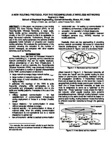
Fig. 1. (a) Transmission pattern of an omnidirectional antenna. (b) Transmission pattern of a directional antenna.

except that one. The paper also describes two schemes that use directional DATA/ACK and omnidirectional CTS, with sending the RTS signal omni-directionally or directionally. The relative performance of the two schemes is topology dependent. In [32], each node is assumed to have a switchedbeam antenna using a beamforming matrix. In [11], Fahmy et al present a scheme using omnidirectional RTS/CTS with steered beam antennas. In [6] and [35], a Directional Network Allocation Vector (DNAV) was used, which augments the NAV with a direction field. If a node receives an RTS or CTS from a certain direction, then it defers transmissions only in that direction. In [1] and [22], the angles are determined using signal strength information along with position information. The other category of MAC protocols for multihop wireless networks using directional antennas are TDMA-based schemes. In this approach, time is divided into frames which are in turn divided into slots that can be used for data transmissions. Slot scheduling is done in order to satisfy constraints to prevent exposed and hidden terminal problems among 1hop and 2-hop neighbors. The derivation of an optimal schedule is NP-complete [9][10][29]. A heuristic approach named UxDMA is presented in [25]. The framework specifies time, frequency, or code division in a multiple access channel assignment. However, the need for the collection of the complete network topology and for distributing the schedule reduces the scalability of this approach. In [8], Dyberg et al. analyze the performance of multihop wireless networks using TDMA MAC with beam steering and adaptive beamforming antennas. The authors use a centralized approach which is ill-suited for this type of network. A distributed protocol is presented in [2], which uses the 2-hop neighborhood to derive slot allocation schedules. The protocol presented in this paper is for the directional TDMA environment. It is different from the above protocols in that it is both on-demand, based on the dynamic source routing (DSR) protocol strategy, and distributed. Each node only needs to keep track of the slot allocation status of its 1-hop and 2-hop neighbors, as opposed to having information about the entire topology and slot allocation states of all of the nodes in the network. These characteristics enhance the efficiency and scalability of the proposed protocol. In addition, some researchers presented protocols for directional antennas in multihop wireless networks residing at the network layer. In [5], Choudhury and Vaidya present the DDSR (Directional Dynamic Source Routing) protocol. DDSR operates on top of the DiMAC (Directional Medium

Access Control) protocol which is an extension of 802.11 for directional antennas. The authors use the single switched directional antenna model. It has two modes of operation: omni-directional (referred to also as simply omni in this paper) and directional. In omni mode, after a signal is detected, the antenna determines the beam on which the received signal power is maximum. The rest of the dialog is carried out using this beam. In directional mode, a node can select only one of its beams and beamform with a specified directional gain. Considerable sweeping delays are incurred by the protocol due to sequential transmission of the same packet over different beams to cover 360◦ . The authors evaluate the impact of directional antennas in multihop wireless networks, and identify challenges which emerge due to the use of this technology. Their work suggests that directional antennas have decreased impact in dense or linear networks. Significant performance gains are realized in sparse and random topologies. In [30], Saha and Johnson present routing improvement techniques for multihop wireless networks using directional antennas. In their paper, directional antennas are used to bridge network partitions by transmitting selected packets over longer distances. In addition, the authors use the directional antennas to repair route breaks due to node movement, and reduce delivery latency by avoiding dropped packets and additional routing overhead. Their protocol is DSR-based. In [12], Jasani and Yen propose an improvement of DSR using directional antennas. The protocol focuses on preventive route maintenance by extending the life of a link using directional antennas. Preventive warnings are transmitted to the previous node in the path to create a directional antenna pattern. This is done when the received packet power goes below a certain minimal threshold. The authors name the process of switching from omni-directional transmission to directional transmission orientation handoff. Performance improvements are realized at the network layer by using the proposed scheme. The protocol in this paper is also DSR-based, but differs from the above protocols in the fact that it is designed for use in the TDMA environment, and for the MBAA directional antenna model. Bao et al [2] propose a Receiver-Oriented Multiple Access (ROMA) protocol, for networks using MBAA-antennas in a TDMA environment. ROMA uses the Neighbor-aware Contention Resolution algorithm (NCR) in [3]. Transmission and reception are done using directional antennas. In ROMA, nodes contend for shared resources (transmission slots in this case) and contention resolutions are based on the context number (slot number in this case) and node identifier. Nodes with the highest priorities among their contenders are elected to access the resource, or transmission slot, without conflict. The neighbor protocol in ROMA is used for topology maintenance which includes 2-hop topology information for each node and detection of neighbors. This is accomplished by employing short signals that use the omnidirectional mode of the antenna. ROMA is a distributed algorithm that allows the nodes to calculate their channel access schedules based on their 2-hop topology information. ROMA evenly splits nodes in the network into transmitters and receivers which are paired together to establish communication.

3

In [14], Jawhar and Wu present a race-free routing protocol for QoS support in TDMA-based multihop wireless networks. The protocol allows a source node to find and reserve a QoS path with a certain required bandwidth (which is translated into number of data slots) to a desired destination node. In this paper, the protocol is extended to allow the path reservation scheme to work in TDMA-based multihop wireless networks, where the nodes are equipped with directional MBAA-antennas. The remainder of the paper is organized as follows. Section 2 provides a discussion of related work to the protocol presented in this paper. Section 3 presents the assumptions and definitions used in the protocol. Section 4 presents the protocol along with the data structures, algorithms, and some detailed examples. Section 5 presents simulation results that demonstrate the efficiency of the protocol. The conclusions and future research directions are featured in Section 6.

(b)

(a)

Fig. 2. Transmission pattern of an MBAA antenna system with k=4 beams. Each of the k beams can be oriented in a different desired direction. The figure shows: (a) Beams in transmission mode. (b) Beams in reception mode.

a b

II. D IRECTIONAL A NTENNA S YSTEM A SSUMPTIONS AND D EFINITIONS In this paper, it is assumed that each node in the network is equipped with an MBAA-antenna system. Each antenna is capable of transmitting or receiving using any one of k beams which can be directed towards the node with which communication is desired [2][33][34]. In order for node x to transmit to a node y, node x directs one of its k antennas to transmit in the direction of node y, and node y in turn directs one of its k antennas to receive from the direction of node x. Radio signals transmitted by omnidirectional antennas propagate equally in all directions. On the other hand, directional antennas install multiple antenna elements so that individual omnidirectional RF radiations from these antenna elements interfere with each other in a constructive or destructive manner. This causes the signal strength to increase in one or multiple directions. The increase of the signal strength in a desired direction and the lack of it in other directions is modeled as a lobe. The angle of the directions, relative to the center of the antenna pattern, where the radiated power drops to one-half the maximum value of the lobe is defined as the antenna beamwidth, denoted by β [2]. With the advancement of silicon and DSP technologies, DSP modules in directional antenna systems can form several antenna patterns in different desired directions (for transmission or reception) simultaneously. Figure 1(a) shows the transmission patterns of an omnidirectional antenna. Figure 1(b) shows the transmission pattern of a directional antenna. In the multihop wireless network environment considered in this paper, each node is equipped with an MBAA antenna that is capable of receiving and transmitting one or more packets simultaneously by pointing the antenna beams toward the nodes with which it is communicating, while annulling all other undesired directions. The antenna system can either transmit or receive data at any given time, but cannot do both simultaneously. It is also assumed that the an MBAA antenna is capable of broadcast that covers a transmission range that is similar to that of the directional mode by adjusting the beam width

c

f d

g e

Fig. 3. antennas.

An example showing nodes communicating using directional

or by using the omnidirectional mode of the antenna at a lower frequency band. This broadcast capability can be used for control information communication as well as neighbordirection findings. Preston [24] presented operation modes for the directional antennas for finding the coarse as well as the precise angular location of a single and multiple sources. The angular position of a radiating source can be determined within one or two hundred microseconds depending on the signal processing speed. In this paper, it is assumed that an MBAA antenna system is capable of detecting the precise angular position of a single source for locating and tracking neighbor nodes. Figure 2 shows a node equipped with an MBAA antenna array with k=4 beams. Each of the k beams is able to be oriented in a different desired direction. Figure 2(a) shows the antenna array in the transmission mode, and Figure 2(b) shows the antenna array in the reception mode. The protocol presented in this paper uses the neighbor protocol proposed in [2] to acquire and maintain the two-hop neighbor information needed by the scheduling mechanism. Exchanging neighborhood information is not done using the directional antenna scheduling mechanism because the latter assumes a priori knowledge of the neighborhood. Therefore, neighborhood information is transmitted over a common channel on a best effort basis using the omnidirectional mode of the antenna system. This neighbor protocol uses a separate time section for exchanging its information. The collected control information is used by the nodes to later propagate route reservation control messages during the route discovery process. More details about the neighbor protocol can be found in [2].

4 16 15

1

14

2

d 13

b

e

c

y z

x

3

Fig. 5.

Illustration of allocation rule 2.

4

12

x z

y

5

11

6

10 9

7

Fig. 6.

Illustration of allocation rule 3.

8

Fig. 4. The horizon as seen by a node. The figure includes 16 segments and 16 angular groups.

Two nodes, x and y, are considered 1-hop neighbors if they are within each other’s directional range. In order for a node x to successfully transmit data to one of its 1-hop neighbor nodes, y, x must orient one of its transmitting beams in the direction of y, and y must orient one of its reception beams in the direction of x. Figure 3 shows a group of nodes communicating using MBAA directional antennas. In the figure, node d is transmitting to both b and e simultaneously using two different directional antenna beams. Also, node b is receiving from a and d simultaneously. Node g is transmitting to f . Note that even though node g’s transmission to f covers e, e does not have one of its receiving beams oriented towards g, and subsequently will not receive the data being transmitted to f . Each node x maintains information about the angular location (direction) of each of its 1-hop and 2-hop neighbors [2]. For simplicity, the nodes are assumed to be placed on a flat plane. As illustrated in Figure 4, the horizon of each node is divided into 360◦ /(β/2) = 720◦ /β segments, and every two continuous segments define one group. A segment corresponds to the minimum angular separation of two neighbors in order to receive two separate antenna beams without interference. Therefore, 720◦ /β groups exist. Each 1-hop neighbor y of x belongs to two groups that overlap at y. Ayx denotes the set of angular groups to which belongs the 1-hop neighbor y of x. Two nodes y and z are considered in the same angular direction with respect to a third node x if and only if Ayx ∩ Azx 6= φ. As an example, consider the nodes in Figure 4, where the horizon with respect to a node a is shown. According to the definition stated earlier, the set of angular groups for links (a,b), (a,c), (a,d) and (a,e) are Aba = {13, 14}, Aca = {14, 15}, Ada = {15, 16}, Aea = {1, 2}. Therefore, nodes b and c are considered in the same angular direction with respect to node a because Aba ∩ Aca = {14} 6= φ. Similarly, nodes c and d are considered in the same angular direction. However, nodes b and d, for example, are not in the same angular direction, since Aba ∩ Ada = φ. III. O UR P ROTOCOL The networking environment that is assumed in this paper is TDMA. In this environment, a single channel is used to

communicate between nodes. The TDMA frame is composed of a control phase and a data phase [4][18]. Each node in the network has a designated control time slot, which it uses to transmit its control information. However, the different nodes in the network must compete for the use of the data time slots in the data phase of the frame. Liao and Tseng [17] show the challenge of transmitting and receiving in a TDMA single channel omnidirectional antenna environment, which is non-trivial. In this section, the slot allocation rules for the TDMA directional antenna environment are presented. The hidden and exposed terminal problems make each node’s allocation of slots dependent on its 1-hop and 2-hop neighbor’s current use of that slot. This will be explained in a detailed example later in this paper. The model used in this protocol is similar to that used in [14] and [17], but includes modifications to support directional antenna systems. Each node keeps track of the slot status information of its 1-hop and 2-hop neighbors. This is necessary in order to allocate slots in a way that does not violate the slot allocation conditions imposed by the nature of the wireless medium and to take the hidden and exposed terminal problems into consideration. Below are the slot allocation conditions. A. Slot allocation conditions for directional antennas A time slot t is considered free to be allocated to send data from a node x to a node y if the following conditions are true: 1) Slot t is not scheduled to receive in node x or scheduled to send in node y, by any of the antennas of either node (i.e. antennas of x must not be scheduled to receive and antennas of y must not be scheduled to transmit, in slot t). 2) Slot t is not scheduled for receiving in any node z, that is a 1-hop neighbor of x, from node x where y and z are not in the same angular direction with respect to x (i.e. Ayx ∩ Azx 6= φ). 3) Slot t is not scheduled for receiving in node y from any node z, that is a 1-hop neighbor of x, where x and z

Fig. 7.

x

y

z

w

Illustration of allocation rule 4.

5

are in the same angular direction with respect to y (i.e. Axy ∩ Azy 6= φ). 4) Slot t is not scheduled for communication (receiving or transmitting) between two nodes z and w, that are 1-hop neighbors of x, where w and y are in the same angular y direction with respect to z (i.e. Aw z ∩ Az 6= φ), and x and z are in the same angular direction with respect to w (i.e. Axw ∩ Azw 6= φ). In Figure 5, which illustrates allocation rule 2, node x cannot transmit to node y using slot t because it is already using slot t to transmit to node z which is in the same angular direction as node y. In Figure 6, which illustrates allocation rule 3, node x cannot allocate slot t for sending to node y because slot t is already scheduled for sending from node z. Node z is a 1-hop neighbor of x, and Axy ∩ Azy 6= φ. In Figure 7, which illustrates allocation rule 4, slot t cannot be allocated to send from x to y because it is already scheduled for communication between two nodes z and w, that are 1-hop y z neighbors of x, where Axz ∩ Aw z 6= φ and Ax ∩ Ax 6= φ. B. The data structures The proposed protocol is on-demand, source based and similar to DSR [23]. Its on-demand nature increases its efficiency, since traffic overhead control is only needed when data communication between nodes is desired. Each node maintains and updates three tables; ST , RT and H. Considering a network with n nodes, and s data slots in the TDMA frame, in a node x, the tables are denoted by STx , RTx and Hx . The tables contain the following information: • STx [1..n, 1..s]: This is the send table which contains slot status information for the 1-hop and 2-hop neighbors. For a neighbor i and slot j, STx [i, j], is a structure which has two fields: (1) The state field: It can have one of the following values representing three different states: 0 free, 1 - allocated to send, 2 - reserved to send. (2) The angular groups field: It contains k sets of angular groups (one for each antenna). The entry A[a]ji denotes the set of angular groups to which the ath sending antenna is pointed. A[a]ji = φ is used to indicate that the ath antenna for neighbor i is not used during slot j. • RTx [1..n, 1..s]: This is the receive table which contains slot status information for the 1-hop and 2-hop neighbors. For a neighbor i and slot j, RTx [i, j], is a structure which has two fields: (1) The state field: It can have one of the following values representing three different states: 0 free, 1 - allocated to receive, 2 - reserved to receive. (2) The angular groups field: It contains k sets of angular groups. The entry A[a]ji denotes the set of angular groups to which the ath receiving antenna is pointed. Also here, A[a]ji = φ is used to indicate that the ath antenna for neighbor i is not used during slot j. • Hx [1..n, 1..n]: This table contains information about node x’s 1-hop and 2-hop neighborhood. Each entry Hx[i, j] is a structure, which has two fields: (1) The neighbor field: It contains a 1 if node i, which is a 1hop neighbor of node x, has node j as a neighbor, and contains a 0 otherwise. (2)The angular group field: Aji ,

p

l c a

j o n

k

e

q

f s

b m

g

i

d h r

Fig. 8. A detailed example showing the allocation of slots 1 and 2 at node b. Bold cones show transmissions/receptions in slot 1 and plain cones show transmissions/receptions in slot 2. The circle indicates the directional range of node b. a

Node Slot

c

b

S1 S2

d

e

g

f

S1 S2 S1 S2 S1 S2 S1 S2

S1 S2 S1 S2

i

h

S1 S2 S2 S2

S/R

S

R

S

S

S

S

R

R

A1

{4,5}

{12,13}

{5,6}

{1,2}

{1,16}

{1,16}

{13,14}

{8,9}

A2

{1,16}

{8,9}

{12,13}

{4,5}

Node Slot

k S1

m

l

n

S2 S1 S2 S1 S2 S1 S2

o

{8,9}

p

q

S1 S2 S1 S2

S1 S2

r

s

S1 S2 S1 S2

S/R

S

R

S

R

R

S

R

A1

{1,2}

{9,10}

{5,6}

{8,9}

{4,5}

{1,2}

{12,13}

A2

Fig. 9. The allocation table, which corresponds to the detailed example showing the allocation of slots 1 and 2 at node b.

which contains the set of angular groups to which node j belongs. It is important to note at this point that in the following definitions and algorithms, the word “slot” implies a “slot in a particular direction using the associated antenna”. For example, each of the slot timers defined later in this paper is associated with a particular slot/antenna pair. C. The QoS path reservation algorithm When a node S wants to send data to a node D, with a bandwidth requirement of b slots, it initiates the QoS path discovery process. Node S determines if enough slots are available to send from itself to at least one of its 1-hop neighbors. If so, it broadcasts a QREQ(S, D, id, b, x, P AT H, N H) to all of its neighbors. The message contains the following fields: 1) S: ID of the source node. 2) D: ID of the destination node.

6

3) id: Message ID. The (S, D, id) triple is therefore unique for every QREQ message and is used to prevent looping. 4) b: Number of slots required in the QoS path from S to D. 5) x: The node ID of the host that is forwarding this QREQ message. 6) P AT H: A list of the form ((h1 , l1 ), (h2 , l2 ), ..., (hk , lk )). It contains the accumulated list of hosts and time slots, which have been allocated by this QREQ message so far. hi is the ith host in the path, and li is the list of slots used by hi to send to hi+1 . Each of the elements of li contains the slot number that would be used, along with the corresponding the set of angular groups, Ai+1 , which i represents the direction in which the sending antenna of host i must be pointed, during that slot, to send data to host i + 1. 0 0 0 0 0 7) N H: A list of the form ((h1 , l1 ), (h2 , l2 ), ..., (hk , 0 lk )). It contains the next hop information. If node x is forwarding this QREQ message, then NH contains a list 0 0 of the next hop host candidates. The couple (hi , li ) is the ID of the host, which can be a next hop in the path, along with a list of the slots, which can be used to send 0 0 data from x to hi . li is a list of the slots to be used to send from host i to host i + 1 along with the angular 0 group for each slot. li has the same format as li in PATH. 8) M ax QREQ node wait time, M ax QREQ tot wait time, and M ax QREQ QREP tot wait time: QREQ message wait timing constraints, which are specified by the application. Each timer will be discussed in more detail in a later section. When an intermediate node receives the QREQ message, it composes the NH list which includes the neighbors with which it has a link that contains at least b free slots in the corresponding direction. The message is then forwarded to these neighbors. If the QREQ message reaches the destination node D, it means that a QoS path from S to D was discovered and that there were at least b free slots available to send data from each node to each subsequent node along this path. These slots are now marked as allocated in the ST and RT tables of the corresponding nodes. Subsequently, node D unicasts a reply message, QREP (S, D, id, b, P AT H, N H), to node S. This message is propagated along the nodes indicated in P AT H. As the QREP message travels back to the source node, all of the intermediate nodes along the allocated path must confirm the reservation of the corresponding allocated slots (i.e. change their status from allocated to reserved). The timing and propagation of the QREQ and QREP messages are controlled by timers, a queueing process, and synchronous and asynchronous slot status broadcasts, which are discussed in detail later in this paper. D. A detailed example of slot allocation at an intermediate node Figure 8 and the corresponding table in Figure 9 provide an example of the slot allocation considerations at an intermediate node b. In the example, node b receives a QREQ message from node a and is determining to which of its 1-hop neighbors it

can extend the QREQ message. The example illustrates the considerations for slots 1 and 2 of the TDMA frame. The portion of the allocation table for slots 1 and 2 at node b is shown in Figure 9. In this example, slot 1 is reserved to send from node a to node b and node p. Slot 1 is also reserved to send from node d to node q, and from node d to node b, simultaneously, for different QoS paths. These reservations of the same slot to send from the same node to multiple nodes, for different QoS paths, is not possible in an omnidirectional antenna system. This demonstrates the significant spatial reuse that can be achieved in the directional antenna environment. According to rule 1 of the slot allocation conditions, slot 1 cannot be allocated by node b to send to any of its neighbors on any of its antennas because this slot is already scheduled to receive by node b (from nodes a and d). Let’s consider the possibility of allocating slot 2 to send from node b to each of its neighbors. According to rule 1, slot 2 cannot be allocated to send from b to i because it is already scheduled to send for another QoS path. Also, according to the same rule, slot 2 cannot be scheduled to send from node b to e because slot 2 is already scheduled to send by node e. Namely, it is scheduled to send from node e to nodes j and s for different QoS paths which is another illustration of the spatial reuse that is afforded to directional antenna systems. According to rule 2 of the slot allocation conditions, node b cannot allocate slot 2 to send to node g because slot 2 is already scheduled to send from node b to node i, where Aib ∩ Agb 6= φ (i.e. node i is in the same angular direction as node g with respect to node b). Also, according to rule 3, slot 2 cannot be allocated by node b to send to node h. This is because this slot is already scheduled to receive in node h from node m, b where Am h ∩Ah 6= φ. Note that slot 2 is also scheduled by node h to receive from r on a different antenna without preventing the use of the same slot to send from node m to node h. According to rule 4, slot 2 cannot be scheduled to send from node b to c because it is already scheduled to send from l to k, where (Alk ∩ Ack 6= φ) and (Abl ∩ Akl 6= φ). According to the same rule, and because of the same reason, slot 2 cannot be scheduled to send from b to k or from b to l. As a result, node b is able to allocate slot 2 to send to nodes f , n, and o. E. An example of multiple QoS paths passing through common nodes Figure 10 shows an example with three different reserved QoS paths: abcdef g (path 1), hicjek (path 2), and njml (path 3). The three paths share several common nodes. Namely, nodes c and e are common between paths 1 and 2, and node j is common between paths 2 and 3. Due to the use of directional antenna systems, these common nodes are able to receive different data belonging to different paths from multiple directions in the same data slot without interference. Similarly they can transmit to different nodes belonging to different paths in different directions in the same data slot as well. This scenario is not possible in the omnidirectional antenna environment, and illustrates the potential increase of network throughput in multihop wireless networks using directional antennas.

7

b

g d

a

c e i

h

f

j m k

l

n

Fig. 10. An example showing three QoS paths: abcdef g, hicjek, and njml.

F. Wait timers We define the following timers, which control the allowable delay of the propagation of the QREQ and QREP messages through the system. These timers can be initialized to a tunable value which can vary according to the requirements of the application being used. It is also possible to disable some of these timers, which are specified below, if the application does not have such delay requirements. TTL allocated slot time. Each slot t in ST and RT tables has a T T Lt (Time to Live) count down timer associated with it. This T T Lt timer is only needed when the slot is set from free to allocated. As soon as a slot is converted from free to allocated, its TTL timer is set to a certain “time to live” parameter. This is a tunable parameter, which can be determined according to the application needs. The T T Lt timer is set to 0 upon initialization and when the slot becomes free. When the status of a slot t is changed from free to allocated due to a QREQ, which is processed by the node, the T T Lt timer is initialized to a predetermined T T L allocated slot time. This time should be at least equal to the RTT (Round Trip Time) for a QREQ to come back as a QREP. This time is a tunable parameter which can be fixed according to the application requirements and/or the network size and/or density. It can be increased with a larger number of nodes in the network. A reasonable value could be 2∗RT T , but it could be set to a smaller or larger value depending on the size and propagation delay characteristics of the network involved. A large value for this T T Lt timer corresponds to a conservative strategy. If it is too large, a slot would have to wait too long to automatically convert back to free. That lengthens the path acquisition time for a QREQ, which might not be desirable in certain applications. On the other hand, if the TTL time is too small, then a node will be too anxious to return allocated slots to the “free” status before the reservation is confirmed with a QREP message. This creates a risk of converting a slot back to free status too soon. After a short amount of time, the corresponding QREP message of the QREQ message that initially allocated this slot comes back. However, the slot which was changed to free can now be allocated for another path. This way, double allocation of the same slot exists for two different paths, and this leads to a racing condition, the very condition the protocol strives to avoid.

Explicit de-allocation message from the destination. In addition to the above soft allocation timer strategy, further performance improvements can be achieved by having an explicit deallocation message issued as a flood from the destination to the source. This message is initiated by the destination when it receives as soon as a QoS path is discovered. The reception of the de-allocation message by the nodes in the network will cause the immediate de-allocation of the slots which were not used in the final path(s). This increases the utilization and efficiency of the network. We incorporated both the soft deallocation timer as well as the explicit de-allocation message in the protocol. TTL reserved slot time. When a slot is reserved (i.e. its allocation is confirmed and it is in reserved status) for a particular QoS path, it must be used for actual data transmission within a certain time-out period which we define as the T T L reserved slot time. This time is a parameter which can be set according to the application and network environment involved. If at any time a slot is not used for data transmission for more than this time, it must be returned to free status. This is done in the following manner. The associated timer is refreshed each time the slot is used for data transmission. The timer is constantly counted down. If this timer reaches zero at any time then the slot is returned back to f ree status. This timing is also useful for a situation where the QREP message used to confirm a slot reservation is successful in propagating from the destination through some nodes, but is not then forwarded to the source. In this case, the nodes which already confirmed the reservation of their slots will still be able to return these slots back to the “free” status after this time-out period. Max QREQ node wait time. The QREQ can wait at an intermediate node for a maximum amount of time M ax QREQ node wait time. This is a parameter that is set to a tunable value according to the application and network requirements and characteristics. A reasonable value can be equal to 2 ∗ RT T . Its effect is similar to what was described earlier in the T T L allocated slot time section. Namely, it can vary according to a conservative or aggressive strategy. Also it depends on the size and propagation delay characteristics of the network. Furthermore, this time affects the QoS path acquisition latency which might be limited depending on the application involved. Max QREQ tot wait time. Another related delay type is the QREQ total wait time. This is the maximum allowable cumulative wait delay for the QREQ as it propagates through the network. This delay is controlled by the timer max QREQ tot wait time. This timer is decremented at each node according to the time the QREQ had to wait at that node, and it is forwarded along with the QREQ to the next node. Max QREQ QREP tot wait time. A third timer can be defined as M ax QREQ QREP tot wait time. This is the total time for path acquisition (QREQ propagation + QREP propagation); this time is also decremented by each node accordingly and forwarded along with the corresponding QREQ and QREP as they propagate through the system. Whenever a

8

node is forwarding a QREQ or a QREP message, it checks this time. If it is zero, then this means the QoS path reservation process has taken longer than the maximum allowable time and the corresponding QREQ or QREP message should now be dropped. Furthermore, the protocol can also take one of the following actions: (1) Send a notification message to all of the nodes along the reserved path (the nodes which forwarded the QREP message from the destination to this node) to return the corresponding slots which have been allocated and/or reserved by this path to free status. Or (2) Let those alreadyreserved-slots time out to free status as described by the T T L reserved slot time defined earlier. The M ax QREQ node wait time, M ax QREQ tot wait time, and M AX QREQ QREP tot wait time timers are optional and can be set to different values, according to their importance and/or criticality in the application that is being used. Similar timing techniques can be employed for the transmission of data packets as well. Timing might be even more significant as a requirement and in its effect over the performance of different applications, such as multimedia, voice, and video. Such applications are known to have strict requirements on the total delay permitted for a data packet. This is due to the fact that the packet can hold voice or video frames that must be delivered within a certain amount of time beyond which they become useless and must simply be discarded. G. Status broadcasting and updating There are two types of node status broadcasts: synchronous (periodic) and asynchronous. Synchronous periodic status updates. Each node broadcasts its slot allocation status (the ST and RT table information updates) to its 1-hop and 2-hop neighbors (i.e. with a 2-hop TTL). This broadcast is done periodically (synchronously) according to a predetermined periodic slot status update frequency. We define this as periodic status update time. These periodic updates enable the nodes to maintain updated neighborhood information as nodes come within or go out of their range. Furthermore, these updates inform the node of its neighbor’s slot status information on a periodic basis. When a node does not receive any synchronous (periodic) or asynchronous (due to changes in slot status) updates from a neighbor after a time-out period, which we call Status update tot, it will assume that this node is no longer one of its 1-hop or 2-hop neighbors, and will delete that neighbor from its ST and RT tables. Asynchronous status updates. The status update is done asynchronously as the status of slots is changed from free to allocated, or from allocated to reserved. There is no need to inform the neighbors of the change from allocated to free which results from TTL timer expiration. The neighbors will count down the time of the allocated slots as well and will change them to free status (i.e. will assume that the corresponding neighbor node will have done that) if no reservation change is indicated from the corresponding neighbor node. Note that the status updates are done with a 2-hop TTL flood to the 1-hop and 2-hop neighbors.

The asynchronous updates of receive and send slot status with the three state information, which includes the allocated status, solves the parallel reservation problem stated earlier in the paper, and eliminates the associated race condition which is caused by it; this was not done in previous research. When the 1-hop neighbor receives a separate and different QREQ, it will now be aware of the f ree/allocated/reserved status of its neighbors’ slots, rather than just their f ree/reserved status. This way, it will consider only slots which are totally free according to slot selection and will prevent the related race condition from occurring. This consideration is addressed in the select slot() function which is described later in this paper. H. The main algorithm at an intermediate node The protocol uses three states per slot to avoid any race conditions when multiple routes that pass through common nodes are being reserved at the same time. The possible race conditions and their remedies, which are similar for omnidirectional and directional antenna environments, are described in detail in [14]. When a node y receives a broadcasting message QREQ(S, D, id, b, x, P AT H, N H) initiated by a neighboring host x, it checks to determine whether it has received this same source routed request (uniquely identified by (S, D, id)) previously. If not, y performs the following steps. If y is not a host listed in NH then it exits this procedure. Otherwise, it calculates the values of the variables N U yz, AN U yz, and F yz, which are defined in the following manner: • N U yz: The number of slots that are not-usable for sending from y to z. This means that at least one confirmed reservation exists at y or one of its neighbors, which does not allow slot t to be used from y to send to z. This is due to any violation of any of the three slot allocation conditions. • AN U yz: The number of slots that are allocated-notusable for sending data from y to z. A slot is called AN U (allocated-not-usable) if there exist totally allocated reservations at y or its neighbors, which do not allow slot t to be used from y to send to z. This could be due to any violation of any of the three slot allocation conditions. However, violations of any of the lemma conditions are only (and totally) due to pure allocations (not confirmed reservations) at y and/or its neighbors. • F yz: The number of slots that are free at a node y to send to a node z respectively. This means that this slot is currently completely available to be used for sending from node y to node z and therefore satisfies all three of the slot selection conditions. Therefore, at node y, it is necessary to determine a separate set of N U yz, AN U yz, and F yz for each neighbor z of y. When a node y receives a QREQ message from a node x, it uses algorithm 1 which is shown below to forward the message, or to insert it in the QREQ pending queue, or to drop it. Algorithm 1 works in the following manner. When a QREQ message arrives at a node y from a node x, it does the

9

following. The algorithm first updates the ST and RT tables with the information in PATH. Then, it uses three routines to calculate N U yz, AN U yz, and F yz from ST and RT tables. Note that calculating these values would have taken into account all of the slot allocation rules described earlier. Afterwards, the algorithm initializes the next hop list N H temp to empty, and then attempts to build it by adding to this list each 1-hop neighbor z of y which has b slots free to send from y to z. The algorithm uses the select slot function which allocates slots using the slot allocation rules and the information in the updated ST and RT tables. There are three possible conditions that can take place. If at least one neighbor z of y has b slots free to send from y to z, this is called condition1, then the N H temp list will not remain empty and the node y will broadcast (i.e. forward) the QREQ message after incorporating the node x and the list li0 (i.e. the list of slots used to send from x to y) PATH (using P AT H temp = P AT H | (x, li0 ) ). Here, | means concatenation. Otherwise, if the N H temp list is empty after checking all of the neighbors, then that means that there are no neighbors z of y which have b slots free to send from y to z according to the slot selection conditions. At this point, the algorithm tries to determine if there is any “hope”, i.e., if there is at least one 1-hop neighbor z of y which has the condition (F yz +AN U yz) ≥ b. This would be condition2. In this case, the algorithm checks if the maximum time left for the required allocated slots to become free (or reserved) does not exceed the maximum total wait time left for this QREQ message (M ax QREQ tot wait time), then this QREQ message is placed in the QREQ pending queue. This queue will be scanned each time a slot becomes free to see if at that point, the QREQ message can be forwarded. This queue will be discussed in more detail later in this paper. If on the other hand, no 1-hop neighbor z of y has a condition of (F yz + AN U yz) ≥ b then there is “no hope” at the current time. Therefore, the QREQ message is dropped. I. The select slot function The select slot(y, z, b, ST, RT ) function will return a list of slots that are available to send from node y to z. As described earlier, it will do so according to the slot allocation rules, and the slot status information which is in the updated ST and RT tables. select slot() will return an empty list if b slots are not available to send from node y to z. J. The QREQ pending queue The QREQ’s that are waiting for slots to become free are placed in a QREQ pending queue. While waiting for the status of the different slots in the table to change, some slots will be freed and others will be confirmed. Every time a change in slot status is done (due to timer expiration, or confirming a reservation), the queue is scanned. Scanning the QREQ pending queue. Every time the queue is scanned, all QREQ messages, which have any of their corresponding wait timers expired, are deleted from the queue. These timers are: M ax QREQ node

Algorithm 1 The main algorithm at an intermediate node When a node y receives a QREQ message Update the ST and RT tables with the information in PATH N H temp = φ for each 1-hop neighbor node z of y do N U yz = calcR(z, ST, RT ) AN U yz = calcA(z, ST, RT ) F yz = calcF (z, ST, RT ) if F yz ≥ b then L = select slot(y, z, b, ST, RT ) if L 6= empty then N H temp = N H temp(z, L) | (z, L) else Error: cannot have F yz ≥ b and L = empty end if end if end for if N H temp 6= φ then 0 0 0 Let (hi , li ) be the entry in NH such that hi =y 0 let P AT H temp = P AT H | (x, li ) broadcast QREQ(S, D, id, b, x, P AT H temp, N H temp) message else for each 1-hop neighbor node z of y do if (F yz + AN U yz) ≥ b then let tmas = maximum time lef t f or required allocated slots to become f ree (or reserved) if max QREQ tot wait time ≥ tmas then insert QREQ message in QREQ pending queue exit this procedure end if end if end for end if

wait time, M ax QREQ QREP tot wait time, and M ax QREQ tot wait time. Also, for each QREQ in the queue, the new values for F yz, AN U yz, and N U yz are calculated, and it is determined under which conditions the new QREQ status falls. There are three possibilities: • Changed to condition 1 (i.e. now F yz ≥ b): In this case, forward the pending QREQ and delete the QREQ from the QREQ pending queue. • Changed to condition 2 (i.e. now (F yz + AN U yz) ≥ b): In this case, leave the corresponding QREQ in the QREQ pending queue. • Changed to condition 3 (i.e. (F yz + AN U yz) < b): In this case, delete the corresponding QREQ from the QREQ pending queue (i.e. drop this QREQ message). Here another policy can be adopted which would be to send a reject message back to the source of the QREQ to inform it of the rejection if the protocol requires informing the source nodes of the failing QREQ. If the TTL for an allocated slot expires, this means that the slot has been allocated for too long and not confirmed (i.e. reserved) by a QREP message. In this case, the corresponding slot status in ST and and RT tables is set to f ree. If the status of a QREQ message in the queue changes into condition 1, then the algorithm calls the select slot() function for all nodes that are 1-hop neighbors of y. It then builds the next hop list accordingly, which will include every neighbor

10

node z, for which there are b slots available to send from y to z, and the list of these slots. This is done using Algorithm 2. Algorithm 2 Forwarding the QREQ message from the QREQ pending queue N H temp = φ for every 1-hop neighbor z of y do L = select slot(y, z, b, ST, RT ) if L 6= φ then N H temp = N H temp | (z, L) end if end for if N H temp 6= φ then 0 0 0 let (hi , li ) be the entry in NH such that hi =y 0 let P AT H temp = P AT H | (x, li ) broadcast QREQ(S, D, id, b,y, P AT H temp, N H temp) delete QREQ message from the QREQ pending queue end if

The QREQ message is forwarded by the intermediate nodes that are able to allocate b slots to send data and can therefore be a part of the QoS path that is being discovered and reserved. As the QREQ message propagates from the source to the destination, the slot reservation information is not updated in the ST and RT tables. This unconfirmed reservation information is only maintained and updated in the QREQ message as it propagates through the nodes. The status of the corresponding slots in the ST and RT tables in the nodes continues to be f ree. This can lead to multiple reservations of the same slots by different QREQ messages due to a race condition, which is explained later in this paper. If and when the QREQ message arrives at the destination node D, then indeed, a QoS path to send data from S to D with b slots in each hop was discovered. In this case, the destination D replies by unicasting a QREP (S, D, id, b, P AT H, N H) back to the source, which confirms the path that was allocated by the corresponding QREQ message. The QREP message propagates from D to S through all of the intermediate nodes that are specified in PATH. PATH contains a list of the nodes along the discovered path along with the slots which were allocated for this path at each node. As the QREP message propagates through the intermediate nodes, each node updates its ST and RT tables with the slot reservation information in the QREP message and changes the status of the corresponding slots to reserved. This represents the confirmation of the reservation of the slots for the discovered path. IV. P ERFORMANCE A NALYSIS In order to verify and analyze the performance of the presented protocol, simulation experiments were conducted. A. Simulation Basically, the simulator starts by generating an area with certain dimensions, then randomly places a pre-determined number of nodes in the area. The nodes have a certain transmission range. From the placement of the nodes and their range a graph is generated. Then the simulator generates a number of data messages with a certain length for each

TABLE I PARAMETERS FOR THE DIRECTIONAL ANTENNA PROTOCOL SIMULATION Parameter Network Area Number of Nodes Transmission Range Bandwidth Data Packet Size Number of Data Slots Number of Sessions Average Message Length MAX SLOT RES TIME MAX SLOT ALLOC TIME MAX B

Value 300 × 300 m2 30 115 m 2 M b/s 512 bytes 30 20 100 M B 10980 ms 1350 ms 4 slots

message (different distributions can be used). Each message has a random source and destination pair. The arrival times of the messages is according to a Poisson process with a certain mean inter-arrival time. When the data message is processed by the source, it generates a QREQ message to discover a QoS path to the corresponding destination. The QREQ message is propagated through the nodes according to the proposed algorithm. Each node has a routing table as well as all of the tables needed for the algorithm (ST , RT , H, routing table, all of the required slot data structures, etc.). When the source receives the QREP message, it starts data transmission. The simulations are done for three different cases: (1) 1 antenna representing the omnidirectional antenna case (dir = 1, angle of coverage = 360◦ ), (2) 2 antennas (dir = 2, angle of coverage = 180◦ per antenna). (3) 4 directional antennas (dir = 4, angle of coverage = 90◦ per antenna). B. Simulation parameters A set of simulation experiments were performed. Table I shows a sample of the simulation parameters used in the experiments. The results for two sets of experiments are shown. Figures 11 and 12 contain the results for the first set of experiments, and figures 13 and 14 contain the results for the second set of experiments. The number of nodes (n) is 30 in an area of 300x300 m2 . The total number of data slots in the frame (dsn) is 30. The number of slots required for each session is a random number with a uniform distribution and a range from 1 to 4 slots (1 to max b). The range of each node is 115 m. The session (or data message) arrival is a Poisson process with a mean which was varied from 1 to 10 messages/sec. The message length is randomly selected according to a uniform distribution with a range from 0 to 10 Mbytes for the first set of experiments, and from 0 to 100 Mbytes for the second set of experiments. C. Simulation results and analysis Several performance measures were computed as the traffic rate (messages/second) is varied. The measured parameters are the overall percentage of packets received successfully, the average number of requests per successful acquisition of QoS path, the average number of requests per session, and the average QoS path acquisition time. In both sets of experiments, it can be observed that the average overall percentage of successfully received packets

11

Simulation Restults: n=30, message=10Mb, dsn=30, max_b=4, range=115m, area: 300x300m Varying data message rate in (mess./sec)

7.00 22.16 41.40 75.27

8.00 24.07 42.63 77.86

9.00 23.27 38.16 78.67

10.00 19.26 39.51 79.36

Avg. 27.70 44.53 81.80

Overall % of Successful Packets Data Rate 1.00 2.00 3.00 1 dir 42.56 39.36 29.20 2 dir 51.00 53.48 46.79 4 dir 86.31 85.05 78.75

7.00 25.60 43.70 81.85

8.00 21.69 35.92 78.78

9.00 18.70 34.09 80.61

10.00 22.10 41.67 74.63

Avg. 27.89 43.02 80.92

Average Number of Requests Per Successful Aquisition of QoS Path Data Rate 1.00 2.00 3.00 4.00 5.00 6.00 7.00 1 dir 1.51 1.65 1.73 1.73 1.69 1.65 1.58 2 dir 1.34 1.41 1.48 1.43 1.46 1.45 1.47 4 dir 1.28 1.33 1.39 1.41 1.35 1.39 1.37

8.00 1.71 1.42 1.46

9.00 1.64 1.49 1.34

10.00 1.65 1.45 1.39

Avg. 1.65 1.44 1.37

Average Number of Requests Per Successful Aquisition of QoS Path Data Rate 1.00 2.00 3.00 4.00 5.00 6.00 7.00 1 dir 1.61 1.69 1.64 1.71 1.78 1.65 1.64 2 dir 1.33 1.41 1.50 1.45 1.52 1.49 1.43 4 dir 1.29 1.38 1.48 1.41 1.42 1.36 1.40

8.00 1.60 1.43 1.41

9.00 1.64 1.40 1.36

10.00 1.64 1.38 1.40

Avg. 1.66 1.43 1.39

Average Number of Requests per Session Data Rate 1.00 2.00 3.00 4.00 1 dir 2.33 2.51 2.60 2.64 2 dir 2.11 2.20 2.32 2.32 4 dir 1.44 1.51 1.60 1.69

Fig. 11.

4.00 16.08 9.80 9.30

5.00 25.04 43.02 82.01

6.00 22.30 49.13 76.19

5.00 2.66 2.35 1.65

6.00 2.70 2.26 1.76

7.00 2.69 2.36 1.77

8.00 2.70 2.35 1.82

9.00 2.70 2.42 1.70

10.00 2.73 2.38 1.72

Avg. 2.62 2.31 1.67

Average Number of Requests per Session Data Rate 1.00 2.00 3.00 4.00 1 dir 2.40 2.48 2.60 2.65 2 dir 2.15 2.18 2.30 2.36 4 dir 1.53 1.62 1.79 1.68

5.00 15.30 10.42 8.10

6.00 14.34 10.31 8.94

7.00 13.01 10.58 8.55

8.00 15.80 9.63 10.50

9.00 14.28 11.03 7.83

10.00 14.34 10.12 8.94

Avg. 14.52 10.00 8.53

Avgerage QoS Path Acquisition Time Data Rate 1.00 2.00 3.00 1 dir 13.54 15.30 14.26 2 dir 7.71 9.45 11.24 4 dir 6.73 8.71 10.92

Simulation results table. Data message length: 10MB

Overall % of Successful Pakets

40

2.5 2 1.5 1

1 dir 2 dir 4 dir

0 1

2

1 dir 2 dir 4 dir

0.5 0 3 4 5 6 7 8 Data Message Rate (mess/sec)

9

10

1

2

(a) Average # of Requests per Session

Acq. time (sec)

2.5 2 1.5 1

0 1

2

9

9

10

Avg. 2.62 2.33 1.69

5.00 17.29 11.62 9.69

6.00 14.50 11.11 8.38

7.00 14.29 9.81 9.17

8.00 13.32 9.77 9.39

9.00 14.25 9.03 8.24

10.00 14.12 8.79 9.12

Avg. 14.67 9.88 8.97

Average # of Requests per Successful Path Acquisition 3

1 dir 2 dir 4 dir 1

10

2

20

3 4 5 6 7 8 Data Message Rate (mess/sec)

9

10

1

2

9

10

drops as the traffic rate is increased. Also, as expected by the theoretical analysis, this percentage is consistently the smallest in the omnidirectional case (dir = 1). For example, in the first set of experiments presented in the table in Figure 11, the overall percentage of successfully received packets ranges from 45.64 for a mean traffic rate of 1 messages/sec down to 27.70 for a mean traffic rate of 10 messages/sec. This percentage is higher with the two-antenna case and ranges from 53.69 down to 44.53. The highest percentage is obtained in the four-antenna case which ranges from 90.59 down to 81.80. Also, as expected by the theory, the simulation shows that the average number of requests per successful acquisition of a QoS path, the total number of requests per session (i.e. including sessions that were not able to acquire a path), and the average QoS path acquisition time are consistently higher for the omnidirectional case, followed by the two-antenna and the

9

10

9

10

Average QoS Path Acquisition Time 40

3.5

35

3

30

2.5 2 1.5

1 dir 2 dir 4 dir

25 20 15 10

1 dir 2 dir 4 dir 1

2

5 0 3 4 5 6 7 8 Data Message Rate (mess/sec)

(c)

(d)

Simulation results. Data message length: 10MB

3 4 5 6 7 8 Data Message Rate (mess/sec)

(b)

4

0 3 4 5 6 7 8 Data Message Rate (mess/sec)

1 dir 2 dir 4 dir

0

1

2

1 0.5

Average # of Requests per Session

30

1

2 1.5

(a)

0 3 4 5 6 7 8 Data Message Rate (mess/sec)

10.00 2.69 2.30 1.80

40

0.5

(c) Fig. 12.

3 4 5 6 7 8 Data Message Rate (mess/sec)

10

1 dir 2 dir 4 dir

0.5

9.00 2.72 2.43 1.66

60

0

# of Requests

40

3

8.00 2.69 2.45 1.73

2.5

20

1 dir 2 dir 4 dir

3.5

7.00 2.66 2.31 1.69

80

Average QoS Path Acquisition Time 50

6.00 2.66 2.41 1.69

Simulation results table. Data message length: 100MB

(b)

4

5.00 2.68 2.39 1.73

Overall % of Successful Pakets

% Succ. Packets

# of Requests

% Succ. Packets

60

6.00 25.72 39.05 79.50

100

3 80

4.00 15.81 10.28 9.41

5.00 25.96 41.79 81.15

120

3.5

100

# of Requests

Fig. 13.

Average # of Requests per Successful Path Acquisition 4

120

20

4.00 27.99 42.68 82.60

# of Requests

Avgerage QoS Path Acquisition Time Data Rate 1.00 2.00 3.00 1 dir 11.39 14.56 16.12 2 dir 7.91 9.28 10.90 4 dir 6.65 7.69 8.83

4.00 26.88 44.28 82.48

Acq. time (sec)

Overall % of Successful Pakets Data Rate 1.00 2.00 3.00 1 dir 45.64 36.96 31.42 2 dir 53.64 49.74 43.84 4 dir 90.59 88.98 86.64

Simulation Restults: n=30, message=100Mb, dsn=30, max_b=4, range=115m, area: 300x300m Varying data message rate in (mess./sec)

Fig. 14.

9

10

1

2

3 4 5 6 7 8 Data Message Rate (mess/sec)

(d)

Simulation results. Data message length: 100MB

four-antenna cases. This is due to the fact that it is increasingly easier for the network to acquire a QoS path as the number of antennas increases. The second set of experiments, which were done for a longer data message length of 100 Mbytes, shows a decrease in the overall percentage of successfully received packets due to the increase in total traffic. The overall percentage of successfully received packets, and path acquisition time measurements follow the same trends as the first set of experiments showing a considerable advantage with the increase in number of antennas. This confirms the same analysis and reached conclusions. These simulation results clearly demonstrate the increased efficiency and performance of the network as the number of directional antennas increases. As was indicated earlier, this increased performance is due to the considerable increase in spatial reuse and the ability for each node to simultaneously

12

send or receive data in different directions. This functionally increases the effective number of data slots by a multiple of the number of antennas (or directions) used. This effect significantly improves performance. As the data shows, the increase in performance, or speed-up factor, when the number of antenna is increased by a factor of 2 (i.e. doubled from 1 to 2, and then from 2 to 4) is significant (speed up factor > 1). As expected, however, it is still below the theoretical speed-up factor of 2. For the first set of experiments for example, the data shows that that ratio of the overall average percentage (average for all data traffic rates) of successful packets of the two-antenna case to the one-antenna case is 1.61, which is > 1 and < 2. The ratio of the four-antenna case to the twoantenna case is 1.84, which is also > 1 and < 2, and the ratio for the four-antenna case to the one-antenna case is 2.95 which is < 4. This is to be expected from the theory of parallel and distributed systems because the actual speed-up factor is always below the ratio of the number of parallel units, or antennas, in this case. D. Additional directional antenna tradeoffs and future research It is worthy of noting at this point, that in highly mobile MANETs (Mobile Ad Hoc Networks), more overhead would be needed to discover, exchange and maintain topology information between nodes. In the directional antenna environment, this overhead would be higher than that of the omnidirectional case. However, the gain realized due to the significant increase in spatial reuse, power savings, reduced path hop count, reduced end-to-end delay, and higher throughput offsets this increase. The effects of mobility on this protocol as well as optimization techniques employed to reduce this overhead is a rich area of future research in this field, and is currently being investigated. Additionally, this protocol is a heuristic approach to a directional antenna version of the scheduling problem in the TDMA environment, which has been proven to be NP-complete [10][13][19][21]. Theoretical bounds and comparison with optimal path assignment is another possible area of future research. V. C ONCLUSIONS In this paper, a protocol for TDMA-based bandwidth reservation for QoS routing in multihop wireless networks using directional antennas was presented. The protocol takes advantage of the significant increase in spatial reuse provided by the directional antenna environment, which drastically increases the efficiency of communication in this type of network. This is due to the reduction in signal interference and the amount of power necessary to establish and maintain communication sessions. The simulation results clearly show a significant gain in performance with an increase in the number of successfully received packets, as well as a decrease in the QoS path acquisition time. However, as expected, this gain in performance is still below the theoretical speed-up factor. In the future, we intend to improve this protocol through the employment of additional optimization techniques. In addition, we intend to preform more simulations in order to further

study, analyze and improve the performance of the protocol under different network environments and traffic conditions. R EFERENCES [1] S. Bandyopadhyay, K. Hasuike, S. Horisawa, and S. Taware. An adaptive MAC and directional routing protocol for ad hoc and wireless network using ESPAR antenna. Proceedings of ACM MOBIHOC, Long Beach, California, October 2001. [2] L. Bao and J. J. Garcia-Luna-Aceves. Transmission scheduling in ad hoc networks with directional antennas. Proc. of the 8th annual international conference on mobile computing and networking, pages 48–58, September 2002. [3] L. Bao and J.J. Garcia-Luna-Aceves. A new approach to channel access scheduling for ad hoc networks. In Proc. ACM Seventh Annual International Conference on Mobile Computing and Networking, Rome, Italy, July 2001. [4] S. Chen and K. Nahrstedt. Distributed quality-of-service routing in ad hoc networks. IEEE Journal on Selected Areas in Communications, pages 1488–1505, August 1999. [5] R. R. Choudhury and N. Vaidya. Performance of ad hoc routing using directional antennas. Ad Hoc Networking for Pervasive Systems, pages 157–173, March 2005. [6] R. R. Choudhury, X. Yang, R. Ramanathan, and N. Vidya. Using directional antennas in ad hoc networks. Proceedings of ACM MOBICOM, Atlanta, Georgia, September 2002. [7] Q. Dai and J. Wu. Construction of power efficient routing tree for ad hoc wireless networks using directional antenna. Distributed Computing Systems Workshops. Proceedings. 24th International Conference on, pages 718–722, March 2004. [8] K. Dyberg, L. Farman, Eklof F., J. Gronkvist, U. Sterner, and J. Rantakokko. On the performance of antenna arrays in spatial reuse TDMA ad hoc networks. Proceedings of IEEE MILCOM, Anaheim, California, October 2002. [9] A. Ephremides and T.V. Truong. Scheduling broadcasts in multihop radio networks. Communications, IEEE Transactions on, 38(4):456– 460, April 1990. [10] S. Even, O. Goldreich, S. Moran, and P. Tong. On the NP-completeness of certain network testing problems. Networks, (14), 1984. [11] N. S. Fahmy, T. D. Todd, and V. Kezys. Ad hoc networks with smart antennas using IEEE 802.11-based protocols. Proceedings of IEEE ICC, 2002. [12] H. Jasani and K. Yen. Performance improvement using directional antennas in ad hoc networks. IJCSNS International Journal of Computer Science and Network Security, 6(6):180–188, June 2006. [13] I. Jawhar and J. Wu. Qos support in TDMA-based mobile ad hoc networks. The Journal of Computer Science and Technology (JCST), Springer, 20(6):797–810, November 2005. [14] I. Jawhar and J. Wu. Race-free resource allocation for QoS support in wireless networks. Ad Hoc and Sensor Wireless Networks: An International Journal, 1(3):179–206, May 2005. [15] I. Jawhar and J. Wu. Resource allocation in wireless networks using directional antennas. Proc. of the Fourth International Conference on Pervasive Computing and Communications (PerCom’06), Pisa, Italy, IEEE Computer Society, pages 318–327, March 2006. [16] Y.-B. Ko, V. Shankarkumar, and N.H. Vaidya. Medium access control protocols using directional antennas in ad hoc networks. INFOCOM 2000. Nineteenth Annual Joint Conference of the IEEE Computer and Communications Societies. Proceedings. IEEE, 1(26-30):13–21, March 2000. [17] W.-H. Liao, Y.-C. Tseng, and K.-P. Shih. A TDMA-based bandwidth reservation protocol for QoS routing in a wireless mobile ad hoc network. Communications, ICC 2002. IEEE International Conference on, 5:3186–3190, 2002. [18] C. R. Lin and J.-S. Liu. QoS routing in ad hoc wireless networks. IEEE Journal on selected areas in communications, 17(8):1426–1438, August 1999. [19] E. L. Lloyd. Broadcast scheduling for TDMA in wireless multihop networks. Handbook of Wireless Networks and Mobile Computing, Edited by I. Stojmenovic, John Wiley and Sons, Inc., pages 347–370, 2002. [20] I. Martinez and J. Altuna. A cross-layer design for ad hoc wireless networks with smart antennas and QoS support. Personal, Indoor and Mobile Radio Communications 2004. PIMRC 2004. 15th IEEE International Symposium on, 1:589–593, September 2004.

13

[21] S. T. McCormick. Optimal approximation of sparse hessians and its equivalence to a graph coloring problem. Mathematics programming, 2(26):153–171, 1983. [22] A. Nasipuri, S. Ye, J. You, and R.E. Hiromoto. A MAC protocol for mobile ad hoc networks using directional antennas. Wireless Communications and Networking Conference, 2000. WCNC. 2000 IEEE, 3(23-28):1214–1219, September 2000. [23] C. E. Perkins. Ad Hoc Networking. Addison-Wesley, Upper Saddle River, NJ, USA, 2001. [24] S.L. Preston, D.V. Thiel, T.A. Smith, S.G. O’Keefe, and W.L. Jun. Basestation tracking in mobile communications using a switched parasitic antenna array. Antennas and Propagation, IEEE Transactions on, 46(6):841–844, June 1998. [25] R. Ramanathan. A unified framework and algorithm for channel assignment in wireless networks. Wireless Networks, 5(2):81–94, 1999. [26] R. Ramanathan. On the performance of ad hoc networks with beamforming antennas. Proceedings of ACM MobiHoc, Long Beach, CA, October 2001. [27] R. Ramanathan. Antenna beamforming and power control for ad hoc networks. Mobile Ad Hoc Networking. Edited by Basagni, Conti, Giordano, and Stojmenovic. IEEE, Inc., pages 139–173, 2004. [28] R. Ramanathan, J. Redi, C. Santivanez, D. Wiggins, and S. Polit. Ad hoc networking with directional antennas: a complete system solution. Wireless Communications and Networking Conference. WCNC. IEEE, 1:21–25, March 2004. [29] R. Ramaswami and K.K. Parhi. Distributed scheduling of broadcasts in a radio network. INFOCOM ’89. Proceedings of the Eighth Annual Joint Conference of the IEEE Computer and Communications Societies. Technology: Emerging or Converging. IEEE, 2:497–504, April 1989. [30] A. K. Saha and D. B. Johnson. Routing improvement using directional antennas in mobile ad hoc networks. Global Telecommunications Conference. GLOBECOM, IEEE, 5(29):2902–2908, November 2004. [31] D. Saha, S. Roy, S. Bandyopadhyay, T. Ueda, and S. Tanaka. A distributed feedback control mechanism for priority-based flow-rate control to support QoS provisioning in ad hoc wireless networks with directional antenna. Communications, IEEE International Conference on, 7:4172–4176, June 2004. [32] M. Sanchez, T. Giles, and J. Zander. CSMA/CA with beam forming antennas in multi-hop packet radio. Proceedings of the Swedish Workshop on Wireless Ad Hoc Networks, March 2001. [33] H. Singh and S. Singh. Doa-aloha: Slotted aloha for ad hoc networking using smart antennas. IEEE VTC, October 2003. [34] H. Singh and S. Singh. Smart-aloha for multi-hop wireless networks. Journal Mobile Networks and Applications, Publisher: Springer Netherlands, 10(5):651–662, September 2005. [35] M. Takai, J. Martin, A. Ren, and R. Bagrodia. Directional virtual carrier sensing for directional antennas in mobile ad hoc networks. In Proc. ACM International Symposium on Mobile Ad Hoc Networking and Computing (MOBIHOC), Lausanne, Switzerland, June 2002.