Turkish Journal of Electrical Engineering & Computer Sciences http://journals.tubitak.gov.tr/elektrik/
Turk J Elec Eng & Comp Sci (2016) 24: 5113 – 5123 ¨ ITAK ˙ c TUB ⃝ doi:10.3906/elk-1505-197
Research Article
A sampling-based method using an improved nonparametric density estimator for probabilistic harmonic load flow calculation Farshid NASRFARD-JAHROMI, Mohammad MOHAMMADI∗ School of Electrical and Computer Engineering, Shiraz University, Shiraz, Iran Received: 22.05.2015
•
Accepted/Published Online: 29.10.2015
•
Final Version: 06.12.2016
Abstract: Harmonic distortion in electrical power systems is responsible for several technical problems. Harmonic load flow (HLF) methods have been employed in order to predict and solve many of the problems from a deterministic point of view. Moreover, methods based on probability theory have been developed to deal with the uncertainties in power systems and the random nature of harmonics. Unfortunately, since many of these methods are based on linearized models or some simplifying assumptions, they do not have acceptable accuracy. This paper proposes the use of an efficient sampling method, median Latin hypercube sampling, combined with an improved kernel density estimator, in Monte Carlo simulation for probabilistic HLF calculation. The proposed method has been applied to the well-known IEEE 14-bus harmonic test system to evaluate the harmonic probability density functions of output random variables. The simulation results clearly show that it guarantees a reasonable execution time as well as acceptable accuracy. Key words: Kernel density estimator, median Latin hypercube sampling, Monte Carlo simulation (MCS), probabilistic harmonic load flow, probability density estimation
1. Introduction Harmonic distortion is a growing concern in power systems that could lead to some technical problems. Many studies have been done on this issue [1,2]. Harmonic load flow (HLF) evaluation is a powerful approach that has been developed increasingly on a deterministic basis in order to predict and mitigate many of the problems caused by harmonics [3]. However, a power system operates with many uncertainties, such as the random nature of loads and the inherent variability of network configuration. Thus, probabilistic HLF (PHLF) studies are essential to deal with these uncertainties. Moreover, in recent international harmonic standards and recommendations such as IEC 1000-3-6 and the European Standard EN 50160, interest is devoted to percentile and maximum value evaluation [4,5]. Thus, knowledge of all of the harmonic probability density functions (PDFs) is necessary for standard application. It is worthwhile to point out that correlation exists between loads due mainly to common environment and social factors; in the operation of a power system, a group of generators is controlled to meet the load area and this means that generation/generation and generation/load correlations also should be taken into account [6]. Hence, the probabilistic methods that can inherently handle the correlated variables are of huge interest. PHLF methods can be classified into three categories: Monte Carlo simulation (MCS), analytical methods, and approximate methods. MCS is widely employed in power system analyses to model uncertainties. In this ∗ Correspondence:
[email protected]
5113
NASRFARD-JAHROMI and MOHAMMADI/Turk J Elec Eng & Comp Sci
method, random number generators are used to assign specific probability distributions to certain parameters in order to reflect the PDF of the random variables. Then repeated simulations with the obtained random values are performed [7]. MCS is known as an accurate approach that is independent of the system dimension; however, its execution may be computationally intensive [8]. The second group of PHLF methods is the analytical methods. In [9], a network was modeled using the bus impedance matrix at each harmonic order. For harmonic sources, the amplitude and the phase angle variations were also taken into account. Several approximate methods were presented in [7,10] in order to approximate the true PDFs of the voltage and current harmonics. These approaches are as follows: • The Gram–Charlier and Edgenworth series approaches • Pearson’s approach • Johnson’s approach Summarizing these approaches, in the Edgenworth and Gram–Charlier approaches the true PDF is approximated using a series of the derivative of the normal PDF. The biggest problem in this approach is related to the choice of the most appropriate number of series terms to be employed. The Pearson approach is based on a particular family of PDFs (called a system of distributions) used to approximate the true PDFs. The Johnson approach is based on the choice of a proper transformation to convert a given PDF into another known form. This approach requires knowing only the first four moments of the PDF to be approximated [7]. Although analytical and approximate methods are computationally efficient, since they are based on linearized HLF equations, they do not have acceptable accuracy; as the variance of the input random vector variables increases, the accuracy degrades [7]. Random sampling (RS) is commonly used in MCS to check the accuracy of the analytical and approximate PHLF methods. Latin hypercube sampling (LHS) is a sampling technique that provides a much more efficient way of sampling random variables compared with RS. Recently, MCS with LHS was employed to deal with the probabilistic load flow problem [11,12]. However, the correlations between input variables were not considered in [11]. It was proved in [13] that using nonparametric density estimators can bring many benefits to statistical analyses and Monte Carlo computational methods; the application of nonparametric density estimation based on a diffusion method to solve PHLF problems was proposed in [14]. However, the RS method was used, which is rather conservative. Here the main objective is to utilize a kernel density estimator, as the most popular one, in PHLF studies. In this paper, a new method using LHS combined with an improved kernel density estimator for PHLF calculation is presented. The aim is to obtain the PDFs of output variables for each harmonic of interest. Since the proposed method utilizes MCS in its implementation and overcomes its main drawback, which is a high computational burden, it has several advantages, which are outlined as follows: • Since MCS is applied to the nonlinear HLF equations and there is no need to use linearized HLF equations or make any simplifying assumptions, a good level of accuracy can be achieved. • Its implementation is easy, even for a complex system. • It has the ability to handle correlated variables. 5114
NASRFARD-JAHROMI and MOHAMMADI/Turk J Elec Eng & Comp Sci
• Since it uses a nonparametric density estimator to plot the PDFs of PHLF results, there is no need to make any assumptions about which density family the data are generated from; moreover, great flexibility to plot the PDFs is obtained. • Since it utilizes LHS, as an efficient sampling method, it is possible for MCS to get an accurate simulation result with a rather small simulation size. The paper is organized as follows: Section 2 is allocated to introducing the LHS, as the sampling method, very briefly. Section 3 explains the improved kernel density estimator as the employed nonparametric density estimator. Section 4 presents the proposed PHLF. Afterwards, the obtained results for the IEEE 14-bus harmonic test system are presented in Section 5 and conclusions are given in Section 6. 2. Latin hypercube sampling method RS refers to the traditional technique for using random or pseudorandom numbers to sample from a probability distribution. Because it relies on pure randomness, any given sample value may fall anywhere within the range of the input distribution. A problem that sometimes arises is that some points are clustered closely, while other intervals within the space get no samples. In RS, new sample points are generated without taking into account the previously generated sample points and there is no need to know beforehand how many sample points are needed. LHS divides the cumulative curve into equal intervals and selects one sample from each interval. Median LHS (MLHS) uses the median value of each interval while random LHS (RLHS) selects a random point within each interval. The effect is that each sample is constrained to match the input distribution very closely. The procedure of LHS is divided into two main steps: sampling and permutation. For a problem with several independent input random variables, permutation is needed and its objective is to induce the desired correlations between samples of different input random variables. More detailed information about LHS can be found in [11,12,15]. The MLHS method has been used in this paper. LHS requires less memory and computation time than RS, which makes simulations converge much faster. In LHS, one must first decide how many sample points to use. LHS ensures that the ensemble of random numbers is representative of the real variability, whereas RS is just an ensemble of random numbers without any guarantees. 3. Improved kernel density estimator Let X 1 ,...,X N represent a random sample of data taken from an unknown univariate density function f (x). The aim is to estimate f (x) with the kernel density estimator, which is defined as follows: 1 ∑ fˆ (x; h) = k N h i=1 N
(
) x − Xi , h
(1)
where k is the kernel function, which could be a range of functions, and h > 0 is called the bandwidth. A literature survey shows that choosing the kernel function is not of great importance, but appropriate choice of the bandwidth is very crucial in order to obtain a good estimate [16]. In this paper, the Gaussian kernel density estimator has been used, which is: N 1 ∑ fˆ (x; t) = ϕ (x, Xi ; t), N i=1
(2)
5115
NASRFARD-JAHROMI and MOHAMMADI/Turk J Elec Eng & Comp Sci
√ √ where ϕ(x, X; t) = 1/ 2πt exp(−(x − Xi )2 /2t) is a Gaussian PDF with t as the bandwidth [13]. Since the bandwidth is the only unknown parameter in Eq. (2), much research has been carried out in order to choose the optimal one [13,17–21]. One of the most widely used criteria to determine the optimal choice is the mean integrated squared error (MISE), which is given as follows: ∫ (
2 )2
E fˆ − f = E fˆ(x) − f (x) dx,
(3)
where f and fˆ are the unknown and estimated densities, respectively. Here E denotes the expected value [13]. For the sake of simplicity, the first-order asymptotic approximation of the MISE, denoted by approximate MISE (AMISE), was used in [13], which is given by the following equation: { } 1 1 2 √ , AM ISE fˆ (t) = t2 ∥f ′′ ∥ + 4 2N πt where ∥f ′′ ∥ =
∫
(4)
(f ′′ (x)) dx denotes the second derivative of the unknown density f . The asymptotically optimal 2
value of t (topt ) could be obtained by minimizing the AMISE, which is as follows [13]: √ 2 topt = (2N π ∥f ′′ ∥ )−2/5 .
(5)
Neither the AMISE nor the topt formulas are able to be used directly since the second derivative of the unknown density f is involved. In [13], a new algorithm, called the improved Sheather–Jones (ISJ) method, was introduced and an improved plug-in bandwidth selection method was presented. This method completely avoids the normal reference rules [22] that have adversely affected the performance of plug-in methods. It has been shown that by using the ISJ method, the optimal estimation of ∥f ′′ ∥ could be achieved, and thus the performance of the estimator could be improved significantly. For more details of the ISJ method, interested readers are referred to [13].
4. Proposed PHLF The implementation of the proposed method has a two-step computational procedure. In the first step, a few trials of MCS have been computed for each harmonic of interest using the Newton–Raphson method for HLF calculation. The second step is density estimation using the results obtained in the first step. Each of these steps has some substeps. The algorithm can be summarized as follows: Step 1: MCS Substep 1-1: Set the number of MCS trials: N; it has been found by the authors that to implement the first step in PHLF applications, excellent and accurate results could be obtained by 400 trials in MCS. Higher values of Monte Carlo trials did not change the accuracy of the results significantly, but only increased the computational burden of this step. Substep 1-2: Set the harmonic order, h , to one. Substep 1-3: Generate a sampling matrix for probabilistic input variables using the MLHS method (sampling and permutation procedures as mentioned before). 5116
NASRFARD-JAHROMI and MOHAMMADI/Turk J Elec Eng & Comp Sci
Substep 1-4: Calculate the HLF via the Newton–Raphson method. If the HLF calculation converges, store output variables of interest. Substep 1-5: Repeat the previous substep until the number of trials reaches the specified value of N. Substep 1-6: Increase the harmonic order, h , by one and repeat substeps 1-3 to 1-5 for each harmonic until all harmonics of interest are included. Step 2: Density estimation Substep 2-1: Estimate ∥f ′′ ∥ using the ISJ method, which was mentioned in [13] in detail. Substep 2-2: Calculate the optimal bandwidth using Eq. (5). Substep 2-3: Plot PDFs of the output variables using Eq. (2) as the final estimator. The flowchart of the proposed PHLF method has been shown in Figure 1.
5. Case study In this section, the proposed PHLF method is tested on the well-known IEEE 14-bus harmonic test system in order to demonstrate its accuracy and effectiveness. This system has 14 buses, 3 synchronous generators, and 15 transmission lines [23]. The single-line diagram is shown in Figure 2 and the deterministic parameter values of the test system were reported in [23]. Moreover, the probabilistic data of uncertain parameters describing linear loads and synchronous generators are given in Table 1. The generators, linear loads, lines, transformers, and harmonic filters (all single-tuned) have been modeled according to the recommendation in [23]. There are also two nonlinear loads: a twelve-pulse high-voltage direct current (HVDC) terminal modeled as two six-pulse bridge rectifiers and an SVC that consists of harmonic filters and a TCR. It was discussed in [23] that the HVDC terminal and the TCR can be modeled as two and one harmonic current sources, respectively. In this paper, in order to model the uncertainties involved in these loads, they have been modeled as a set of harmonic current sources with different amplitudes and phases. It has been assumed that these amplitudes and phases have a Gaussian PDF. The deterministic values specified in [23] have been assigned to their means (µ) and the standard deviation (σ) is assumed to be σ = 0.05µ . The correlation coefficients between different input variables are shown in Table 2. It should be noted that, in this table, P Li and Q Li represent active and reactive powers of the load at bus i, respectively. Moreover, P Gi and Q Gi represent the generation of active and reactive powers at bus i, respectively. The synchronous generator at bus 1 is considered as the slack bus. To validate the performance of the proposed method in PHLF studies, the results have been compared with the MCS results with 10,000 trials for each harmonic order with regards to both accuracy and execution time criteria. This number has been found to be sufficient to produce minimum variation of results. Since the MCS is used just for the aim of accuracy comparison, no attempt has been carried to optimize the number of MCS trials. In order to assure the accuracy of MCS results with this number of trials, as an example, the convergence of MCS results for the ratio of mean to standard deviation (STD) values of the voltage total harmonic distortion (THD) values at bus 13 is shown in Figure 3. Results for the 11th harmonic as well as voltage THD values are shown here, although similar results can be obtained for the other harmonics. Figures 4–6 depict the probability densities obtained from the proposed 5117
NASRFARD-JAHROMI and MOHAMMADI/Turk J Elec Eng & Comp Sci
Start
Inputs: Deterministic network parameters; Probabilistic input data PDFs; Harmonic orders of interest: h=1, …, nh;
Set the number of Monte Carlo trials (N) h=1;
i=0;
Ste p 1: MC S
Generate random numbers for probabilistic input data using MLHS method
i=i+1; Calculate HLF
Does HLF calculation converge?
NO
h=h+1 Yes Store output variables of interest
i=N?
No
Yes No
h=nh?
Step 2: Density E stimation
Yes
Estimate |f’’|| using the ISJ method
Determine the optimal value of t using (5) Plot PDFs of the output variables using (2)
End
Figure 1. Flowchart of the proposed method.
5118
NASRFARD-JAHROMI and MOHAMMADI/Turk J Elec Eng & Comp Sci
13 14
12
10
11 G
1
9
6
8
C SVC
5
4
7
2 3 G
7
Converter
8
3 301
F
F 302
HVDC
SVC TCR
Figure 2. Single-line diagram of IEEE 14-bus harmonic test system. Table 1. Input nodal probabilistic data.
Normal distributions Bus-bar Active power Number
Type
Mean (MW)
1 PV 232.4 2 PV 40 2 PQ 21.70 3 PQ 94.20 4 PQ 47.80 5 PQ 7.60 6 PQ 11.20 11 PQ 3.50 12 PQ 6.10 13 PQ 13.50 301 PQ 59.505 302 PQ 59.505 Discrete distributions Bus-bar Active power Number Type Value (MW) 13.4 19.6 30.2 9 PQ 34.8 37.3 Uniform distributions Bus-bar Active power Number Type Lower band (MW) 10 PQ 6.3 14 PQ 11.06
Reactive power Standard deviation 0.09 0.09 0.09 0.100 0.110 0.050 0.060 0.095 0.076 0.105 0.05 0.05
Mean (MVar)
Standard deviation
12.70 19.00 –3.90 1.60 7.50 1.80 1.60 5.80 3.363 3.363
0.092 0.105 0.097 0.050 0.063 0.095 0.086 0.095 0.05 0.05
Probability 0.10 0.15 0.3 0.25 0.2
Reactive power Value (MVar) 7.5 11 17 19.6 21
Probability 0.10 0.15 0.3 0.25 0.2
Upper band (MW) 11.7 18.75
Reactive power Lower band (MVar) 4.06 3.71
Upper band (MVar) 7.54 6.29 5119
NASRFARD-JAHROMI and MOHAMMADI/Turk J Elec Eng & Comp Sci
Table 2. Correlation coefficients between different input variables.
PG1 PG2 PL11 QL11 PL12 QL12 PL13 QL13
PG1 1 0.3 0.2 0.17 0.3 0.26 0.4 0.36
PG2 0.3 1 0.15 0.12 0.25 0.22 0.35 0.32
PL11 0.2 0.15 1 0.8 0.4 0.36 0.3 0.26
QL11 0.17 0.12 0.8 1 0.38 0.33 0.27 0.22
PL12 0.3 0.25 0.4 0.38 1 0.79 0.2 0.17
QL12 0.26 0.22 0.36 0.33 0.79 1 0.16 0.12
PL13 0.4 0.35 0.3 0.27 0.2 0.16 1 0.81
8000
10000
QL13 0.36 0.32 0.26 0.22 0.17 0.12 0.81 1
bus 13 5
Ratio of mean to STD
4.5 4 3.5 3 2.5 2 1.5
0
2000
4000 6000 MCS trials
Figure 3. Convergence of MCS results for voltage THD values.
method and the MCS. Per unit 11th-order harmonic voltage magnitude at buses 8 and 13, 11th-order harmonic voltage angle at buses 3 and 6, and voltage THD values at buses 7 and 12 are shown in Figures 4–6, respectively. bus 8
bus 13
2000
800
1800 1600
MCS
700
MCS
Proposed Method
600
Proposed Method
Probability density
Probability density
1400 1200 1000 800
500 400 300
600 200 400 100
200 0 0.0020
0.0030 0.0040 0.0050 0.0020 11th−order harmonic voltage magnitude (pu)
0
0
0.002 0.004 0.006 0.008 0.01 11th−order harmonic voltage magnitude (pu)
Figure 4. Probability density of per unit 11th-order harmonic voltage magnitude at buses 8 and 13.
5120
NASRFARD-JAHROMI and MOHAMMADI/Turk J Elec Eng & Comp Sci
bus 3
bus 6
0.014
0.01 MCS Proposed Method
0.012
0.009
MCS Proposed Method
0.008 0.007 Probability density
Probability density
0.01 0.008 0.006
0.006 0.005 0.004 0.003
0.004
0.002 0.002 0.001 0 −100 0 100 200 11th−order harmonic voltage angle (degree)
0 −400 −200 0 200 11th−order harmonic voltage angle (degree)
Figure 5. Probability density of 11th-order harmonic voltage angle at buses 3 and 6. bus 7
bus 12
3.5
4.5
MCS Proposed Method
MCS Proposed Method
4
3
3.5 2.5
Probability density
Probability density
3 2
1.5
2.5 2 1.5
1 1 0.5
0
0.5
0
1
2 3 Voltage THD (%)
4
5
0
0
1
2 Voltage THD (%)
3
4
Figure 6. Probability density of voltage THD at buses 7 and 12.
Assuming that fˆ(x) is the estimated PDF via the proposed method and f (x) is the PDF calculated by the MCS method, the MISE, which was given by Eq. (3), has been used as a criterion in order to measure the accuracy of the proposed method. The mean and STD values for per unit fifth-order harmonic voltage magnitude and angles as well as voltage THD values of different buses have also been calculated. Assuming that µ and σ are the estimated mean and STD values obtained by the proposed method and µM CS and σM CS are the exact mean and STD values obtained by the MCS, the errors for the mean and the STD values are, 5121
NASRFARD-JAHROMI and MOHAMMADI/Turk J Elec Eng & Comp Sci
respectively, defined as [8]: εµ =
100 |µM CS − µ| [%] , µM CS
(6)
εσ =
100 |σM CS − σ| [%] . σM CS
(7)
A selection of the MISE, mean, STD, εµ , and εσ values calculated via the MCS and the proposed method is shown in Table 3. Assuming that the MCS execution time is equal to 1 pu, using a 2.66-GHz, Core i5 system with 4 GB of RAM, the time taken for the proposed method is 0.03 pu. Table 3. A selection of the MISE, mean, STD, εµ , and εσ values calculated via MCS and the proposed method.
Mean ITEM 11th-order harmonic voltage magnitude (pu) 11th-order harmonic voltage angle (degree) Voltage THD (%)
Bus 6 9 13 14 1 2 4 5 8 10 11 12
MISE 4.847020E-04 1.755486E-04 1.534349E-04 1.098144E-04 6.122528E-08 3.218804E-07 1.502178E-06 4.617401E-07 7.298488E-07 1.449857E-07 2.670748E-07 9.422565E-07
MCS 0.001991 0.003812 0.002014 0.002545 –100.604 –100.350 –102.349 –101.891 1.805928 1.266763 0.772897 0.379890
Proposed method 0.001985 0.003795 0.002009 0.002550 –97.825 –97.851 –99.721 –98.956 1.810626 1.289077 0.784313 0.380157
εµ (%) 0.30 0.45 0.25 0.20 2.76 2.49 2.57 2.88 0.26 1.76 1.48 0.07
STD MCS 0.000486 0.000969 0.000535 0.000957 82.15540 82.45578 80.18294 79.81038 0.080060 0.714229 0.404166 0.156324
Proposed method 0.000494 0.001007 0.000550 0.000982 84.53970 84.48468 82.55213 82.57877 0.080479 0.710217 0.408592 0.153504
εσ (%) 1.64 3.99 2.65 2.64 2.90 2.46 2.95 3.47 0.52 0.56 1.10 1.80
6. Conclusion Harmonic distortion in power systems could lead to serious problems that justify the development of models to study them. Sampling-based models seem to be an interesting alternative for PHLF calculations. In this paper, a new method for PHLF calculation using an efficient sampling method, called MLHS, combined with an improved kernel density estimator has been presented. The proposed method aims at obtaining the PDFs of the output variables for each harmonic of interest. Unlike analytical and approximate methods, this one is immune to errors caused by simplified methods based on linearized models. Its implementation is easy and it can handle the correlation between uncertain input variables. In order to demonstrate the effectiveness of the proposed method, it has been applied to the well-known IEEE 14-bus harmonic test system. The results of the proposed method were compared with those of MCS. The simulation results clearly show that it represents a very good compromise between accuracy and computational efforts to obtain the PDFs. References [1] Wiebe E, Duran JL, Acosta PR. Integral sliding-mode active filter control for harmonic distortion compensation. Electr Power Compon Syst 2011; 39: 833-849. [2] Zavala AJ, Messina AR. A dynamic harmonic regression approach to power system modal identification and prediction. Electr Power Compon Syst 2014; 42: 1474-1483. [3] Herraiz S, Sainz L, Clua J. Review of harmonic load flow formulations. IEEE T Power Deliv 2003; 18: 1079-1087.
5122
NASRFARD-JAHROMI and MOHAMMADI/Turk J Elec Eng & Comp Sci
[4] Caramia P, Carpinelli G, Esposito T, Varilone P. Evaluation methods and accuracy in probabilistic harmonic power flow. Eur T Electr Power 2003; 13: 391-398. [5] British Standards Institute. EN B. 50160: Voltage Characteristics of Electricity Supplied by Public Distribution Systems. London, UK: British Standards Institution, 2000. [6] Silva D. Probabilistic load flow considering dependence between input nodal powers. IEEE T Power App Syst 1984; 103: 1524-1530. [7] Ribeiro PF. Time-Varying Waveform Distortions in Power Systems. New York, NY, USA: Wiley, 2009. [8] Aien M, Fotuhi-Firuzabad M, Aminifar F. Probabilistic load flow in correlated uncertain environment using unscented transformation. IEEE T Power Syst 2012; 27: 2233-2241. [9] Lehtonen M. A method for probabilistic harmonic load-flow analysis in power systems. Eur T Electr Power 1998; 8: 47-50. [10] Esposito T, Varilone P. Some approaches to approximate the probability density functions of harmonics. In: IEEE Harmonics and Quality of Power Conference; 2002. New York, NY, USA: IEEE. pp. 365-372. [11] Yu H, Chung C, Wong K, Lee H, Zhang J. Probabilistic load flow evaluation with hybrid latin hypercube sampling and Cholesky decomposition. IEEE T Power Syst 2009; 24: 661-667. [12] Yu H, Rosehart B. Probabilistic power flow considering wind speed correlation of wind farms. In: 17th Power Systems Computation Conference; 2011; Stockholm, Sweden. New York, NY, USA: IEEE. pp. 1-7. [13] Botev Z, Grotowski J, Kroese D. Kernel density estimation via diffusion. Ann Statist 2010; 38: 2916-2957. [14] Soleimanpour N, Mohammadi M. Probabilistic load flow by using nonparametric density estimators. IEEE T Power Syst 2013; 28: 3747-3755. [15] Iman RL, Conover W. A distribution-free approach to inducing rank correlation among input variables. Commun Stat Simulat 1982; 11: 311-334. [16] Shirahata S, Chu IS. Integrated squared error of kernel-type estimator of distribution function. Ann Inst Statist Math 1992; 44: 579-591. [17] Goldenshluger A, Lepski O. Bandwidth selection in kernel density estimation: oracle inequalities and adaptive minimax optimality. Ann Statist 2011; 39: 1608-1632. [18] Jann B. Univariate Kernel Density Estimation. Statistical Software Component. Boston, MA, USA: Boston College, 2007. [19] Raykar VC, Duraiswami R. Fast optimal bandwidth selection for kernel density estimation. In: Proceedings of the Sixth SIAM International Conference on Data Mining; 2006. Philadelphia, PA, USA: SIAM. pp. 522-526. [20] Wolters M. Methods for shape-constrained kernel density estimation. PhD, University of Western Ontario, London, Canada, 2012. [21] Wolters MA. A Greedy Algorithm for Unimodal Kernel Density Estimation by Data Sharpening. J Stat Softw 2012; 47: 1. [22] Sheather SJ, Jones MC. A reliable data-based bandwidth selection method for kernel density estimation. J R Stat Soc B 1991; 53: 683-690. [23] Abu-Hashim R, Burch R, Chang G, Grady M, Gunther E, Halpin M, Harziadonin C, Liu Y, Marz M, Ortmeyer T et al. Test systems for harmonics modeling and simulation. IEEE T Power Deliv 1999; 14: 579-587.
5123