A Scalable and Ontology-Based P2P Infrastructure for Semantic Web Services Mario Schlosser Michael Sintek1 Stefan Decker Wolfgang Nejdl2 Stanford University {schloss, sintek, stefan,
[email protected]} Abstract Semantic Web Services are a promising combination of Semantic Web and Web service technology, aiming at providing means of automatically executing, discovering and composing semantically marked-up Web services. We envision peer-to-peer networks which allow for carrying out searches in real-time on permanently reconfiguring networks to be an ideal infrastructure for deploying a network of Semantic Web Service providers. However, P2P networks evolving in an unorganized manner suffer from serious scalability problems, limiting the number of nodes in the network, creating network overload and pushing search times to unacceptable limits. We address these problems by imposing a deterministic shape on P2P networks: We propose a graph topology which allows for very efficient broadcast and search, and we provide an efficient topology construction and maintenance algorithm which, crucial to symmetric peer-to-peer networks, does neither require a central server nor super nodes in the network. We show how our scheme can be made even more efficient by using a globally known ontology to determine the organization of peers in the graph topology, allowing for efficient concept-based search.
1 Introduction Semantic Web Services combine Semantic Web research efforts with the Web services world. Web service technology makes Semantic Web Services machine-accessible, whereas Semantic Web technology makes service descriptions machine-understandable: Tools such as ontologies are used to describe the semantics of Web services [5] in order to allow for automated discovery and composition of services. However, current proposals for Web services infrastructures focus on centralized approaches such as UDDI [14]: Service descriptions are stored in a central repository that has to be queried in order to discover or, in a later stage, compose services. Centralized systems introduce single points of failure, hotspots in the network and expose vulnerability to malicious attacks – making 1 2
full use of Semantic Web Services capabilities using a centralized system does not scale gracefully to large number of services. This difficulty is severed by the evolving trend to ubiquitous computing in which more and more devices and entities become services and service networks become extremely dynamic due to constantly arriving and departing service providers. In this paper, we present an approach to enhance the capabilities of Semantic Web Services with the dynamics and real-time search capabilities of peer-to-peer networks. We address a major problem currently faced in deploying P2P infrastructures: Gnutella-style [3] P2P networks do not scale to large numbers of peers. Search times and network load increase, while no guarantees nor even meaningful estimates can be given on the completeness or success rate of searches on the network since current P2P networks use inefficient broadcast mechanisms as search techniques. We arrive at an efficient P2P infrastructure by organizing peers in a P2P network into a graph structure based on hypercubes in our HyperCuP (Hypercube P2P) topology which we describe in this paper. Furthermore, we show how to use global ontologies to partition the network topology into concept clusters that can be queried specifically, enabling the network to answer queries consisting of logical combinations of ontology concepts. Semantic Web Services use ontologies to describe their capabilities, therefore our infrastructure proves to be a best fit for deployment in large and dynamic service networks. Section 2 describes the graph topology and its suitability for efficient broadcast and search. Section 3 presents a distributed algorithm which is capable of maintaining the graph structure efficiently, and elaborates the algorithm on a detailed example. In Section 4, we further extend this infrastructure by describing the use of ontologies for partitioning the network. We deal with related work in Section 5 and conclude in Section 6.
2 A Hypercube P2P Topology Scaling a P2P network to a large number of peers while maintaining certain properties such as low network
On leave from DFKI, Germany. On leave from University of Hannover, Germany.
Proceedings of the Second International Conference on Peer-to-Peer Computing (P2P’02) 0-7695-1810-9/02 $17.00 © 2002 IEEE
diameter requires controlling the evolution of the network topology upon peer joins and departures. We organize peers in a P2P network into a hypercube (or, more general, a Cayley graph) topology.
2.3 Organizing Peers into a Hypercube Graph Figure 1a depicts a hypercube for a base b = 2, a topology that has been studied before in the area of multiprocessor machines [4], but under different assumptions. A complete hypercube graph consists of N = bLmax+1 nodes and is defined by the fact that all nodes have (b – 1) ⋅ (Lmax + 1) neighbors, (b – 1) in each ‘dimension’ – where Lmax + 1 is essentially the number of dimensions spanned by the cube (in Figure 1, the cube has three dimensions, and Lmax is 2). The network diameter, defined as the shortest path between most distant nodes in terms of node hops, is ∆ = logbN. As visible, this structure is symmetric, i.e. no node incorporates a more prominent position than others. This is crucial for load balancing in the network: Every node can become the source of a broadcast (the root of a spanning tree of the network), yet the load will always be shared equally. The topology provides redundancy – its connectivity (the minimum number of nodes to be removed in order to partition the graph) is optimal, i.e. equal to node degree – 1. Powerlaw networks such as Gnutella can easily be partitioned by bringing down highly connected nodes in the network through denial of service attacks, the hypercube topology is far less vulnerable to such attacks. The hypercube base b can be chosen to adjust the network diameter and node degree. 3
0
1
1
1
6
1 2
5
0 1
2
0
0
2 1
2
7
0
2
2
0
2
1
2
3
4
2
a
6
7
2 1
4
0
5
b
Figure 1. Hypercube topology Note at this point that the construction algorithm that will be described in Section 3.1 works well with node numbers that are not equal to those in complete hypercubes, allowing for any number of peers in the network. To describe the topology of a graph G = (V,E), we state some definitions. In the following, we will deal with hypercubes with a binary base for brevity. (Refer to [10] for an extension to bases b > 2.) Edges in the graph are labeled: Node Y is dubbed i-neighbor of node X or Y = iN(X) if node Y is X’s neighbor in dimension i. For example, in Figure 1, node 5 is the 2-neighbor of node 4. Node 5 is also dubbed 4’s neighbor in dimension 2.
Edges in the graph are undirected, i.e. node 4 is also 5’s 2-neighbor. A node can have extended neighbors Y = N(X) = {x0, x1, ...}(X), where N is termed neighbor link set, and it denotes the sequence of i-neighbors one would have to follow in the complete hypercube graph to reach node Y from node X and vice versa. In our example, the neighbor link set {0,1} leads from node 1 to node 7 and back, i.e. 1 = {0,1}(7) and 7 = {0,1}(1). Since all links in the graph are undirected, the order in which the steps on the path that is described by a link set are carried out is not important, i.e. 1 = {0,1}7 and 1 = {0,1}7. Edge labels start at i = 0. The maximum neighbor dimension of a node is termed Lmax. Any node X in the network maintains two sets which determine its location in the graph topology: A set of neighbor link sets Ω = {{}, N 1 , N 2 ,..., N n } and an associated set of node
addresses A = {localhost , addr1 , addr2 ,..., addrn } . A neighbor is identified by a link set N and can be reached by sending a message to its address addr.
2.4 Broadcast and Search Algorithm Based on this terminology, we can define a broadcast scheme which guarantees that the set of nodes traversed strictly increases during a forwarding process, i.e. nodes receive a message exactly once. It is guaranteed that exactly N – 1 messages are required to reach all nodes in a topology. Furthermore, the last nodes are reached after logbN forwarding steps. Any node can be the origin of a broadcast in the network, satisfying a crucial requirement. The algorithm works as follows: A node invoking a broadcast sends the broadcast message to all its neighbors, tagging it with the dimension into which the message was sent. Nodes receiving the message restrict the forwarding of the message to those links on higher dimensions. As an example, refer to the serialized notation of the network graph in Figure 1b (for clarity, only the links used in the example are depicted – however, one can just copy all links in Figure 1a into this notation to arrive at the full picture): Node 0 sends a broadcast – at first to all its own neighbors, viz. nodes 4, 2 and 1. Node 4 receives the message on a link tagged as a dimension 0 link, i.e. it forwards the message only to its 1- and 2-neighbors, namely 6 and 5. At the same time, node 2 which has received the message on a dimension 1 link forwards it to its 2-neighbor, node 3. In the third forwarding step, node 6 relays the message to node 7, again its 2-neighbor. The characteristic path length [10] in this scheme can be calculated as
L=
1 ⋅ N −1
log b N
(b − 1)log
∑ (log i =1
b
N −i +1
N − i )!
which is about 0.5 ⋅ logbN.
Proceedings of the Second International Conference on Peer-to-Peer Computing (P2P’02) 0-7695-1810-9/02 $17.00 © 2002 IEEE
b
⋅
log b N − i
∏ (i + j ) j =0
Broadcasts can be restricted to sub-hypercubes: In this case, broadcast messages are forwarded only into some dimensions of the hypercube, not into all dimensions.
3 Building and Maintaining Hypercube Graphs In the following, we outline a distributed algorithm which allows nodes to build a hypercube topology. Here, the major challenges in P2P networks are as follows: Crucial for P2P networks, any node in the network should be allowed to accept and integrate new nodes into the network. Furthermore, joining and leaving the network are to consume a reasonable amount of message transmission to limit the traffic imposed on the transport network. Clearly, a joining node should not have to register with all nodes in the network, i.e. we would like the protocol to beat a message number of O(n) for node joins and removals.
3.1 Topology Construction and Maintenance Algorithm The formal description of the algorithm and a proof of its completeness can be found in [10]. We will walk through an example by having 9 peers joining a network, and one peer leaving during the process, to elaborate the basic idea of the construction and maintenance algorithm. The construction and maintenance algorithm is based on the notion that nodes in an evolving hypercube graph take over responsibility for more than one position in the hypercube. The idea is to have the hypercube topology of the next biggest complete hypercube graph already implicitly present in the current topology state, i.e. in the sets of all participating nodes. Upon arrival of new nodes, the complete hypercube topology unfolds as needed. Upon removal of nodes, other nodes jump in to cover the positions previously covered by the node that left the topology, prepared to give these positions up again as new nodes join. Since the complete hypercube topology is implicitly preserved, the broadcast and search algorithms do not have to change either – still, every peer receives a broadcast message exactly once.
0
0
1 0
a
2
0
1,0
1
1
0
1
0
b
0
0 c
2
3
1
1
1
0
0
2 1
0
1
d
Figure 2. Network topology construction I Start. At the beginning, only peer 0 is active. Step a. Peer 0 is contacted by node 1 which wants to join the P2P network. Peer 0 integrates peer 1 as 0-
neighbor since it does not currently have any other neighbor: The peers establish a link between each other which is tagged with the neighbor set {0}. Generally, a peer integrates a joining peer on its first vacant neighbor dimension, the neighbor dimensions are ordered such that lower neighbor dimensions always come first. Step b. Peer 2 contacts one of the two peers (here, we assume that it contacts peer 1) to join the network. The first vacant neighbor dimension of peer 1 is 1 since it already maintains a 0-neighbor, peer 0. Essentially, peer 1 opens up a new dimension for the hypercube, as depicted in Figure 2b. Peer 1 becomes the so-called integration control node for the complete integration of peer 2 into the network: It is responsible for providing peer 2 with all necessary links – at the end of the integration process, peer 2 has to have neighbor links connecting it to all currently existing neighbor dimensions, in order to be able to carry out complete broadcasts. Since peer 1 currently has two neighbors, a 0- and a 1-neighbor, it knows that it has to provide peer 2 with a 0- and a 1neighbor, too. Peer 1 itself has become peer 2’s 1neighbor. Since there is currently no alternative, peer 1 selects peer 0 as the new 0-neighbor for peer 2. However, peer 0 can only become a temporary 0neighbor for peer 2 because it already has another 0neighbor, namely peer 1 – and we said before that a peer can only have one neighbor per neighbor dimension. Essentially, peer 0 now covers a vacant position in the hypercube, i.e., it acts as if it occupies two positions in the hypercube, as depicted by the thin copy of peer 0 in Figure 2c. To mark the link between peers 2 and 0 as temporary relationship, it is tagged with the link set {0,1} (instead of {0}): This link set denotes the path from peer 2 via the position at which the link set is originally aiming to peer 0, the peer which currently covers this position. (This path is also well visible in Figure 2c.) Temporary link sets are always constructed by this rule. Step c. Peer 3 wants to join the network. We compare three cases, viz. peer 3 contacting peer 0, 1 or 2 to join the network. In case peer 3 contacts peer 0 to join, peer 0 follows the general rule to integrate the peer on its first vacant neighbor dimension – which is 1, since peer 0 has a 0neighbor, but no 1-neighbor. As its new 1-neighbor, peer 3 will now cover the temporary position that peer 0 used to maintain in the hypercube: Hence peer 0 can pass on links that are associated with this position to peer 3. Due to the construction rule of edge labels for temporary link sets, peer 0 is able to determine that link {0,1} to peer 2 is a link that is to be passed on to peer 3. Peer 3 then establishes a link tagged by link set {0} to peer 3, as depicted in Figure 2d. In case peer 3 contacts peer 2 to join, peer 2 decides to integrate peer 3 as its new (and non-temporary) 0neighbor. However, it does not carry out the integration
Proceedings of the Second International Conference on Peer-to-Peer Computing (P2P’02) 0-7695-1810-9/02 $17.00 © 2002 IEEE
itself: Since peer 0 currently covers the position that will soon be occupied by peer 3, the integration control responsibility has to be forwarded to peer 0. Peer 2 can do so via peer 0. Note that it is always possible for peers in the network to reach the node to which they have to forward the control integration, if necessary, in one hop. We prove this in [10]. Peer 0 carries out the integration just as described above, arriving at Figure 2d. In case peer 3 contacts peer 1, peer 1 will integrate peer 3 on neighbor dimension 2, i.e., it opens up a new dimension for the hypercube. This leads to a momentary misbalance in the hypercube with some peers maintaining more links than others. However, the hypercube will only become misbalanced in the long run if there are ‘joining hotspots’ in the network. Burst joins of peers are no problem, the structure will balance itself again in the long run. Moreover, the information on vacant position in the structure is always spread in the network, i.e., it is likely that a joining peer will contact a network peer that has a vacant position to fill, inherently balancing the graph. To initially balance the hypercube, a peer that is integrating a new peer selects a random position in the hypercube to which shortest-path routing (see Section 4) is performed. A vacant position encountered during this walk is used as integration position. Having compared these three joining scenarios in this step, we will explore a specific joining scheme for brevity in the next steps.
hypercube structure are always chosen to cover it. Here, ‘closest’ means that the peer on the highest neighbor dimension to a vacant position covers it. (In the more complicated case when a peer has to cover several positions, a peer covers the power set of its vacant neighbor dimensions – however, refer to [10] to find a detailed discussion.) Among the other peers in the network, adding another dimension to the graph means the multiplication of existing links, too: For example, peers 1 and 2 could now both integrate 2-neighbors, which would then be linked on neighbor dimension 1. Thus, they tag their already existing {1} link additionally as {1,2,2} link. So do peers 2 and 3 with their already existing {0} link. Step e. Peer 1 is contacted to integrate the newly arriving peer 5. Peer 1 is still lacking a 2-neighbor, thus peer 5 will be integrated on this position (Figure 3d). Now, peer 1 can get rid of its {1,2,2} link to peer 2: It is moved to peer 5. However, since 2 is not peer 5’s final 1neighbor either, the link stays temporary: Peers 2 and 5 now maintain a {1,2} link among them. Peer 5 takes over peer 1’s temporary {0,2} link to peer 4, which still lacks its final 0-neighbor. It has found one now, namely peer 5. 3
0
4
1
3
3
0
4
1
3
1
0 1
3
a
1
2
0
2
4
1
2 0
0 0,2,2
1,2
1
1
b
1
0
4
2
5
0 1
2
0,2 0
0
1
3
c
1
0 0,2,2
1,2
4
1
2 0
0
2
2
0
1,2
5
0 1 2
0
1
d
Figure 3. Network topology construction II Step d. Peer 4 arrives and contacts peer 0. Now, the network crosses a threshold – a hypercube with 2 dimensions cannot accommodate 5 peers, hence a third dimension is opened up. Peer 0 integrates peer 4 on its first vacant neighbor dimension as its new 2-neighbor. Peer 4 needs 3 neighbors, one on each neighbor dimension – but neither peer 0’s 1-neighbor, peer 3, nor peer 0’s 0-neighbor, peer 1, are linked to their own 2neighbor which they could provide as a new neighbor to peer 4. Thus, peer 3 acts as temporary 1-neighbor for peer 4, whereas peer 1 acts as temporary 0-neighbor for peer 4, indicated once again by the link sets {0,2} and {1,2} among these peers (see Figure 3b). Figure 3a shows the existing peers in the network in bold style and the positions that are additionally covered by them in thin style. Once again, note that the positions that are additionally covered by peers determine the temporary connections the peers have to maintain, plus their edge labels. Figure 3a also demonstrates another basic rule: Peers that are ‘closest’ to a vacant position in the
2
0 1,2 1,2
4
2
a
2 1
3
1 1,2,2
4
2
0
2 1
2
2
0
2
0 2
1
5
0
3
1
1 b
0
4
1
4
5
0 1
0,2
2 1
2
2
2
0,2
1
5
0
6
2 1
3
1,2
2
0
2 1
2
2
2
6
2 1
3
2
0
2
3
1 0 1,2
2 0 c
2
4
5 2
0,2
1
1,2 0
1
1 d
Figure 4. Network topology construction III Step f. Let us assume that peer 0 suddenly leaves the network. In the maintenance protocol, it is obliged to carry out a peer removal process: Basically, it decides which existing peers that it knows will be chosen to take over responsibility for the positions it gives up. In our example, peer 0 leaves only one position vacant, its original position in the graph – however, a node which covers multiple positions will have to find successors for each of its positions in the graph. Peer 4 takes over peer 0’s position, establishing temporary links to the former neighbors of peer 0, peers 1 and 3. Figure 4a shows the new distribution of covering responsibilities, Figure 4b depicts the link structure that arises from this network state. Step g. Peer 4 is contacted by peer 6 and decides to integrate it as its new 1-neighbor. This position is currently covered by peer 3, hence peer 4 forwards the integration control to peer 3, just as described in step c. In the example, all temporary links that are currently owned by peer 3, but originally belong to the new position of peer 6, are restored and passed on to peer 6. Additionally, peer 3 integrates peer 6 as its new 2-neighbor, arriving at Figure 4d. Note that both in step f and g a joining peer could have contacted any peer in the network without
Proceedings of the Second International Conference on Peer-to-Peer Computing (P2P’02) 0-7695-1810-9/02 $17.00 © 2002 IEEE
misbalancing the graph structure since all peers maintain temporary links. Step h. Peer 6 is contacted by peer 7, leading to peer 7’s integration as peer 6’s new 0-neighbor. Figure 5a and b depict the state of the network: Almost all positions of a complete hypercube graph with 3 dimensions are held by active peers, only peer 4 still covers two positions in the hypercube. 6
0
4
1
5
0 1
3
1 0 1,2
4
0
4
1
8
1
2
5
0 1
2
2
1 b
5
0 1
2 1
3
7
0
2 1
2
0,2
1
a
6
2
2 0
7
0
2 1
2
2
4
6
2 1
3
7
0
2
2 0
1
c
Figure 5. Network topology construction IV What if several peers want to join the network simultaneously? We are currently working on turning our protocol into a real-time protocol, dealing with simultaneous node joins and departures. We are also implementing the protocol on a JXTA-based P2P infrastructure [7] [13]. Step i. On integrating peer 8, peer 4 pushes its links {1,2} and {0,2} to its new 2-neighbor, arriving at a complete hypercube topology again. Link failures. A link failure in the network leads to a node’s immediate departure from the P2P topology, not being able to send any departing messages. If that happens, the topology must be able to recover and head back to a normal state. In the hypercube graph, we can always recover from a sudden node loss. The procedure is based on the axiom iN(jN(X)) = jN(iN(X)) (and can be found in detail in [10]): The node that is closest to the vanished node (in terms of a metric we call graph hop distance which uses the dimension order to compute a distance value between positions in the hypercube) contacts the vanishing node’s neighbors by asking its own neighbors for them. The node then carries out the node departure routine on behalf of the vanished node. This procedure does not change the message complexity as described in Section 3.2.
labels of temporary links do not have to be stored as a whole, they can be reconstructed from the missing neighbor dimensions of a peer when necessary (i.e. when this peer leaves the networks or integrates another peer). If a new hypercube dimension is opened up by integrating an additional peer (as has happened above in step d), this information is not broadcasted to all peers in the network – instead, it is propagated only when necessary, i.e. once again when nodes communicate on the issue of removing or integrating a peer. Networks that reach a large number of nodes can scale down again to a small number of nodes (as long as this takes place relatively balanced, see Section 3): Higher neighbor dimensions that are added during the construction process are removed again if no peer in the network has any neighbor on a dimension any more. Once again, this information is not broadcasted in the network but locally inferred by every peer by observing its set of neighbor link sets it maintains.
3.3 Alternative Topologies The recursive construction algorithm as described in Section 3.1 is capable of building all graphs belonging to a special class of graphs, so-called Cayley graphs [1] (details of constructing these topologies as opposed to constructing a hypercube can be found in [10]). Hypercubes belong to this class of graphs, as well as the so-called star graph. The star graph exhibits properties that are asymptotically superior to those of the hypercube as it scales to a larger number of peers: Its node degree and network diameter are sub-logarithmic. We can use the star graph instead of a hypercube in networks which scale to e.g. one million nodes. Broadcast can still be carried out in an optimal manner. a 0
b
4231
1
0
2
1
3214
2134
3241
1
0
1
0
2314
3124
2341
3421
0
1
2
1324
2
c
2
0
1 4321 2
2
2413 0
1432
1
0
1342
4132
2
0
d
1
4312
d
2
2431
2 2 3412
3.2 Complexity Assuming a relatively balanced graph structure, the algorithm as described above yields an O(logbN) complexity in terms of messages that have to be sent in order to join or leave the network. More precisely, this holds when there are only nodes in the graph that have log b N − 1 or log b N non-missing neighbor dimensions. Note that this allows for any number of nodes in the graph. To arrive at this complexity order, the algorithm uses optimizations not explained in detail in the walk-through in Section 3.1. For example, the exact edge
2
1234 2
0
2
2
b
a
1423
1
0
1243
4123
1 3142
1
4213
0 2
1 2143
2
c
Figure 6. Star graph
4 Ontology-based Routing A HyperCuP empowered P2P network features good scalability and search times. However, in the case of
Proceedings of the Second International Conference on Peer-to-Peer Computing (P2P’02) 0-7695-1810-9/02 $17.00 © 2002 IEEE
Semantic Web applications such as Semantic Web Services, additional knowledge is available that can be used to further improve the P2P network performance: Oftentimes, information or services that peers are able to provide can be categorized as belonging to general concepts. Concepts can in turn be organized in a (global) ontology which defines the relationships between existing concepts. In the following, we describe which role ontologies play in the domain of Semantic Web Services and how they can be used to improve the search properties of a P2P network. Building on a hypercube and, more general, Cayley graph topology, we show how to organize the network to allow querying for logical combinations of ontology concepts such that searching is restricted to peers supporting these combinations.
4.1 Ontologies and Semantic Web Services An ontology [15] is a shared formalization of a conceptualization of a domain, to state a popular definition. In the Semantic Web, ontologies are used to assign commonly agreed upon semantics or interpretation to particular concepts. Semantic Web Services can be described by using various ontologies in parallel, augmenting a service ontology by domain ontologies. A service ontology contains concepts that stand for basic types of services, such as retailers or delivery services (see Figure 7a). A domain ontology comprises concepts from a specific domain that a Web Service of a particular type can be located in. The domain of cars can be described by classifying brands and types of cars (see Figure 7b). A car retailer Web Service would describe itself by combining a concept from the service ontology with concepts from the car domain ontology, for example C ∧ G ∧ I. Here, a closed-world assumption applies: The service description is regarded as being exhaustive within the vocabulary provided by the ontologies. The Semantic Web research effort has spawned many results on the design of and distributed negotiation on such ontologies which can well be reused to create service and domain ontologies, also in the domain of Semantic Web Services [9].
4.2 Ontology-based Network Organization Ideally, the P2P service network should allow for issuing a query to be sent to exactly those peers that can potentially answer the query. For example, a query B ∧ I ∧ ¬G is to be broadcasted among those peers that buy vans, but are not interested in trucks. To allow for such broadcast containment, we introduce concept clusters into the hypercube network topology as described in Section 2: Peers with identical or similar interests or services are grouped in concept clusters which are in turn assigned to
a specific logical combination of ontology concepts that describes best the peers belonging to the cluster. Web Service is_a
is_a
Motor Vehicle F
is_a
is_a
Delivery
Buy
Sell
Truck
A
B
C
G
is_a
is_a Passenger Vehicle H
is_a
is_a
Retail
Wholesale
Van
D
E
I
a
b
Figure 7. Service ontology and domain ontology These concept clusters are organized into a hypercube topology to enable routing to specific concept clusters in the topology. Concept clusters themselves, too, are hypercubes or star graphs. More specifically, a peer in an ontology-based hypercube topology carries an address which concatenates a set of concept coordinates and a set of storage coordinates. Concept coordinates. These coordinates address a concept cluster on the ‘outer’ hypercube. A set of structuring concepts is chosen to build this hypercube (see Section 4.3). A structuring concept is contained in one of the ontologies that are available to describe Web services participating in the network, i.e. in the service or domain ontologies. Each selected structuring concept is represented by a single ontology coordinate whose binary value in a concept cluster address reflects the support of peers in the addressed concept cluster for the respective structuring concept. For example, in a network that is organized by concepts A, B and C, the concept cluster comprising peers which only offer delivery services is addressed by the ontology coordinate vector (1,0,0). Storage coordinates. A concept cluster will contain more than one peer. Hence an additional address space is needed to accommodate multiple peers within a concept clusters. Storage coordinates denote the location of a peer within a specific concept cluster on the selected storage topology. Concept clusters form sub-graphs of the ‘outer’ ontology-based hypercube – however, their internal topology can be based on hypercubes, star graphs or any other Cayley graph topology. Star graphs can be used if concept clusters are expected to scale to large number of nodes (see Section 3.3). The concatenation of concept and storage coordinates forms the logical address of a peer.
4.2 Routing and Broadcast Querying the network works in two routing steps: First, the query is propagated to those concept clusters that contain peers which the query is aiming at. Second, a broadcast is carried out within each of these concept clusters, optimally forwarding the query to all peers within the clusters. This involves shortest-path routing in
Proceedings of the Second International Conference on Peer-to-Peer Computing (P2P’02) 0-7695-1810-9/02 $17.00 © 2002 IEEE
the concept coordinate system as well as restricted broadcast in the concept and storage coordinate systems. More precisely, queries are answered as follows. Query minimization. A query that is issued by a peer undergoes logic minimization (e.g. Karnaugh minimization) to identify its logical minterms (conjunctions of structuring concepts). Minterms that contain all structuring concepts point at exactly one concept cluster, whereas minterms which do not comprise all structuring concepts denote a group of concept clusters (since the minterm essentially does not care about the support of some structuring concepts, i.e. these structuring concepts could either be supported or not, forcing the query to be forwarded to the respective concept clusters). However, all concept clusters pointed at by a single minterm are direct neighbors of each other in the network topology. Figure 9 depicts the ‘outer’ concept hypercube of a network that is organized by structuring concepts A, D, E and F from the ontologies in Figure 7. The query E ∨ A ∧ D consists of minterms E as well as A ∧ D and asks for some peer that is a wholesale service or a combined retail and delivery service. Minterm analysis. Distinct minterms resemble distinct groups of concept clusters in the network. To each of these groups, one copy of the query message has to be delivered to enable them to carry out broadcasts within the group (see below). However, if their associated minterms have a Hamming distance of less than 1, these groups may overlap or are adjacent. Figure 8 depicts the 4-dimensional concept hypercube that is created by using concepts A, D, E and F as structuring concepts. Each node in the network represents a concept cluster (for example, node 0101 represents the concept cluster containing peers which are motor vehicle retailers). The two minterms in our query are associated with two (overlapping) groups of concept clusters, both are highlighted in Figure 8.
out an internal broadcast among all its peers. So a copy of the broadcast message is delivered to each concept cluster addressed in the query. If queries span groups of concept clusters, this can be accomplished by carrying out restricted broadcasts in the concept coordinate system. Figure 9 depicts the broadcast steps that are executed in order to inform all concept clusters addressed by the query E ∨ A ∧ D. The broadcast algorithm modifies the algorithm described in Section 2.4: A concept cluster group associated with a minterm is described by the set of dimensions in which it exists (directly associated with the concepts it supports). Broadcast is carried out only in those dimensions and branches out into additional dimensions at peers which belong to more than one minterm or are adjacent to peers belonging to another minterm. In order to start the broadcast, the broadcast message has to reach any peer within the concept cluster group – this is achieved by shortest-path routing from the querying peer to the closest peer in the group. Shortest-path routing on a hypercube from a binary address a to a binary address b is carried out by correcting one address bit in each routing step. This guarantees forwarding on the shortest possible path between two nodes.
1111 0011
0111
1010
1110 0010
0110 0001
0101
1001
1101 0000
1000
0100 1100
Figure 8. Concept hypercube topology
4.
3.
0011
1111
4.
0111
1010
3.
1110
4.
0010
0110 0001
2.
4. 0101
1001
1101 0000
1000
1011
1.
1011
3.
0100 1100
Figure 9. Routing example on concept coordinates Broadcast in concept clusters. All informed concept clusters broadcast the query message among all their member peers. Broadcasting is carried out in the storage coordinate system, restricting it to the peers that belong to the broadcasting concept cluster. An optimal broadcast scheme as the one described in Section 2.4 exists for the star graph, too, permitting its use as a storage topology within concept clusters. Peer feedback. Once the query message has arrived at a peer, the peer is able to react to the message – for example, by contacting the issuer of the query in order to establish a business relationship etc.
Routing to concept clusters. Each concept cluster spanned by a query has to be informed that it is to carry
Proceedings of the Second International Conference on Peer-to-Peer Computing (P2P’02) 0-7695-1810-9/02 $17.00 © 2002 IEEE
4.3 Topology Construction
6 Conclusion
Peers can join the ontology-based topology by contacting any peer already in the network. The peer reveals its capabilities in terms of concepts contained in any of the available global ontologies, and it is to be integrated in the concept cluster matching its description. If the peer describes itself with concepts that are not used as structuring concepts in the network, it is integrated in the most specific concept cluster. For example, a peer supporting concepts A, B and E would be integrated in concept cluster 1010 (which consists of peers supporting concepts A and E), since B is not available as structuring concept in Figure 8. Upon determining the concept cluster in which a peer is to be integrated, a join message is routed to any peer in this cluster, using shortest-path routing. The contacted peer then integrates the new peer into the concept cluster using precisely the algorithm described in Section 3.1. Although it is possible to select all concepts contained in available service and domain ontologies as structuring concepts, the address space would get very big, and the ‘outer’ concept hypercube will become imbalanced since some concept combinations will be more common than others. To address this problem, structuring concepts can be chosen upfront which are empirically expected to partition the network into concept clusters in a reasonably balanced manner. It would be desirable to define an algorithm which is capable of dynamically constructing the ‘outer’ concept hypercube, i.e. an algorithm which dynamically chooses good structuring concepts based on the current concept distribution in the network. We are currently investigating this problem.
We have presented a topology to efficiently cluster peers in a P2P network which features efficient broadcast and search algorithms without any message overhead during broadcast, logarithmic network diameter, and resiliency towards node failure. Super peers or central servers are not required. A set of globally known ontologies is used to categorize peers as providers of particular services to efficiently route and broadcast queries. Organizing peers in this manner allows for enhancing Semantic Web Services technology with the flexibility and dynamics of P2P networks while ensuring scalability to a large number of nodes.
[7]
5 Related Work
[8]
Making P2P networks scalable has recently received much attention. Distributed hash table approaches [11] such as CAN [8] and Chord [12] aim at enforcing a deterministic content distribution instead which can be used for routing point queries. While similar in terms of message complexity for joining and departing nodes, our approach specifically performs well at optimizing the network load in broadcast and multipoint search, without requiring hash functions, and allows for more detailed queries, viz. logical combinations of ontology concepts. [6] constructs an efficient P2P topology, yet does not provide means of clustering peers with similar capabilities. Building a Semantic Service Web on a P2P infrastructure is opposed to centralized approaches such as UDDI [14]. Automated composition and verification of Semantic Web Services is addressed in [9], building on the service description framework DAML-S [5]. Our approach facilitates service discovery as a major building block of automated service composition.
7 References [1] [2] [3] [4] [5] [6]
[9] [10] [11] [12] [13] [14] [15]
S. B. Akers and B. Krishnamurty. A Group-Theoretic Model for Symmetric Interconnection Networks. In IEEE Transactions on Computers, Vol. 38, No. 4, April 1989. A. Crespo and H. Garcia-Molina. Routing indices for peerto-peer systems. In Proc. of the 28th Conference on Distributed Computing Systems, July 2002. Gnutella website. www.gnutella.com S. L. Johnsson and C.-T. Ho. Optimum Broadcasting and Personalized Communication in Hypercubes. In IEEE Transactions on Computers, Vol. 38, No. 9, Sept. 1989. D. Martin et al. DAML-S: Semantic Markup for Web Services. White paper, 2001, www.daml.org/services/daml-s. G. Pandurangan, P. Raghavan, E. Upfal. Building low diameter P2P networks. In Proc. of the 42nd Annual IEEE Sympos. on the Foundations of Computer Science, 2001. W. Nejdl et al. EDUTELLA: A P2P Networking Infrastructure based on RDF. In Proceedings of WWW11, May 2002, Hawaii. S. Ratnasamy, P. Francis, M. Handley, R. Karp and S. Shenker. A scalable content-addressable network. In Proc. ACM SIGCOMM, August 2001. McIlraith, S., Son, T.C. and Zeng, H. Semantic Web Services. In IEEE Intelligent Systems. Special Issue on the Semantic Web. 16(2):46--53, March/April, 2001. M. Schlosser, M. Sintek, S. Decker, W. Nejdl. HyperCuP/O – Shaping up peer-to-peer networks. Technical Report, Stanford University, June 2002. S. Ratnasamy, S. Shenker, I. Stoica. Routing Algorithms for DHTs: Some Open Questions. In Proc. of 1st International Workshop on P2P Systems, March 2002. I. Stoica et al. Chord: A scalable P2P lookup service for internet applications. In Proc. of ACM SIGCOMM, August 2001. Project JXTA: An open, innovative collaboration. White paper, available at www.jxta.org. UDDI Technical White Paper. Available at www.uddi.org. M. Uschold and M. Grüninger. Ontologies: Principles, Methods and Applications. In Knowledge Engineering Review, 11(2), 1996
Proceedings of the Second International Conference on Peer-to-Peer Computing (P2P’02) 0-7695-1810-9/02 $17.00 © 2002 IEEE


![A High-Performance, Scalable Infrastructure for ... - Semantic Scholar [PDF]](https://m.moam.info/img/260x300/a-high-performance-scalable-infrastructure-for-sem_647e0acd098a9e63638b4567.jpg)