A Scalable, General Purpose In Situ Visualization Library

The ParaView Coprocessing Library: A Scalable, General Purpose In Situ Visualization Library Nathan Fabian∗

Ken Moreland†

David Thompson‡

Andrew C. Bauer§

Sandia National Laboratories

Sandia National Laboratories

Sandia National Laboratories

Kitware Inc.

Pat

Marion¶

Kitware Inc.

Berk

Gevecik

Kitware Inc.

Michel Rasquin

University of Colorado at Boulder

A BSTRACT As high performance computing approaches exascale, CPU capability far outpaces disk write speed, and in situ visualization becomes an essential part of an analyst’s workflow. In this paper, we describe the ParaView Coprocessing Library, a framework for in situ visualization and analysis coprocessing. We describe how coprocessing algorithms (building on many from VTK) can be linked and executed directly from within a scientific simulation or other applications that need visualization and analysis. We also describe how the ParaView Coprocessing Library can write out partially processed, compressed, or extracted data readable by a traditional visualization application for interactive post-processing. Finally, we will demonstrate the library’s scalability in a number of real-world scenarios. 1

I NTRODUCTION

Scientific simulation on parallel supercomputers is traditionally performed in four sequential steps: meshing, partitioning, solver, and visualization. Not all of these components are actually run on the supercomputer. In particular, the meshing and visualization usually happen on smaller but more interactive computing resources. However, the previous decade has seen a growth in both the need and ability to perform scalable parallel analysis, and this gives motivation for coupling the solver and visualization. Although many projects integrate visualization with the solver to various degrees of success, for the most part visualization remains independent of the solver in both research and implementation. Historically, this has been because visualization was most effectively performed on specialized computing hardware and because the loose coupling of solver and visualization through reading and writing files was sufficient. As we begin to run solvers on supercomputers with computation speeds in excess of one petaFLOP, we are discovering that our current methods of scalable visualization are no longer viable. Although the raw number crunching power of parallel visualization computers keeps pace with those of petascale supercomputers, the other aspects of the system, such as networking, file storage, and cooling, do not and are threatening to drive the cost past an acceptable limit [2]. Even if we do continue to build specialized visualization computers, the time spent in writing data to and reading data ∗ e-mail: † e-mail: ‡ e-mail: § e-mail: ¶ e-mail: k e-mail: ∗∗ e-mail: †† e-mail:

[email protected] [email protected] [email protected] [email protected] [email protected] [email protected] [email protected] [email protected]

∗∗

!"#$%&' 40##'5%*6'

()*+' !,"&-.%'

/)*0-#)1-2"3'

Kenneth E. Jansen†† University of Colorado at Boulder

!"#$%&'

!"#$%&'

/)*0-#)1-2"3'

4%-,0&%*'9' !,-2*2:*'

78-.%*'

()*+' !,"&-.%'

!-#)%3,'(-,-'

()*+' !,"&-.%' /)*0-#)1-2"3'

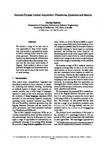
Figure 1: Different modes of visualization. In the traditional mode of visualization at left, the solver dumps all data to disk. Many insitu visualization projects couple the entire visualization within the solver and dump viewable images to disk, as shown in the middle. Although our coprocessing library supports this mode, we encourage the more versatile mode at right where the coprocessing extracts salient features and computes statistics on the data within the solver.

from disk storage is beginning to dominate the time spent in both the solver and the visualization [12]. Coprocessing can be an effective tool for alleviating the overhead for disk storage [22], and studies show that visualization algorithms, including rendering, can often be run efficiently on today’s supercomputers; the visualization requires only a fraction of the time required by the solver [24]. Whereas other previous work in visualization coprocessing completely couples the solver and visualization components, thereby creating a final visual representation, the coprocessing library provides a framework for the more general notion of salient data extraction. Rather than dump the raw data generated by the solver, in coprocessing we extract the information that is relevant for analysis, possibly transforming the data in the process. The extracted information has a small data representation, which can be written at a much higher fidelity than the original data, which in turn provides more information for analysis. This difference is demonstrated in Figure 1. A visual representation certainly could be one way to extract information, but there are numerous other ways to extract information. A simple means of extraction is to take subsets of the data such as slices or subvolumes. Other examples include creating isosurfaces, deriving statistical quantities, creating particle tracks, and identifying features. The choice and implementation of the extraction varies greatly with the problem, so it is important that our framework is flexible and expandable. The following sections describe the architecture of our framework and give numerous examples of how it can be used for analysis in different scientific domains. In the following sections we present the ParaView Coprocessing

Library. While the concept of in situ visualization is not new, we will show a number of design considerations we have made as part of the library to simplify the process of integrating coprocessing into a simulation code. We will also discuss some modifications we made to the ParaView application to simplify configuring and interacting with coprocessing. We will also show that, as a general purpose framework usable with a variety of simulations, the coprocessing library is scalable and runs efficiently on modern high performance computing (HPC) clusters. 2

P REVIOUS W ORK

The concept of running a visualization while the solver is running is not new. It is mentioned in the 1987 National Science Foundation Visualization in Scientific Computing workshop report [9], which is often attributed to launching the field of scientific visualization. Over the years, there have been many visualization systems built to run in tandem with simulation, often on supercomputing resources. Recent examples include a visualization and delivery system for hurricane prediction simulations [4] and a completely integrated meshing-to-visualization system for earthquake simulation [24]. These systems are typically lightweight and specialized to run a specific type of visualization under the given simulation framework. A general coupling system exists [5] which uses a framework called EPSN to connect M simulation nodes to N visualization nodes through a network layer. Our approach differs in that we link the codes and run on the simulation nodes, directly accessing the simulation data structures in memory. SCIRun [7] provides a general problem solving environment that contains general purpose visualization tools that are easily integrated with several solvers so long as they are also part of the SCIRun problem solving environment. Other more general purpose libraries exist that are designed to be integrated into a variety of solver frameworks such as pV3 [6] and RVSLIB [3]. However, these tools are focused on providing imagery results whereas in our experience it is often most useful to provide intermediate geometry or statistics during coprocessing rather than final imagery. Recent efforts are utilizing the largest supercomputing platforms to run visualization post-processing. These tools include ParaView [10], which provides the framework for our coprocessing, and VisIt [21]. Ultimately, the integration of coprocessing libraries into solvers gets around the issues involved with file I/O. There are also some related efforts in making the I/O interfaces abstract to allow loose coupling through file I/O to be directly coupled instead. Examples include the Interoperable Technologies for Advanced Petascale Simulations (ITAPS) mesh interface [1] and the Adaptable I/O System (ADIOS) [8]. If these systems become widely adopted, then it could simplify the integration of coprocessing libraries with multiple solvers. 3

T HE PARAV IEW C OPROCESSING L IBRARY D ESIGN

The ParaView Coprocessing Library is a C++ library with an externally facing API to C, FORTRAN and Python. It is built atop the Visualization Toolkit (VTK) [17] and ParaView [18]. By building the coprocessing library with VTK, it can access a large number of algorithms including writers for I/O, rendering algorithms, and processing algorithms such as isosurface extraction, slicing, and flow particle tracking. The coprocessing library uses ParaView as the control structure for its pipeline. Although it is possible to construct pipelines entirely in C++, the ParaView control structure allows pipelines configured through Python scripts and pipelines connected remotely, either through a separate cluster or directly to an interactive visualization client running on an analyst’s desktop machine. Since the coprocessing library will extend a variety of existing simulation codes, we cannot expect its API to easily and efficiently

Figure 2: The ParaView Coprocessing Library generalizes to many possible simulations, by means of adaptors. These are small pieces of code that translate data structures in the simulation’s memory into data structures the library can process natively. In many cases, this can be handled via a shallow copy of array pointers, but in other cases it must perform a deep copy of the data.

process internal structures in all possible codes. Our solution is to rely on adaptors, Figure 2, which are small pieces of code written for each new linked simulation, to translate data structures between the simulation’s code and the coprocessing library’s VTK-based architecture. An adaptor is responsible for two categories of input information: simulation data (simulation time, time step, grid, and fields) and temporal data, i.e., when the visualization and coprocessing pipeline should execute. To do this effectively, the coprocessing library requires that the simulation code invoke the adaptor at regular intervals. To maintain efficiency when control is passed, the adaptor queries the coprocessor to determine whether coprocessing should be performed and what information is required to do the processing. If coprocessing is not needed, it will return control immediately to the simulation. If coprocessing is needed, then the coprocessor will specify which fields (e.g., temperature, velocity) are required of the adaptor to complete the coprocessing. Then the adaptor passes this information and execution control to the coprocessing library’s pipeline. 3.1

Adaptor Design

One of the principle challenges in converting data from a running simulation is that of memory management [22]. In many cases, a job request is sized to fit either a time bound, that is number of machines needed to process fast enough for some real-time need, or a memory bound, that is enough machines with enough total memory to fit all the data. In either case, there will always be a non-zero cost trade-off in terms of both time and memory when performing in situ analysis. The simplest answer to address resident memory and time increases caused by coprocessing is to use more machines than those required by the simulation alone. Of course, this may not always be possible and other options must be used in constructing the adaptor. When memory is a limited factor, the adaptor must use one of two solutions. The first option is to access the resident simulation memory directly using potentially complicated pointer manipulation, such as modified strides and non-standard ordering. This is the method we used to connect efficiently with CTH and will be discussed in more detail in Section 4. The second option uses a much smaller region of memory than normally required by carefully managing construction of analysis classes [23] or by streaming the data in smaller consumable sizes. If memory is not a limiting factor, the adaptor may deep copy the data from the simulation data structure into into a VTK data object. This comes at a cost of doubling the required resident storage. In

addition there is a CPU cost involved with copying the data, but it is paid once at the beginning of pipeline execution and the remaining pipeline’s algorithms can operate on that data. It is important to weigh this upfront CPU cost against the cost of stalled cycles while writing data to disk [22]. In both cases the same pipeline would be executed, but in the case where data is written to disk for postprocessing, not only must the data must be written to disk it must be later read from disk by the visualization tool to receive a final, fully processed result. 3.2 Pipeline Configuration Tools Coprocessing is essentially a batch task. It runs as part of the solver, most probably on a cluster or a supercomputer and has no user interface. Therefore, it needs to be configured before the solver is run. This configuration needs to specify at least the following. • What should be extracted and saved? Extracted data can be isosurfaces, particle traces, slices, etc. • What are the parameters for the extraction algorithms? Parameters can include isosurface values, particle tracker seeds, slice location, etc.

usual way [18], modifying any of the stand-in ranges as necessary to match the expected values in the final version. Finally, we export, using the coprocessing script plugin, to a configuration file that will include these modifications. 3.3

Interactive In Situ Visualization

Although we’ve worked to address the limitations that come with pre-configuring a pipeline, there may still be some unexpected mesh configurations or quantities that arise in the data over the course of a simulation’s run. To handle these last unknowns in the coprocessing library, we use a client-server mechanism to allow an interactive ParaView client to connect to a server running inside a coprocessing pipeline. We have modified the ParaView client application to allow it to read from a coprocessing data source in place of a file. Using this, an analyst can construct a pipeline interactively in the ParaView client via this live data source and can change algorithm parameters on-the-fly to accommodate unexpected situations. This does not yet allow modification of the pre-configured pipeline the coprocessing library has loaded, but this will be addressed in future versions of the system.

• When should the extracted data be saved? For example the extracted data could be saved every tenth simulation step or when the maximum speed exceeds a certain value. • On which part of the data should the algorithms be applied? For example, the algorithms could be run on all the data or a subset of the blocks determined by an identifier, by a region of space, or by more elaborate selection criteria such as those that have maximum speed larger than a threshold. To simplify this input configuration we leverage the ParaView control structure underneath the coprocessing library. We use Python scripting to specify an input configuration. While normally created using a text editor, this process can be difficult and error prone. It is much more convenient to visually position a slice plane than it is to enter a point and a normal. For example, in ParaView, the position and the orientation of a plane can be specified using a 3D widget. This widget allows interaction by dragging the plane back and forth and rotating it using the handles of the direction arrow. Based on conversations with collaborators, we believe that most analysts prefer to interact with a graphical user interface than to manually code a coprocessing pipeline. To address this, we extended ParaView with a plugin that enables it to write pipelines as coprocessing scripts. An analyst can interactively create a pipeline and then write it out as a Python script, which can be read later by the coprocessing library when the simulation is running. A major difficulty in developing such a user interface for configuration is that when an analyst uses coprocessing, unlike postprocessing, most of the information about the problem is not available. For example, an initial mesh may be available, but if, during the simulation run, the mesh is modified based on deformation (e.g., in fluid-solid mechanics) pipelines constructed taking into account only the initial mesh may become quickly invalid. As another example, without the knowledge of the full range quantities take during a run, how do we present a tool from which a user can select valid values? In order to address this limitation, we’ve modified ParaView to allow analysts to modify the ranges in any existing data. Thus we start by working from an existing simulation output. This may be either a similar problem or a less refined version of the goal problem that approximately matches the expected bounds and variable ranges of the final version we wish to run. We then load this similar output into ParaView and interactively construct a pipeline in the

Figure 3: By allowing client-server connections to the coprocessing pipeline, we can export partially processed data to a smaller, specialized visualization cluster where some visualization algorithms perform more efficiently. In this way, ParaView’s coprocessing makes the most efficient use of all available resources.

As an added benefit of enabling the client-server architecture in the library, we can offload some or all of the visualization and analysis pipeline to a separate machine, e.g., a smaller visualization cluster with specialized graphics hardware (see Figure 3). Although the algorithms discussed in Section 4 are scalable to large HPC clusters, not all algorithms in the visualization pipeline will scale as efficiently as the simulation, which limits the effectiveness of direct coupling. In this situation we can funnel the data to a smaller cluster with more memory to handle the visualization task. Instead of a memory-to-memory copy, the tradeoff becomes a copy at network speed. However, network speeds are still generally much faster than writing data to, and later reading it from, disk. Finally, by decoupling some of the algorithms from the main computation, we can connect, disconnect, and modify them at will, much like the interactive client, without interfering with the simulation’s performance. 4

R ESULTS

The ParaView Coprocessing Library is designed to be general purpose. That is, it is intended to be integrated into a variety of solvers and used in multiple problem domains. First, we demonstrate the general scalability of the framework. Then, we will look at specific results coupling with simulations. 4.1

Algorithm Performance

In order to test general framework performance, we look at two commonly used ParaView algorithms, Slice and Decimate. We also take a look at corresponding file writes of the algorithms’ outputs.

0.1  0.09  Slice Time (sec) 

0.08 

20  18  Slice Write Time (sec) 

While the output size from Slice and Decimate will be significantly smaller, therefore writing out much faster, than the original input mesh, this gives us an opportunity to look at what impact, if any, the framework’s file representation has on scalability.

0.07 

16  14  12  10  8  6  4  2 

0.06 

0 

0.05 

0 

0.04 

5000 

10000 

15000 

20000 

25000 

30000 

35000 

25000 

30000 

35000 

Cores 

0.03  0.02  14 

0  0 

5000 

10000 

15000 

20000 

25000 

30000 

35000 

Cores  0.5  Decimate Time (sec) 

0.45  0.4  0.35 

Decimate Write Time (sec) 

0.01 

0.3 

12  10  8  6  4  2  0 

0.25 

0 

0.2 

5000 

10000 

15000 

20000 

Cores 

0.15  0.1  0.05  0  0 

5000 

10000 

15000 

20000 

25000 

30000 

35000 

Figure 5: Time to write slices (top) and decimated geometry (bottom) extracted from PHASTA data.

Cores 

4.2.1 Figure 4: Running time of extracting slices (top) and decimating geometry (bottom) from PHASTA data. The dashed lines indicate perfect scaling.

The running time for the two algorithms are shown in Figure 4. These curves are from a strong scaling study where the size of the input mesh does not change with the quantity of cores. The red dashed line in the images represents optimal scaling. As expected with strong scaling, the time converges to a minimum running time. The curves of Slice and Decimate follow the same trajectory as the optimal curve and both are only marginally less efficient than optimal. The time to write for each of the two algorithms is shown in Figure 5. In this case the expected optimal performance is not shown, but would be drawn as a horizontal line incident with the first point. The optimal line is flat for file I/O because although we are increasing the amount of computing resources, we are using the same amount of file I/O resources each time, for a given mesh size. However, despite the optimal line being flat, there is some overhead in our implementation due to communication before writing to disk. The variance in the write times is due to contention with other jobs running on the cluster writing out to the same shared I/O resource. Although the performance of the write is not bad, it grows slower than linear with the number of cores, it is not optimal. We are continuing to investigate more efficient methods for writing results. 4.2

Simulation Coupling

We present three simulation codes, Phasta, CTH and S3D, that we have connected with the library and the results of running with these systems.

Phasta

PHASTA is a Parallel, Hierarchic (2nd to 5th order accurate), Adaptive, Stabilized (finite-element) Transient Analysis tool for the solution of compressible or incompressible flows. Typical applications not only involve complicated geometries (such as detailed aerospace configurations) but also complex physics (such as fluid turbulence or multi-phase interactions). PHASTA [25] has been shown to be an effective tool using implicit techniques for bridging a broad range of time and length scales using anisotropic adaptive algorithms [14] along with advanced numerical models of fluid turbulence [19, 20]. Even though PHASTA uses implicit time integration and unstructured grids, it demonstrates strong scaling on the largest available supercomputers [16, 13] where a 512 fold increase (9 processor doublings) yielded a 424 fold time compression on a fixed mesh. Although weak scaling applications can double the mesh size with each processor doubling to bring ever more detailed resolution in finite time, in this paper we push PHASTA’s strong scaling ability to compress time-to-solution so as to evaluate the ParaView co-processor’s ability to provide a live view of an ongoing simulation near PHASTA’s strong scaling limit. The application involves simulation of flow over a full wing where a synthetic jet [15] issues an unsteady crossflow jet at 1750 Hz. One frame of this live simulation is shown in Figure 6 where two different filter pipelines have been evaluated in two separate runs of PHASTA. The mesh for these runs used 22M tetrahedral elements to discretize the fluid domain. The flow was solved on 16k (16,384) cores of IBM BG/P at the Argonne Leadership Computing Facility. This facility has a high speed network to up to 100 visualization nodes, which share 200 GPUs (e.g, 25 Nvidia S4s). For this study we varied the number of visualization nodes to evaluate the co-processing libraries ability to provide a live view of the ongoing flow simulation and to evalu-

Figure 6: Isosurface of vertical velocity colored by speed and cut plane through the synthetic jet (both on 22 Million element mesh).

ate the tax levied on the flow solver. The motivation for this study is based on our ongoing development of a computational steering capability wherein we would like to iterate the key parameters of the flow control (e.g, the frequency, amplitude, location etc) guided by live visualization. In the studies below we consider the scenario with the highest stress on the co-processing library, where the filter pipeline is evaluated on every step. In this high time compression mode, the local mesh size on each processor is such that the flow solver uses a small fraction of available memory, allowing a data copy to be used for the most efficient in situ data extract process. The first filter pipeline that was evaluated was a slice that cuts through the synthetic jet cavity and the jet cross flow. As this plane is easily defined in advance of the simulation, it did not need to be altered while the simulation was ongoing so there was no live updating of the filter pipeline making every step very close to the same computational effort. The computational time was measured in several stages of the co-visualization process. The time spent in the flow solve was verified to be independent of the filter and averaged 0.895 s (seconds) per step. Since we would like to see every time step in this case, the simulation is blocked until the data extract is delivered to the co-processing nodes. For this filter pipeline the total blocked time was 0.125 s resulting in a 14.4% tax on the simulation. Further breaking down this tax, the key contributions are: the data copy (0.0022 s), filter execution (0.0066 s), aggregation (0.0053 s), transport via VTK sockets (0.0148 s), initialize pipeline (0.0620 s) and cleanup (0.0345 s). Note that the last two account for 75% of the time. Future developments that allow these two costs to be done only on the first and last step are straightforward and worthwhile for runs where the filter pipeline is not being altered throughout the simulation. With these two removed the tax of a slice visualization would be reduced to 3.6%, which is very small for such a worst cases scenario (visualize every step of a very fast simulation). Clearly if only every nviz steps were visualized this tax would be amortized across nviz steps. The aggregation time and the transport time show a significant dependance upon the number of sockets since this directly sets the number of levels that the data must be reduced and communicated on the BGP. By varying the number of sockets per pvserver, the aggregation time was able to be reduced substantially. Although this does result in more, smaller messages being sent over more sockets to a finite number of pvservers and ultimately an appending of the data onto the fixed number of pvservers, the penalty to these phases was small and more than offset by the reduction in aggregation time. The results described above were for 10 Eureka nodes running 20 pvservers and 16 sockets per pvserver (total of 320 sock-

ets). When only 10 pvservers were used with 10 nodes and 1 socket per pvserver (total of 10 sockets), the total blocking time increased 33%. If we again discount the setup and close time (which are unaffected) the increase is 236% (e.g. from 3.6% to 8.4%). A similar analysis on the contour filter shows similar trends on this somewhat heavier filter (e.g., the data extract of the contour averages 79.9 while the slice was 9.44 MB or 8.38 times as large). Here the current co-vis tax was 23.5%, which could be reduced to 8.86% with the elimination of setup and close costs. Again, the number of sockets played a large role increasing these taxes by 241% and 475%, respectively. Note that the appending phase on the pvserver is not blocking the solver application so long as the pvserver can append and render the data before the next time time step’s data arrives. Even this blocking could be removed by relaxing the constraint of a live visualization with tight synchronicity between the visualization and the solve but, since the goal is to demonstrate computational steering capability, this constraint is maintained in these studies. For the case just described, the pvserver is able to manage this constraint down to 2 pvservers running on 1 node with 2 sockets per pvserver. The contour begins to show some delay (not completing its rendering before the next data set arrived) in this configuration but is fine at the next, less stressful configuration of 5 pvservers, 5 nodes and 16 sockets per node. It is clear that live visualization of complex, unsteady simulations is possible with the in situ data extract capability provided by this co-processing library on currently available hardware. Larger full machine studies of the same process on meshes up to 3.2B elements are currently underway [11]. 4.2.2

CTH

CTH is an Eulerian shock physics code that uses an adaptive mesh refinement (AMR) data model. We examine a simulation of an exploding pipe bomb shown in Figure 7. Using an algorithm that finds water-tight fragment isosurfaces over each material volume fraction within the AMR cells, we can find fragments that separate from the original mesh and measure various quantities of interest in these fragments. The challenge in finding an isosurface over values in an AMR mesh is in the difference of resolution between cells. More so this difference can also bridge processor boundaries, requiring ghost cell information at two different resolutions. We handle this by finding connected neighbors using an all-to-all communication at the beginning of computation and then exchanging ghost data between only connected neighbors and finally perform the AMR corrected isosurface algorithm. The result is a polyhedral mesh surface

90 Refinement Depth 6 Refinement Depth 7

80

Seconds

70 60 50 40 30 20 10 0

5000

10000 15000 20000 25000 30000 35000 Cores

400 Refinement Depth 6 Refinement Depth 7

350

Figure 7: Fragments detected in a simulation of an exploding pipe.

Blocks per Core

300 250 200 150 100

that contains no gaps and can be significantly smaller than the original AMR mesh. In some cases, where an analyst is only concerned with a histogram of fragment quantities, the data written can be on the order of bytes. One other particular challenge associated with CTH is the memory layout. Although the blocks of data are represented sequentially, the multidimensional order is different from what is used in VTK. To address this, we developed an interface wrapper above the standard VTK array. The wrapper reimplements the array’s accessor functions to handle the order difference between the two architectures. Although more expensive (additional pointer arithmetic) than direct, iterable access to the data, it saves us from a memory copy. Analysts tend to run CTH at the upper edge of available memory, so deep copying is usually not an option. We ran this pipeline on the new ASC/NNSA machine Cielo using from 1 thousand to 32 thousand cores. To simplify the scaling process, we increase only the depth limit on mesh refinement to increase the size of the problem. By incrementing this parameter the mesh size increases by at most a factor of eight, but in practice increases less than eight due to CTH choosing not to refine certain regions. We run each depth as a strong scaling problem up until the number of blocks per core dropped below a minimum suggested by the simulation. We then increase the depth and rerun to larger scale until we are able to run on 32 thousand cores. The results of these runs are shown in Figure 8 with each refinement depth represented as a separate line. The sizes in number of blocks resulting from these refinement levels are also shown. Although this algorithm works well enough to achieve a high number of communicating cores, as is visible in Figure 8 it is no longer performing any speedup beyond 16 thousand processors. This does not diminish overall speedup of the run when measured in combination with the simulation, and, more importantly, it is still much faster than writing the full dataset to disk, but there is room for increased efficiency. For instance, the all-to-all calculation is performed at each iteration of coprocessing pipeline and could be cached for a given configuration of AMR blocks, such that it would only need to be recomputed when the AMR hierarchy is redefined. Because much of this same connectivity information

50 0 0

5000

10000 15000 20000 25000 30000 35000 Cores

Figure 8: Fragment detection algorithm’s scaling results on a set of different refinement depths. Each line represents one depth run for a set of core counts corresponding to one problem size. The first image shows running time. The second image shows the corresponding blocks per processor at each refinement.

is already available and used by the simulation code, it may be possible to expose this information to the fragment detection algorithm so that the all-to-all communication is not necessary at all. 4.2.3

S3D

Another application of interest is S3D, which simulates turbulent reacting flows. S3D is used to simulate, for example, fuels burning in high-speed flows, which provides vital insight for improving the efficiency of automobile engines. Figure 9 shows analysis performed in situ as an attempt to characterize autoignition: principal component analysis (PCA) is run on 8 × 8 × 8 blocks of the simulation to determine which species concentrations are correlated to others inside each block. This results in a number of eigenvalues and eigenvectors for each block as illustrated in Figures 9 and 10. The eigenvalues indicate the importance of the correlation whereas the eigenvectors identify the tendency of each species to participate in the associated reaction mode exhibited in the block. If we wrote out the eigenvalues and eigenvectors instead of raw simulation results, we could save approximately 95% of the disk bandwidth per checkpoint. However, because low eigenvalues represent uninteresting or non-physical reaction modes, we need not write them. Figure 11 shows how eigenvalue magnitude varies as the index of the eigenvalue is increased. Only the first few eigenvectors in any block are likely to be of interest, which has the potential of saving an additional 80% of the disk bandwidth. Furthermore, it

The next step is to allow the user to analyze the simulation data while the simulation is running. This will be done by using ParaView’s client/server architecture to stream results from the machine the simulation is running on to a machine that is more conveniently available for actual viewing. ACKNOWLEDGEMENTS Sandia is a multiprogram laboratory operated by Sandia Corporation, a Lockheed Martin Company, for the United States Department of Energy’s National Nuclear Security Administration under contract DE-AC04-94AL85000. R EFERENCES

Figure 9: Demonstration of PCA on a reduced-resolution subset of a lifted ethylene jet simulation. On the left is the concentration of one chemical species. To the right is a PCA of 8×8×8 sub-blocks colored by the magnitude of index-0 eigenvalue. Low eigenvalue magnitudes indicate regions that might be discarded to reduce disk bandwidth.

Figure 10: Eigenvalue magnitudes from PCA of the full-resolution (2025 × 1600 × 400) simulation, computed on 1,500 processes. Autoignition occurs about midway up the simulated domain.

helps to identify which blocks are of interest and which are not so that we might save raw simulation data in regions of interest. Figure 11: Plot of the maximum of the ith eigenvalue magnitude over the entire domain vs. i. We see how only the first few eigenvectors are of interest, resulting in a large potential savings of disk bandwidth.

5

C ONCLUSION

Writing, reading, and analyzing simulation results can take an inordinate amount of time by conventional means. In these cases, coprocessing should be considered. Not only can the coprocessing computations be done on machines that are powerful enough, the savings in file I/O and data management are a big benefit as well. Perhaps the biggest improvement can be achieved on analyzing time dependent results such as particle tracking. With coprocessing, the necessary accuracy can be obtained while avoiding writing the simulation data out every time step. Note that our results compare coprocessing time to the time it takes the solver to perform one time step. However, in general this is usually not necessary and often undesired; the small delta change in fields is required for accurate solving but only yields interesting results after several iterations.

[1] K. Chand, B. Fix, T. Dahlgren, L. F. Diachin, X. Li, C. Ollivier-Gooch, E. S. Seol, M. S. Shephard, T. Tautges, and H. Trease. The ITAPS iMesh interface. Technical Report Version 0.7, U. S. Department of Energy: Science Discovery through Advanced Computing (SciDAC), 2007. [2] H. Childs. Architectural challenges and solutions for petascale postprocessing. Journal of Physics: Conference Series, 78(012012), 2007. DOI=10.1088/1742-6596/78/1/012012. [3] S. Doi, T. Takei, and H. Matsumoto. Experiences in large-scale volume data visualization with RVSLIB. Computer Graphics, 35(2), May 2001. [4] D. Ellsworth, B. Green, C. Henze, P. Moran, and T. Sandstrom. Concurrent visualization in a production supercomputing environment. IEEE Transactions on Visualization and Computer Graphics, 12(5), September/October 2006. [5] A. Esnard, N. Richart, and O. Coulaud. A Steering Environment for Online Parallel Visualization of Legacy Parallel Simulations. In Proceedings of the 10th International Symposium on Distributed Simulation and Real-Time Applications (DS-RT 2006), pages 7–14, Torremolinos, Malaga, Spain, October 2006. IEEE Press. [6] R. Haimes and D. E. Edwards. Visualization in a parallel processing environment. In Proceedings of the 35th AIAA Aerospace Sciences Meeting, number AIAA Paper 97-0348, January 1997. [7] C. Johnson, S. Parker, C. Hansen, G. Kindlmann, and Y. Livnat. Interactive simulation and visualization. IEEE Computer, 32(12):59–65, December 1999. [8] J. F. Lofstead, S. Klasky, K. Schwan, N. Podhorszki, and C. Jin. Flexible IO and integration for scientific codes through the adaptable IO system (ADIOS). In Proceedings of the 6th International Workshop on Challenges of Large Applications in Distributed Environments, pages 15–24, 2008. [9] B. H. McCormick, T. A. DeFanti, and M. D. Brown, editors. Visualization in Scientific Computing (special issue of Computer Graphics), volume 21. ACM, 1987. [10] K. Moreland, D. Rogers, J. Greenfield, B. Geveci, P. Marion, A. Neundorf, and K. Eschenberg. Large scale visualization on the Cray XT3 using ParaView. In Cray User Group, May 2008. [11] M. Rasquin, P. Marion, V. Vishwanath, M. Hereld, R. Loy, B. Matthews, M. Zhou, M. Shephard, O. Sahni, and K. Jansen. Covisualization and in situ data extracts from unstructured grid CFD at 160k cores. In Proceedings of the SC11, submitted, 2011. [12] R. B. Ross, T. Peterka, H.-W. Shen, Y. Hong, K.-L. Ma, H. Yu, and K. Moreland. Visualization and parallel I/O at extreme scale. Journal of Physics: Conference Series, 125(012099), 2008. DOI=10.1088/1742-6596/125/1/012099. [13] O. Sahni, C. Carothers, M. Shephard, and K. Jansen. Strong scaling analysis of an unstructured, implicit solver on massively parallel systems. Scientific Programming, 17:261–274, 2009. [14] O. Sahni, K. Jansen, M. Shephard, C. Taylor, and M. Beall. Adaptive boundary layer meshing for viscous flow simulations. Engng. with Comp., 24(3):267–285, 2008. [15] O. Sahni, J. Wood, K. Jansen, and M. Amitay. 3-d interactions between finite-span synthetic jet and cross flow at a low reynolds number and angle of attack. Journal of Fluid Mechanics, 671:254, 2011. [16] O. Sahni, M. Zhou, M. Shephard, and K. Jansen. Scalable implicit finite element solver for massively parallel processing with demon-

[17]

[18] [19]

[20]

[21] [22]

[23]

[24]

[25]

stration to 160k cores. In Proceedings of the SC09, Springer, Berlin, 2009. W. Schroeder, K. Martin, and B. Lorensen. The Visualization Toolkit: An Object Oriented Approach to 3D Graphics. Kitware Inc., fourth edition, 2004. ISBN 1-930934-19-X. A. H. Squillacote. The ParaView Guide: A Parallel Visualization Application. Kitware Inc., 2007. ISBN 1-930934-21-1. A. E. Tejada-Mart´ınez and K. E. Jansen. A dynamic Smagorinsky model with dynamic determination of the filter width ratio. Physics of Fluids, 16:2514–2528, 2004. A. E. Tejada-Mart´ınez and K. E. Jansen. A parameter-free dynamic subgrid-scale model for large-eddy simulation. Comp. Meth. Appl. Mech. Engng., 195:2919–2938, 2006. K. Thomas. Porting of VisIt parallel visualization tool to the Cray XT3 system. In Cray User Group, May 2007. D. Thompson, N. D. Fabian, K. D. Moreland, and L. G. Ice. Design issues for performing in situ analysis of simulation data. Technical Report SAND2009-2014, Sandia National Laboratories, 2009. D. Thompson, R. W. Grout, N. D. Fabian, and J. C. Bennett. Detecting combustion and flow features in situ using principal component analysis. Technical Report SAND2009-2017, Sandia National Laboratories, 2009. T. Tu, H. Yu, L. Ramirez-Guzman, J. Bielak, O. Ghattas, K.-L. Ma, and D. R. O’Hallaron. From mesh generation to scientific visualization: An end-to-end approach to parallel supercomputing. In Proceedings of the 2006 ACM/IEEE conference on Supercomputing, 2006. C. H. Whiting and K. E. Jansen. A stabilized finite element method for the incompressible Navier-Stokes equations using a hierarchical basis. International Journal of Numerical Methods in Fluids, 35:93– 116, 2001.