A Scalable Grid Scheduler for Real-Time Applications - UT Dallas

IJCA, Vol. 16, No. 1, March 2009

1

A Scalable Grid Scheduler for Real-Time Applications Cong Liu* and Sanjeev Baskiyar* Auburn University, Auburn, AL, 36849, USA.

Abstract In a grid computing environment, dynamicity and geographically distributed sites, make task scheduling problems challenging to solve. It is hard for a site to obtain precise real-time information about other sites whose load and computing resources may change dynamically. Moreover, the large number of individual resources of grid platforms raises scalability issues. Furthermore, many large scale data intensive applications make scheduling even more challenging since data transfer cost resources must be taken into consideration. In this paper we propose an innovative Peer-to-Peer Grid Scheduler (P2PGS) to solve such problems. P2PGS introduces two-phase scheduling framework that considers the large scale nature of the grid environment. P2PGS is composed of two phases: scheduling and dispatching. P2PGS is distributed and thus scalable since schedulers are distributed among resource sites. The scheduler at each site only needs the basic information of its neighbors to make dispatching decisions. Simulation results show that P2PGS can successfully schedule approximately 90 percent of computation-intensive tasks. For other tasks such as tasks with large data sets, it can successfully schedule more than 75 percent of them. Key Words: Grid computing, peer-to-peer scheduler, distributed scheduling, scalability, data transfer delay. 1 Introduction An emerging trend in computing is to use distributed heterogeneous computing systems constructed of networked machines. This trend has made possible the aggregation of geographically dispersed resources for the execution of largescale resource-intensive applications [3, 4]. Over the past years grid infrastructures have been deployed at larger and larger scales, with deployments incorporating tens of thousands of resources. This volume of resources raises scalability issues (e.g., resource discovery and monitoring). When considering the scheduling problem in grid systems, it is

vital for the scheduling algorithm to be scalable. In a Grid, resources are geographically distributed in multiple domains. Not only the computational and storage resources, but also the underlying networks connecting them are heterogeneous. Such heterogeneity results in different capabilities of task processing and data access. Traditional cluster systems normally contain a number of computing resources at the same location. So the time for data transmission was ignored. However, in a grid computing environment, for data-intensive tasks it is important to consider data transfer cost when making scheduling decisions [11], since the bandwidth between two geographically distributed sites may be slow and unstable. In this paper we propose an innovative Peer-To-Peer Grid Scheduler (P2PGS) that considers both the amount of computational resources and the data transfer. We consider the environment of multiple independent tasks arriving at geographically distributed sites. At each site the scheduler first schedules incoming tasks onto available resources. Those tasks that cannot be scheduled at the local site are dispatched to neighboring sites. Then a fine scheduling can be made by the schedulers located at corresponding neighboring sites in a better way since they have better real-time information of the local resources. Thus P2PGS is highly distributed; it can run on each site where it just needs to know the basic information of its immediate neighboring sites. P2PGS finds each site’s favorite neighbors using the connectivity bandwidth and computing capacities. Our peer-to-peer scheduling strategy has the following advantages. First it does not need to know the global state of the grid. Second the local scheduler can utilize real-time and precise information such as information from a local load forecaster to make adaptive decisions. The outline of the paper is as follows. Section 2 contains related work in the area of grid scheduling. The target grid has been detailed in Section 3. Section 4 describes the proposed scheduling and computing model. Section 5 introduces our scheduling algorithm. Simulation details and performance analysis are discussed in Section 6. The summary and directions for future work are given in Section 7. 2 Related Work

*

Computer Science and Software Engineering. {liucong, baskisa}@auburn.edu.

E-mail:

Most previous works only considered the computation time of the execution of a task, but omitted the transmission time of

ISCA Copyright© 2009

IJCA, Vol. 16, No. 1, March 2009

2

data, which, as stated above, could be significant in real world applications. In the Grid, a task may be dispatched to a remote site to be executed, so that the cost of transferring the task’s data might vary according to the link condition. Furthermore, previous works assume that each site has precise information about all other sites in a grid, which has a large overhead and is difficult to obtain. Casanova et al. [2] describe an adaptive scheduling algorithm for parameter sweep applications such as drug design [1] in Grid environments that takes data transfer issues into consideration. However, they make scheduling decisions centrally, assuming full knowledge of current loads, network conditions and topology of all sites in the grid. Other efforts have tried to address the problem of data management services and efficient data transmission protocols. For example, in the Globus project [5], a data transport protocol called GridFTP [6] efficiently solves the problem of data transmission. Also, basic cost models for analyzing replicated and geographically distributed data have been described. The Network Weather Service (NWS) [13] has also been developed as an efficient method of measuring and forecasting a network’s bandwidth. Ranganathan and Foster [12] consider dynamic task scheduling along with data transfer requirement. Data replication is used to reduce communication bandwidth consumption and avoid data access hotspots. Also, computation scheduling and data replication strategies are partly independent of one another. Park et al.[10] describe a scheduling model that considers both the amount of computational resources and data availability in a data grid environment. However, assigning a task to the machine that has the fastest execution time may result in poor performance due to the cost of retrieving the required input data from data repositories. They have not addressed the problem of optimizing the selection of a destination site. Moreover, the key limitation of these approaches is that they are not scalable since they assume that the centralized scheduler has the full knowledge of grid resources. Several effective scheduling algorithms such as Earliest Deadline First (EDF) [11], Sufferage [12], and Min-Min [13] have been proposed in previous works. The EDF algorithm basically schedules tasks with the shortest deadlines first. The rationale behind Sufferage is to allocate a site to a task that would “suffer” most in completion time if the task is not allocated to that site. For each task, its sufferage value is defined as the difference between its best minimum completion time and its second-best minimum completion time. By doing so, this algorithm always assigns a task with the largest sufferage value first to the computing resource that gives the minimum completion time. The complexity of the conventional Sufferage algorithm, which is applied to a single cluster system, is O(mn2), where m is the total number of machines and n is the number of incoming tasks. If Sufferage is applied in a multi-cluster based grid system, it complexity becomes O(msn2) where s is the number of clusters within the grid. The Min-Min heuristic begins with computing the set of minimum completion time for each task on all machines. Among all tasks, the one that has the overall minimum

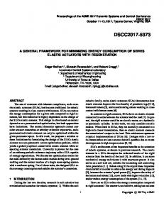
completion time is chosen and allocated to the tagged resource. The goal of Min-Min is to attempt to complete as many tasks as possible. The complexity of Min-Min algorithms is O(msn2), if applied in a grid system. This paper introduces a peer-to-peer scheduling framework and a scalable dispatching strategy for selecting the best remote site to assign tasks. We introduce a look-ahead strategy that searches more than one hop throughout the grid to get better performance. We use mobile tickets to route results of computation through the network, to schedule tasks in the network. 3 System Model In our grid model sites interconnect through WAN as shown in Figure 1. We define a site as a location that contains many computing resources of different processing capabilities. At each site, there is one main server and several supplemental servers, which are in charge of collecting information from all machines within that site. If the main server fails, a supplemental server will take over. Intra-site communication cost is usually negligible as compared to inter-site communication. Super Computer

Servers

PC

PC

PC

WAN

PC

WAN

PC Servers Server Enterprise Server Server

WAN

Server

Super Computer

Forwarded Tasks Incoming Tasks

Server

Outgoing Scheduler

Server Locally unschedulable tasks

Computing Resources

Local Scheduler

local site

Figure 1: Grid model Given that each site will have different number and types of computers, the general computing capacity of each site can vary significantly. We classify computers into three categories: personal computers, servers, and supercomputers. A national laboratory or a big university may have supercomputers, whereas small companies and individual users have only servers or personal computers. In Figure 1, we use a

IJCA, Vol. 16, No. 1, March 2009

triangle to represent a site with personal computers, circles to represent a site with servers, and squares to represent a site with supercomputers. 4 Scheduling Algorithm We address the problem of scheduling a bag of independent tasks, with deadline constraints, on the grid. Since some of these tasks may be large and cannot be completed within deadline at local site, our algorithm attempts to find a more powerful remote computing resource in the grid. P2PGS consists of two phases. First incoming tasks at each site are ranked and assigned to specific resources on a site according to several different strategies. Second those tasks that are unable to be scheduled are dispatched to remote sites where the same scheduling algorithm is used to make scheduling decisions. The pseudo code of P2PGS is shown in Figure 2. P2PGS // Q is a task queue in site S Sort Q by increasing deadline Schedule if unscheduled tasks remain in Q Dispatch endif end P2PGS Figure 2: P2PGS main function 4.1 Notations A real-time task has a deadline, instructions, input data, and output data. To each task we assign a ticket, which contains its attributes. A ticket has several fields: task ID, valid/invalid, instruction size, input data size, output data size, estimated minimum completion time and route information. If the site at which the task ti arrives is unable to meet ti’ deadline, it forwards ti to its neighbor. Each task’s ticket will be sent to remote sites to make scheduling decisions, instead of the task itself. The main server at each site will receive tickets collected from other sites and process them to make scheduling decisions. When a task can be executed at a remote site within its deadline, the ticket will be marked valid and the destination site will be recorded. Tickets are forwarded depending upon the computing capacity of sites, network bandwidth. For every site, we rank its neighbors using bandwidth and neighbors’ computing capacity, and the one with the highest rank will be chosen as the best neighbor. Tickets are forwarded to the best neighbor first. Also, we define a variable “depth” that is the amount of look-ahead depth in the network. For every site, periodically (say every hour) the neighbor list is updated. We assume that the transmission time of a ticket can be ignored since its size is very small. We also assume that the estimated size of output data can be estimated; and in each local site, communication time can be ignored. Below are the mathematic notations used in this paper:

3

• • • • • • • • • • • •

eij: Expected execution time of taski at sitej cijk: Expected transmission time of taski from sitej to sitek bij: Expected bandwidth between sitei and sitej sii: Size of input data of taski sio: Size of output data of taski sic: Size of code of taski, in terms of MI (Million Instruction) di: Deadline of taski cjk: Computing capacity of machinek at sitej, in terms of MIPS (Million Instruction Per Second) tij: Completion time for taski first situated at sitej ectim: The estimated minimum completion time for taski at sitem MCTij: The minimum estimated completion time for taski if executed on sitej sci: The general computing capacity of sitei

4.2 Computing Model A task’s completion time consists of two parts: data transfer time and execution time. tij = cijk + eij We need a different equation to adapt to different situations, as we introduce the look-ahead strategy which searches more than one hop in the grid to find a resource site to schedule tasks which cannot be finished within deadline at their local site. If the site is able to execute the task within the deadline, the completion time will be tij = sic / cjk However, if the task is forwarded to a neighbor sitej, then the estimated completion time of taski on machinek at sitej will be the sum of transmission and execution time. tij = ( sii + sio + sic)/ bij + sic / cjk 4.3 Scheduling At each site, various users may submit a number of tasks with different deadlines. The scheduler at each site puts all incoming tasks into a task queue. Tasks are sorted by increasing deadline so that the most urgent tasks can be scheduled first. Each task is scheduled on the machine that provides the minimum completion time. The pseudo code of the scheduling function is shown in Figure 3. 4.4 Dispatching If a task ti cannot be scheduled at its local site it is forwarded to the external scheduler which tries to find a remote site to schedule the task. In dispatching, previous works have selected a remote site randomly or used a single

IJCA, Vol. 16, No. 1, March 2009

4

Schedule for each unscheduled task t ∈ Q for each machine m ∈ S //visit in random order to balance load Compute estimated completion time for t on m endfor Let machine M provide the minimum completion time MCTt for t if MCTt < Dt // Dt is the deadline of t Schedule t on M Mark t scheduled Update count of unscheduled tasks in Q endif endfor end Schedule Figure 3: Schedule characteristic, such as computing capacity, bandwidth, or load. P2PGS uses both the computing capacity and bandwidth in dispatching. Furthermore, P2PGS helps decrease communication overhead since each site only needs to maintain its immediate neighbors’ basic information such as bandwidth and general computing capacity. The general computing capacity of a site is defined by its computing capacity category. Resource sites within a grid are categorized into three types: site with supercomputers, site with servers, and site with personal computer. A value of 3 is assigned to the general computing capacity of a site with supercomputers, while a value of 2 is assigned to the general computing capacity of a site with servers, and a value of 1 is assigned to the general computing capacity of a site with personal computers. The general computing capacity is used when selecting the best neighboring site in dispatching. For the purpose of forwarding a task, sites are ranked in decreasing order based on the value of bandwidth times general computing capacity, called HRF (Highest Rank First). The rank of neighbor j of sitei is defined as:

mark task i as un-schedulable and start processing the next task. The pseudo code of the dispatching function is shown in Figure 4.

Rankij = bij * scj

We generated eight sites with each site having a random number of computers between 20 and 50. The Communication to Computation Ratio (CCR) value of each task was varied between 0.01-1. We varied other parameters to understand their impact on different algorithms. The maximum value of depth is set to 3, which equals the maximum number of hops among neighbors according to our grid topology. The deadlines and number of tasks were chosen such that the grid system is close to its breaking point where tasks start to miss deadlines.

The external scheduler at first sends the ticket of ti to the best neighboring site sk to compute the estimated minimum completion time, emctim. After visiting a remote site, the value of depth is reduced by one. If depth is not 0, this neighboring site will choose its best neighbor and forward the ticket appropriately. According to the definition of depth, its value should equal the number of remote sites to which the ticket may be forwarded. After accumulating the estimated shortest completion time on all visited sites, we send task i to the remote site m that provides the minimum emctim, if ectim is less than di. If emctim is still greater than di, we re-send ti’s ticket to the second best neighboring site using the same strategy. This process continues until we can find a site to complete task i by the deadline. Basically our searching strategy is similar to the depth-first search. Finally, if we cannot find a remote site, we

5 Simulation and Analysis We have constructed a simulator to simulate the algorithm. Results of the experiments are analyzed and performance of the scheduler is evaluated. 5.1 Simulation Initialization We varied the instruction size, size of input and output datasets, bandwidth between sites, and each machine’s processing capability. The Successful Schedulable Ratio (SSR) has been used as the main metrics of evaluation. It is defined as:

SSR =

number of tasks meeting deadlines total number of tasks

5.2 Performance for Different Algorithms The first experiment set was to evaluate the performance using different algorithms. We use FCFS, EDF, Min-Min and Sufferage heuristics to rank tasks in each site’s local queue. HRF is used as the remote site chosen strategy. We set different values of depth to see which heuristic gives good and

IJCA, Vol. 16, No. 1, March 2009

5

Dispatch for each unscheduled task t ∈ Q while t is unscheduled && there is any neighbor remaining in S’s neighbor list while depth > 0 Compute MCTt,j on Sj which is ranked first in S’s neighbor list Remove Sj from the current base site’s neighbor list Depth-Find the highest ranked neighbor Sk of Sj, remove it from Sj’s neighbor list Let Sk be the current base site endwhile if Min{MCTt,i} < Dt Send t to the machine which provides Min{MCTt,i} Mark t as successfully scheduled endif endwhile if t is unscheduled Mark t as Un-Schedulable, and update S’s neighbor list endif endfor end Dispatch Figure 4: Dispatch 100%

FCFS EDF Min-Min Sufferage

80%

SSR

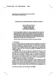
consistent performance. From Figure 5 we observe that all algorithms other than FCFS give roughly the same performance, though EDF outperforms a little bit when the number of tasks is less than 12,500 and Min-Min becomes the best one when number of tasks exceeds 12,500. When depth equals two, it is observed from Figure 6 that using EDF to rank tasks can get higher SSR than others. It is because our final criteria for judging whether a task can be scheduled or not is to compare the estimated minimal completion time with its deadline. Thus, scheduling those tasks with shorter deadlines first can make more tasks schedulable.

60%

40%

20% 5000

100%

FCFS EDF Min-Min Sufferage

SSR

80%

7500

10000

12500

15000

17500

20000

Number of Tasks

Figure 6: Performance comparison between different ranking algorithms when depth equals 2 60%

When depth equals three, the advantage of using EDF becomes more obvious, as shown in Figure 7. That’s because those tasks with short deadlines will be scheduled at first; while other ones with longer deadlines can wait some time to be scheduled on remote sites.

40%

20% 5000

7500

10000

12500

15000

17500

20000

Number of Tasks

Figure 5: Performance comparison between different ranking algorithms when depth equals 1

5.3 Performance for Different Remote Site Selection Strategy with Different Number of Tasks This experiment set was to evaluate the performance using different site selection strategies. We compare the

IJCA, Vol. 16, No. 1, March 2009

6

100%

HRF

100%

FCFS EDF Min-Min Sufferage

LCCF

Random

80%

SSR

SSR

80%

60% 40%

60%

20% 0%

40% 5000

7500

10000

12500

15000

17500

20000

5000

7500

Number of Tasks

10000

12500

15000

17500

20000

Number of Tasks

Figure 7: Performance comparison between different ranking algorithms when depth equals 3

Figure 9: Performance comparison using different searching strategies when depth equals 2

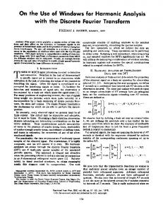
performance given by HRF against two other ranking methods Largest Computing Capacity First (LCCF) and Random. LCCF will first choose the neighboring site with the largest computing capacity; while Random just randomly selects one of the neighboring sites as the most favorite. We change the number of tasks and the value of depth to see which strategy gives the best and the most consistent performance. The value of CCR for each task is randomly chosen. We first set the value of depth to one. It is observed from Figure 8 that in general using HRF gives the best performance. In average HRF outperforms LCCF by 18 percent, and outperforms RC by 24 percent. The reason may be that HRF takes both computing capacity of neighboring sites and network bandwidth into consideration, which is more comprehensive than the other two.

When depth equals three, the same results come out, as we can see in Figure 10, although the percentage outperformed by HRF compared to the other two decreases very slightly.

HRF

100%

LCCF

Random

SSR

80% 60% 40% 20% 0% 5000

100%

HRF LCCF Random

SSR

80%

7500

10000 12500 15000 17500 20000

Number of Tasks

Figure 10: Performance comparison using different searching strategies when depth equals 3

60%

40%

5.4 Performance for Different Remote Site Selection Strategy with Different Depth

20% 0% 5000

7500

10000

12500

15000

17500

20000

Number of Tasks

Figure 8: Performance comparison using different searching strategies when depth equals 1 When we change the value of depth to two, it can be seen from Figure 9 that HRF still gives the best performance.

In this test, we want to evaluate performance by combing different site chosen strategies with different depth, for a fixed number of tasks, 15,000. From Figure 11 we find out that for all three strategies increasing depth can improve performance significantly. The achieved SSR by using HRF can reach above 90 percent when we increase the value of depth to 3, which is a very desirable performance. We argue that setting depth to the possible maximum value yields the best performance. Doing so may increase the possibility of finding remote sites that can meet tasks’ deadlines.

IJCA, Vol. 16, No. 1, March 2009

7

HRF

100%

LCCF

than the other two, as shown in Figure 13. The gap is not so obvious due to limited transmission possibilities because a task can be at most transmitted once from local site to a neighboring site.

Random

SSR

90% 100%

CCR=0.01 CCR=0.1 CCR=1

80% 80%

70% SSR

60%

60% 1

2

40%

3

Depth 20%

Figure 11: Performance comparison using different searching strategies combined with different depth

0% 5000

7500

5.5 Performance for Different Depths

Depth=1

Depth=2

Depth=3

15000

17500

20000

As Figure 14 shows, when we increase the depth to 2, the first case becomes much better in which instruction size is much larger than data size. 100%

CCR=0.01 CCR=0.1 CCR=1

80% 60%

40%

80%

SSR

12500

Figure 13: Performance for different CCR when depth equals 1

SSR

The second test was to evaluate the influence brought by searching different depths with a fixed CCR throughout the grid network. For all the remaining experiments we will choose EDF as our local queue ranking algorithm and HRF as site chosen strategy. From Figure 12 it can be seen that the grid scheduler gives much higher SSR by searching deeper through the grid network. By searching one more hop, performance improves by 40 percent. Another hop deep improves performance by another 15 percent. Thus, we can say that when incoming tasks are computation-intensive, searching deeper can significantly improve performance.

100%

10000

Number of Tasks

20%

60%

0% 5000

40%

7500

10000

12500

15000

17500

20000

Number of Tasks 20% 0% 5000

7500

10000

12500

15000

17500

20000

Number of Tasks

Figure 12: Performance comparison between different depths

Figure 14: Performance for different CCR when depth equals 2 When the depth increases to 3, such improvement becomes more significant, as shown in Figure 15. Thus, we can say that when incoming tasks are computation-intensive, searching deeper can significantly improve performance.

5.6 Performance for Different CCR 5.7 Performance for Different Depths with Different CCR In this experiment set we want to test the performance fluctuation by setting different instruction-data ratio for the same fixed depth. When grid scheduler only searches for neighboring sites (depth is one), the first case, in which instruction size is much larger than data size, is slightly better

In this test, we want to evaluate performance by combing different CCR with different depths, for a fixed number of incoming tasks, 15,000 tasks. From Figure 16 we find out that with fixed number of incoming tasks increasing depth can

IJCA, Vol. 16, No. 1, March 2009

8

CCR=0.01

CCR=0.1

specific information (such as computing capability of specific machines, each machine’s ready time, etc) to make adaptive decisions. We have conducted several experiments to evaluate the performance under different scenarios. Our scheduler is scalable and distributed. Each site only needs to know basic information of its neighboring sites. Simulation results show that P2PGS can successfully schedule approximately 90 percent of computation-intensive tasks. For other tasks such as tasks with large data sets, it can successfully schedule more than 75 percent of them. In the future we plan to make our scheduling algorithm more powerful to consider other factors that will affect the performance, such as fault tolerance and dynamicity of networks. Moreover, on the lower level, we plan to propose a local scheduling algorithm which better considers the characteristics of a grid environment.

CCR=1

100%

SSR

80% 60% 40% 20% 0% 5000

7500

10000

12500

15000

17500

20000

Number of Tasks

Figure 15: Performance for different CCR when depth equals 3

CCR=1

100%

CCR=0.1

CCR=0.01

SSR

90%

80%

70%

60% 1

2

3

Depth

Figure 16: Performance comparison using different depths combined with different CCR significantly increase the SSR when CCR equals 0.01 or 0.1. When CCR increases to 1, it can still achieve better performance, although not that significant. This is because transmission time will become longer, which makes remote computing resources less helpful. 6 Conclusion and Future Work In this paper we have proposed a real-time peer-to-peer grid scheduler that considers both the amount of computational resources and data transfer. Based on a standard grid model, we introduce the concept of peer-to-peer chosen strategy and look-ahead strategy. At the higher level, where fine global resource information is harder to obtain, it is easier for each local site to know the general information of its neighboring sites (such as load info, general computing capability and communication bandwidths of WAN links) to provide decentralized scheduling mechanisms. After choosing a neighboring site, it is easy for local scheduling to utilize more

References [1] R. Buyya, K. Branson, J. Giddy, and D. Abramson, “The Virtual Laboratory: Enabling Molecular Modeling for Drug Design on the World Wide Grid,” Technical Report CSSE-103 Monash University, 2001. [2] H. Casanova, G. Obertelli, F. Berman, and R. Wolski, “The AppLeS Parameter Sweep Template: User-Level Middleware for the Grid,” Proc. of Super Computing, November 2000. [3] A. Chervenak, I. Foster, C. Kesselman, C. Salisbury, and S. Tuecke, “The Data Grid: Towards an Architecture for the Distributed Management and Analysis of Large Scientific Datasets,” Journal of Network and Computer Applications, 23:187-200, July 2000. [4] I. Foster and C. Kesselman, The Grid: Blueprint for New Computing Infrastructure, Morgan Kaufmann, 1998. [5] The Globus Project [Online], Available: http://www.globus.org [Accessed May 8, 2007]. [6] W. Hoschek, J. Jaen-martinez, A. Samar, H. Stockinger, and K. Stockinger, “Data Management in an International Data Grid Project,” Proc. of the IEEE/ACM International Workshop on Grid Computing, pp. 77-90, December 2000. [7] C. Liu and J. Layland, “Scheduling Algorithms for Multiprogramming in a Hard Real-Time Environment,” Journal of the ACM, 20:46-61, January 1973. [8] M. Maheswaran, S. Ali, H. J. Siegel, D. Hensgen, and R. F. Freund, “Dynamic Matching and Scheduling of a Class of Independent Tasks onto Heterogeneous Computing Systems,” Proc. of the Heterogeneous Computing Workshop, pp. 33-40, April 1999. [9] D. Menasce, D. Saha, and S. Porto, “Static and Dynamic Processor Scheduling Disciplines in Heterogeneous Parallel Architectures,” Journal of Parallel and Distributed Computing, 28:1-18, July 1995. [10] S. M. Park and J.H. Kim, “Chameleon: A Resource Scheduler in A Data Grid Environment,” Proc. of the IEEE International Symposium on Cluster Computing & the Grid, pp. 258-265, May 2003.

IJCA, Vol. 16, No. 1, March 2009

9

[11] K. Ranganathan and I. Foster, “Decoupling Computation & Data Scheduling in Distributed Data-Intensive Applications,” Proc. of the IEEE International Symposium on High Performance Distributed Computing, pp. 352-361, July 2002. [12] K. Ranganathan and I. Foster, “Identifying Dynamic Replication Strategies for a High Performance Data Grid,” Proc. of the IEEE/ACM International Workshop on Grid Computing, pp. 75-86, November 2001.

[13] R. Wolski, N. Spring, and J. Hayes, “The Network Weather Service: A Distributed Resource Performance Forecasting Service for Meta-Computing,” Journal of Future Generation Computing Systems, 15:757-768, October 1999.

Cong Liu received the BE degree in Computer Science from Wuhan University of Technology, China in 2005. Currently he is a graduate student in the Department of Computer Science and Software Engineering at Auburn University, Auburn, AL. His research interests are in Task Scheduling on Large-scale Distributed Systems, and Packet Scheduling and Routing in Wireless Sensor Networks.

Sanjeev Baskiyar received the BS degree in Electronics and Communication Engineering from the Indian Institute of Science, Bangalore and the MSEE and PhD degrees from the University of Minnesota, Minneapolis. He also received the BS degree in Physics with honors and distinction in Mathematics. Currently, he is a tenured Associate Professor in the Department of Computer Science and Software Engineering at Auburn University, Auburn, AL. His experience includes industrial positions in Unisys Corporation and Tata Motors, India. He has made major research contributions in the areas of Scheduling, Computers, Computer Architecture and Real-time and Embedded Computing.