The test tries to establish the existence of a linear combination of the effect ...... Promela sources for the IBOC model that we use are freely available from URL.
A Scalable Incomplete Test for Message Buffer Overflow in Promela Models Stefan Leue, Richard Mayr, and Wei Wei Department of Computer Science Albert-Ludwigs-University Freiburg Georges-Koehler-Allee 51, D-79110 Freiburg, Germany E-mail: [leue|mayrri|wwei]@informatik.uni-freiburg.de
Abstract. In Promela, communication buffers are defined with a fixed length, and buffer overflows can be handled in two different ways: block the send statement or lose the message. Both solutions change the semantics of the system, compared to one with unbounded channels. The question arises, if such buffer overflows can ever occur in a given system and what buffer lengths are sufficient to avoid them. We describe a scalable incomplete boundedness test for the communication buffers in Promela models, which is based on overapproximation and static analysis. We first reduce Promela models to systems of communicating finite state machines (CFSMs) and then apply further abstractions that leave us with a system of linear inequalities. Those represent the message sending and receiving effect that the control flow cycles of every process have on any message buffer. The test tries to establish the existence of a linear combination of the effect vectors so that at least one message can occur an unbounded number of times. If no such linear combination exists then the system is bounded. We discuss the complexity of this test and present experimental results using our implementation in the IBOC system. Scalability of the test is in part due to the fact that it is polynomial for the type of sparse control flow graphs derived from Promela models. Also, the analysis is local, i.e., it avoids the combinatorial state space explosion due to concurrency of the models. We also present a method to derive upper bound estimates for the maximal occupancy of each individual message buffer. Previously, we have applied this approach to UML RT models, while in this paper we focus on the additional problems specific to Promela code: determining the potential message types of any channel, tracking potential contents of variables, channels passed as arguments to processes, channel assignments, channel arrays and parallel process creation.
1 Introduction In Promela, the input language of the SPIN model checker [7], inter-process communication can be done via shared global variables or by message passing via communication channels that operate as first-in first-out (FIFO) buffers. These buffers are defined with a fixed length, and buffer overflows (i.e., an attempt to send a message to a full buffer) can be handled by SPIN in two different ways: block the send statement or lose the message. Both solutions change the semantics of the system, compared to one with
unbounded channels. The question arises whether such buffer overflows can ever occur in a given system and what buffer lengths are sufficient to avoid them. Our paper presents an automated test for the occurrence of these buffer overflows in Promela. Of course, possible buffer overflows can be detected by simulation, or by encoding this question into an LTL model checking problem. However, this normally involves fully exploring the state space. Here we propose a type of boundedness analysis that avoids exhaustively checking all the computations of the model. We describe a scalable incomplete boundedness test for the communication buffers in Promela models, which is based on overapproximation and static analysis. For the test, we first interpret all communication buffers in the model as having unbounded length (instead of the fixed length in their definition) and then try to prove their boundedness, i.e., to establish upper bounds on the maximal reachable occupancy of every buffer. To do this, we first reduce Promela models to systems of communicating finite state machines (CFSMs) and then apply further abstractions that leave us with a system of linear inequalities. Those represent the summary message sending and receiving effect that the control flow cycles of every process have on any message buffer. The test tries to establish the existence of a linear combination of the resulting effect vectors so that at least one message can occur an unbounded number of times. If no such linear combination exists then the system is bounded. By similar techniques it is also possible to derive upper bound estimates for the maximal occupancy of each individual message buffer. Our test is: (i) Incomplete: Since boundedness for systems of CFSMs is undecidable [4] we work with an overapproximation of the Promela model. Hence, not every instance of a bounded system can be detected. (ii) Safe: If our test returns the result ‘bounded’ for the overapproximation then the original Promela model is also bounded. The computed upper bounds for maximal occupancy of each individual message buffer also carry over to the original Promela model. (iii) Scalable: Scalability of the test is in part due to the fact that it is polynomial for the type of sparse control flow graphs derived from Promela models. Also, the analysis is local, i.e., it avoids the combinatorial state space explosion due to concurrency of the models. In precursory work [10] we have successfully applied this approach to boundedness checking of communication channels in UML RT [14, 15] models, using our implementation in the IBOC (IMCOS Boundedness Checker) tool that we are currently developing. Promela differs from UML RT in a number of important aspects. In UML RT the different parallel processes in the system are represented by so-called capsules which communicate with each other only by message passing. These message passing channels are a priori assumed to be unbounded and the topology of the communication structure is defined statically at compile time. The capsule behaviors are defined through hierarchical state machines whose transitions are triggered solely by message-receive events. These transition can also be labeled with arbitrary programming language code (which we abstract from in our UML RT analysis). Promela, on the other hand, is a concurrent programming language with concurrent processes, referred to as proctypes. It’s control structure is much more flexible and versatile than that of UML RT, although state machines can easily be modeled in Promela. As opposed to UML RT, in Promela communication between proctypes can be via message passing or shared variables, and the communication topology can be dynamically changed.
However, once the static code analysis is completed and the message passing effect vectors have been determined, the boundedness analysis for the Promela case is identical to the analysis in the UML RT case. The focus of this paper is therefore on the specific problems that have to be addressed when analyzing Promela code in order to determine the message passing effect vectors. Issues that we will consider include – the identification of message types, since in receive statements these can be referred to by variables whose values are not statically known; – the passing of channel names as formal parameters during proctype instantiation; – the replication of identical proctype instances; – the assignment of channel variables; – the use of channel array data structures where the arrays are indexed by variables not known statically; – and the impact of unbounded proctype creation. Paper Outline. For the sake of self-containedness of this paper we review the principle of our boundedness test in Section 2. In Section 3 we describe the solutions to the specific issues in the application of the analysis to Promela. Experimental results are discussed in Section 4. We discuss related work in Section 5 and conclude in Section 6.
2 Boundedness Analysis For the sake of self-containedness of this paper we now summarize the general principle of our boundedness analysis. A more detailed description can be found in [10]. First, we consider a sequence of conceptual abstractions for Promela models. In every step we obtain a coarser overapproximation of the previous model, for which the boundedness problem is easier to solve. All behavior of the original system is also possible in the overapproximations, i.e., they are monotonous w.r.t. simulation preorder. Furthermore, the abstractions preserve the (upper bounds on the) number of messages in every communication channel (buffer) of the Promela model. In practice, in the IBOC tools, all these abstractions are done in a single step. Level 0: Promela code. We start with the original system model described in Promela, except that we a priori assume that buffers have arbitrary length. For this model (Promela with arbitrary length buffers) boundedness is, of course, undecidable, since the buffers could be used to simulate a Turing-machine tape. Level 1: CFSMs. First, we abstract from the general program code in the model, i.e., variables, arithmetic, etc. We retain only the finite control structure of the program and the message passing behavior via unbounded buffers representing the communication channels. We obtain a system of communicating finite-state machines (CFSMs), sometimes also called FIFO-channel systems [1]. For the CFSM model boundedness is also undecidable [4].
Level 2: Parallel-Composition-VASS. In the next step we abstract from the order of the messages in the buffers and consider only the number of messages of any given type. For example, the buffer with contents abbacb would be represented by the in�������� ��
, representing 2 messages of type a, 3 messages of type b and 1 teger vector message of type c. Also we abstract from the ability to test explicitly whether a given buffer is empty. We so obtain a vector addition system with states (VASS) [3]. More exactly, we obtain a parallel-composition-VASS. This is a VASS whose finite-control is the parallel composition of several finite automata. Each part of this parallel composition corresponds to the finite control of some part of CFSM of level 1, and to the finite control of a process in the original Promela model. (Parallel-composition-VASS are as expressive, but more succinct than normal VASS.) The boundedness problem for parallel-composition-VASS is polynomially equivalent to the boundedness problem for Petri nets, which is � ����������� -complete [17]. Level 3: Parallel-Composition-VASS with Arbitrary Input. We now abstract from activation conditions of cycles in the control-graph of the VASS and assume instead that there are always enough messages, represented by tokens, present to start the cycle. As far as boundedness is concerned, we replace the problem ‘Is the system bounded if starting at the given initial configuration?’ by the problem ‘Is the system bounded for any finite initial configuration?’, also referred to as the structural boundedness problem. It has been shown in [10] that this structural boundedness problem for parallel-compositionVASS is co-��� -complete, unlike for standard Petri nets where it is polynomial [12, 6]. Level 4: Independent Cycle System. Finally, we abstract from the fact that certain cycles in the control graph depend on each other. Instead we assume that all cycles are independent and any combination of them is executable infinitely often, provided that the combined effect of this combination on all places is non-negative. The unboundedness problem for this abstracted model then becomes the following question: Is there any linear combination (with non-negative integer coefficients) of the effects of simple cycles in the control graph, such that the combined effect is non-negative on all places and strictly positive on at least one place? Since we consider an overapproximation, the original Promela model is surely bounded if the answer to this question is ‘no’. Since these effects of simple cycles can be represented by integer vectors, we get the following problem. Given a set of integer vectors, does there exist a linear combination (with non-negative integer coefficients) of them, such that the result is non-negative in every component and strictly positive in at least one. This problem can be solved in time polynomial in the number of vectors by using linear programming techniques. However, the important aspect is that the time required is only polynomial in the number of simple cycles, unlike at level 3, where the problem is co-��� -hard even for a linear number of simple cycles. This is very significant, since for instances derived from typical Promela models, the number of simple cycles is usually small. This is because the typical control-flow graphs of Promela code are (like in programming languages) sparse and often very local. (This is also the general reason why caching works.) Thus the number of different simple cycles derived from this code is typically polynomial rather than (in the worst case) exponential.
Overall Boundedness Test. From every simple cycle found in the control structure, a vector can be derived which describes its effect on the unbounded system part. Here, for the Promela model, the vector describes how many messages were altogether added to the buffer. For every buffer and every message type there is one component in each of the effect vectors. The component can be negative if in the cycle more messages of this type were removed from a buffer than added to it. The resulting semilinear system is unbounded if and only if there exists a linear combination with non-negative coefficients of the effect-vectors that is non-negative in every component and strictly� ��positive in at ��� � least one component. Formally, this can be described as follows: Let ��� �!#"%$&$�' be the effect-vectors of all simple cycles and let �)( be the * -th component of the vector � . The question then is 3 +�, �
� ����� � ,
".- /10
� 23 ,
365�7%8
3 +
�
*
4 �
�:9 2 3 ,
�
3=@? �
4 �
This can easily be transformed into a system of linear inequations and solved by standard linear programming tools. If this condition is true then our overapproximation is unbounded, but not necessarily also the Promela model. The unboundedness could simply be due to the coarseness of the overapproximation. On the other hand, if the condition above is false, then our overapproximation is bounded, and thus our original Promela model is also bounded. Thus, this test yields an answer of the form “BOUNDED” in case no linear combination of the effect vectors satisfying the above constraint can be found, and “UNKNOWN” when such a linear combination exists. (0,0,0)
s1
I
(0,0,2)
I’ (0,2,−1)
s4
(0,5,−1) (0,−1,1)
(−1,0,0)
s3
s2 (2,1,−1)
s5
(2,0,−1)
Fig. 1. Effect Graphs of a 2-Process Model
Example. Figure 1 describes effect graphs obtained from two communicating processes. The left process sends messages ‘a’ or ‘b’ to the right one, and the right process sends messages ‘c’ to the left one. The three components of the vector describe how many messages ‘a’, ‘b’ or ‘c’ are written (positive values) or read (negative values) in a step. For example, in the step from ACB to ACD two messages ‘a’ and one message ‘b’ are written and one message LI‘c’ is read. From this graph we obtain the effect vectors =M? 5 �!�CI>�!� ��
and �!BKE for the simple cycles.� , ToI represent the ���FE � , condition in the linear inequation system we add a constraint � . The linB ear inequation solver returns infeasibility of this system of inequations, and we thus conclude a result of “BOUNDED”.
Computing Bounds for Individual Buffers. A more refined problem is to compute upper bounds on the reachable lengths of individual buffers in the system. In particular, some buffers might be bounded even if the whole system is unbounded. Since normally not all buffers can reach maximal length simultaneously, the analysis is done individually for each buffer N . This can be done by solving a linear programming problem that maximizes a linear target function O!P (length of N ) on an abstraction level 4 system description. The basic idea is the following. Let Q be a path from the initial configuration to a configuration where N has maximal length. Then Q can be decomposed into a cyclic part QSR and an acyclic part QUT . Since at abstraction level 4 we assume total independence of simple cycles, the effect of QUR can be described by a linear combination of the vectors describing the effects of simple cycles. It thus suffices to maximize O)P on this linear combination. Determining the maximal contribution of the acyclic part Q T is harder since one has to consider all possible combinations of acyclic paths in all 3 parallel processes. (This is generally exponential in the number of parallel processes.) Therefore we only compute an upper bound on the effect3 of Q T as follows: Let V be ,
3 3 3 Q T the part the number of parallel processes and of Q T in3 the W -th 3 process. Let X 3 3 5
ZY , E\[ Q T . Now we compute vectors be the effect vector of path . Then X Q T 4 � X �
] ] 3 which are upper bounds on X Q T , i.e., ^�Q T ] X Q T . The are computed (in polynomial time)3 by maximizing individually every component3 of the possible effect 3 _�H� ��
3 3 of paths Q T . (For example, if in process W there are two acyclic paths with effects 3 `�)����
_�H����
cb 3 ] ] and
then 6e E .) It follows that X QUT Ea[ 4 � X Q T and thus [ 4 �
fb
6e ] . It only the remains to solve the linear X Q EdX QSR X QUT X QSR [ 4 �
optimization problem of O!P on X Q over X QSR as explained above. Example. Having established boundedness of the example of Figure 1, we now compute the estimated upper bound for each buffer. First we compute the effect vectors for all non-cyclic paths. They are listed in Table 1 where WgV�Wgh and WgV�Wihij are the initial states of the state machines. Then we take the maxima of the individual components from those 3 3 effect vectors and construct the overapproximated? maximal effect vectors for process ? ? �� � � � � k �
� l � ) �
Left as ] � E and for Right as ] B E . Thus the sum is [ 4 � ] E m���lk��l�)
. We obtain the following two optimization problems (1-4 and 5-8) for the two buffers left-to-right and right-to-left: Yq��Ir� ,
npo ,
�1eKG , k1e
�
,
e 5 ,
I , I
,
�
5 B 5
(1) B
?
(2) ?
n.o ,
Y�scetk , �1eKG , k1e
,
� I
I
I%5� , � ,
, B
5 5
?
?
B
(5) (6)
(3) (7) � B ? ��Ir� , e , � (4) (8) � B Linear Programming returns a value of 6 for the objective function (1) and a value of 18 for the objective function (5). These values represent the estimated bounds for the communication buffers 1 and 2, respectively. ��Ir� ,
�
�
e
,
B
B
?
�
3 Promela-specific Issues Given a Promela model the first step in the model analysis is to extract from it a system of CFSMs that consists of all state machines of all potentially executing processes.
The non-cyclic path The effect vectors The non-cyclic path The effect vectors uwv_xHv¶C o h , as� ½ à as suming = the integer domain, we= then have four message = types as follows: §{¨�ª)« ¬�� k
�C½Ä§©¨�ª)« ¬�� I k
�C½Å¯®µ§{¨�ª�«�¬�� k
�C½Æ¯®µ§{¨�ª�«�¬�� I à » ¼ » ¼ à , , and = » ¼ k
» ¼ . 3.2
Tracking
ÇFÈLÉ�Ê´Ë
Variables
If an expression in a send or receive statement is a variable or the evaluation of a variable, its run-time value is not known statically. This affects our abstraction when the relative field of messages is used to identify the message types. For instance, assume ¬_±©²§ , � , that we have a send statement �Ì in the model in Figure 2 where is a � §{¨�ª�«�¬L variable� ¯®µ and and is an integer variable. We identify all the message types as §{¨�ª�«�¬©
. In other words, the integer field of messages is abstracted away. Which , type the sent message has depends only on the variable . Since we can not generally , determine the run-time values for , we model the §{statement as sending nondetermin¬_±©²§ ¨�ª�«�¬ ¯®U§©¨qª�«�¬ istically any message whose field is either or . Therefore, in the resulting effect graph, there are two transitions. Both are leaving from the state corresponding to the entry point of the statement and lead to the state corresponding to the ? `�!�
denotexit point, as shown in Figure 4. The left transition is labeled by the effect �§{¨�ª�«�¬L
ing that? a� ��message of the type is sent. The right transition is labeled by the
� ¯®µ§{¨�ª)« ¬{
effect , denoting that a message of the type is sent. Thus one obtains a nondeterministic choice between two transitions, as shown in Figure 4. ¬_±©²§ As mentioned¬m±©before, there is at most one declaration in a model. All con²H§ stants of type can be used by any send or receive operation¬m±©on any channel. ²§ However, most channels usually use only a small portion of all constants. If ¬m±©²H§ we can determine for each channel the range of the constants it uses, we only need to consider those constants in the range for the nondeterministic modeling of message passing. So we could obtain a finer overapproximation. Our approach works by ¬m±©²H§ ¬_±©²§ statically tracking possible values of variables. constants ¬_are numerical ±©²§ symbols. The Promela language? allows for arithmetic operations on constants ? � � � or variables. If n hg�QUÂEÍ» n A� n A� ¼ , n A and n A� are internally? represented e n � A� by the compiler as integers 2¬m±©and 1, respectively. The statement �ÂE n A is ²§ syntactically valid and the variable � is assigned the value 3. Note that this value ¬_±©²§ is outside the range of the integers for representing a constant in this example. ¬m±©²H§ However, Spin does not report such a range¬_error. Arithmetic operations over the ±©²§ domain make it extremely hard to track variables. Due to these reasons, we ex¬m±©²§ clude the usage of arithmetic operations over ¬_±©²§ from our analysis. Hence there are only three ways to change the value of a variable: through an assignment, through a receive statement, or through argument passing. We propose a solution to determine the ranges for the channels for the coarser ap¬m±©²H§ proach of identifying message types. That means all non- ¬m±©²§ fields of messages are abstracted away. The rules for updating the¬m±©ranges for variables ¬_and channels ²H§ «�³® ¬ ±©²§ is a are given as follows, where � � and � B are variables, constant, and ��° is a channel: – Initially all the them.
¬m±©²H§
variables and channels have the empty set as the ranges for
«�³!®
¬
«�³®
¬
, add to the range of � � . – For the assignment � � EÎ – For the assignment � � EÏ� B , add all the constants in the range of � B to the range of ��� . ���¥�¥�¦� � �¦�¥�¦� – For the send statement �´°´ÌÐ!� ��� � , add all the constants in the range of ��� to the range of ��° . ���¥�¥�¦� «�³® ¬��¦�¥�¥� «�³® ¬ – For the send statement �´°´ÌÐ!� � , add to the range of ��° . ���¥�¥�¦� ���¥�¥�¦� � � , add all the constants in the range of – For the receive statement ��°µ¶C � ��° to the range of � � . ²UÑ{³C« ¬_±©²§ i�¥�¥�¦Ò ¬m±©²H§ Ò��¥�¦�
`�¦�¥�¥� ���¥�¦�
– Assume a process type defined as ��� . For ]�Ó VÔ �!B , add all the constants in the range ²U ofÑ{³C�!« B ¬_±©to²§ the i�range of ��� . ¥�¥�¦Ò ¬m±©²H§ ���¥�¦�
`�¦�¥�¥� «©³!® ¬�� �¦�¥�Ð
– Assume a process type defined as . For ]�Ó VÔ , ��� «©³!® ¬ add to the range of ��� .
After determining the range of a channel ��° , we ¬mmay reduce the number of distinct ±©²§ constants is ¿ and the range message types. For instance, if the domain of the � «�³® ¬`
«�³® ¬ " of I ��° is ¿ R`Õ×Ö ¿ , then any message type ��° can be discarded if ¿ ¿fR`Õ . 3.3
Channel Arguments
In Promela models, process types can be parameterized. For any process type that has formal arguments as channels, its instances with different instantiations of the channel arguments have different message passing behaviors. Consider the Promela model in Figure 5, where two running instances of process are created. We refer to them as Q�� �
and QUB . The process Qµ� , instantiated as ¿ , accepts two different channels as the �
actual arguments. The process QSB instantiated as ¿ ¿ accepts the same channel ¿ for both the formal arguments Ø and Ù . We can easily observe that Qµ� alone ? does not cause any unboundedness, while Q B floods the channel ¿ by messages n A� . 3.4
Replication of Proctypes
As shown above, different instances of some procedure with different channel arguments differ w.r.t. the boundedness of the channels. However, several parallel instances of some proctype with the same channel arguments do not contribute more to a potential unboundedness than just one, as far as our analysis is concerned. This is because in our abstraction level 4 (see Section 2) we assume all control-flow cycles to be independent. Thus two parallel copies of a procedure do not contribute more different control-flow cycles than just one. 3.5
Channel Assignments «
ª®
. The channel names specified in a Promela model are actually variables of the type ° At run time, Spin maintains a set of actual channels called queues, and each channel variable keeps a pointer to a specific queue. The queue pointed to by a channel variable can be changed through channel assignments. Consider the Promela model in Figure 6. The channel and ¿ initially point to two separate queues. After the assignment
mtype = { msg0, chan C = [2] of chan D = [2] of active proctype C = D; do :: C?msg0; od}
msg1 }; { mtype }; { mtype }; P(){
D!msg0; D!msg0
Fig. 6. A Promela model
mtype = { msg0, chan C = [2] of chan D = [2] of active proctype do :: C?msg0; od; C = D;}
msg1 }; { mtype }; { mtype }; P(){ D!msg0; D!msg0
Fig. 7. A Promela model
ÎEÅ¿ , points to the same queue as pointed by ¿ . It’s easy to see that this queue is ? flooded by messages n A� . A simple abstraction works as follows. Wherever we find a channel assignment >U��Ea>SB in the model, we merge the channels >µ� and >SB into a single channel. That means one does not discriminate between the messages in >U� and the messages in >SB . This is an overapproximation since we abstract from message orders. This solution is relatively coarse because a channel assignment does not necessarily affect all parts of the model. Consider the Promela model in Figure 7. Apparently the channel assignment \EÅ¿ does not affect the loop in the process type where and ¿ still point to separate queues. We propose a finer overapproximation based on the notion of strongly connected components (SCCs). A SCC in a directed graph is a subgraph in which any vertex is reachable from any other vertex. If we collapse all the vertices in the same SCC into a single vertex, we obtain a directed acyclic graph (DAG). In the DAG each vertex denotes a SCC in the original graph. Each transition from the state Ú6> � to the state Ú6> B corresponds to a transition in the original graph from one of the states in ÚÛ> � to one of the states in ÚÛ> B . We derive the DAGs from the state machines of the running processes that contain channel assignments. It’s obvious that a channel assignment in some SCC can only affect those SCCs reachable from it in the DAG of SCCs. For parallel processes, a channel assignment in one process can affect every part of every other process running in parallel. In this setting the effect vectors are constructed with separate components for different channels. However, at program locations where two channels are possibly identical, messages are nondeterministically sent to either channel. This encoding has the same effect as the unification of channels described above.
3.6
Channel Arrays
A set of channels can be declared as an array, e.g., chan C[3] = [5] of » mtype ¼ . The channel array consists � of three channels indexed by integers between 0 and 2. For instance, the statement f· º�Ì n A� sends a message to the channel indexed at 1. When an index is a variable, its value is generally not known statically. For instance, the statement n f· W�º�Ì A� uses an integer variable W to index the array element. A simple solution is to model the statement as nondeterministically sending the message to any element of , assuming that the run-time values of W always fall inside the range of the channel array indices. A finer approach is to statically track the index variable W to determine its range in a similar way as tracking n hg�QS variables. However we cannot exclude arithmetic
operations over integers. Whenever an arithmetic expression is met in an assignment, or in a receive statement, or in an argument passing, we have to set the range of the affected variable to the range of the channel array indices. 3.7
Unbounded Process Creations
The SPIN model checker limits the number of parallel processes to an implementation dependent constant which is in most installations 255. If one takes such a limit for granted then process creation alone could not lead to channel unboundedness. However, the Promela language could just as well be interpreted without this limitation. Here we show how unbounded parallel process creation could lead to channel-unboundedness (even in the absence of cycles in the control-flow graphs), and how our method could handle this problem. Unbounded process creations can result in unbounded channels. There are two kinds of unbounded process creations. One kind is through local loops as demonstrated by the Promela model in Figure 8. The instance Q of the process type repeatedly creates instances of the process type . There is an execution where every new instance of ? immediately sends a message n A to the channel after Q creates it, and then stops ? there for Q to create another new instance of . This floods with messages n A� .
mtype = { msg0, msg1 }; chan C = [2] of { mtype }; proctype Q(){ C!msg0; C?msg1;} active proctype P(){ do :: run Q() od;}
I
I
C!msgo
C!msgo
1
1
C?msg1
C?msg1
2
2
Fig. 8. A Promela model (left), the state machine of a running process of modified state machine with replication transitions (right).
Ü
(middle), and the
The unboundedness of can not be detected from the state machine of any instance of as shown in the middle of the figure. A straightforward solution is to add an extra backward transition from each state in the state machine to the initial state. These transitions are called replication transitions. The modified state machine is on the right �C�!�
à in the figure. Now we can determine the loop à as the cause of the flooding of channel . The other kind of unbounded process creations is through self-creations or mutual creations. An example for self-creation is the Promela model in Figure 9. The channel is unbounded because any new instance of is self-created and every instance sends a message to the channel. The unboundedness is not detected from the state machine of any running process of as shown in the middle of the figure. Similarly we use
replication transitions to detect self-creations. But we only need to add a replication transition for those states corresponding to the entry points of self-creations. So in the modified state machine on the right of the figure, there is no backward transition from state 2. The execution of any instance of can never reach there before it creates a new instance.
I
I mtype = { msg0, msg1 }; chan C = [2] of { mtype }; active proctype P(){ C!msg0; run P()}
C!msgo
C!msgo
1
1
run P()
run P()
2
2 Fig. 9. A Promela model (left), the state machine of a running process of modified state machine with replication transitions (right).
Ý
(middle), and the
Now consider the situation that the unbounded process creations are through mutual invocation, as demonstrated by the Promela model in Figure 10. An instance of creates an instance of that creates an instance of Þ . This instance of Þ creates in turn ? another new instance of . The channel is flooded with messages n A� at run time. One way of dealing with this is to use replication transitions again to detect the unboundedness caused by mutual creations. But for any process, the replication transition would not target its own initial state since it is not self-created. Instead, for instance, the replication transition from the state 1 of the state machine of a instance transfers the control to the initial state of the state machine of a instance. In this way, several previously independent state machines are united to one much larger state machine. Thereby our boundedness analysis would no longer be local to individual processes, but had to consider the complete system, which would significantly increase its complexity. In fact, unlike before, the time required would then be exponential in the number of parallel components, even if each individual component contains only a polynomial number of simple cycles. A second solution would be to add local replication transitions, just like in Figure 9, in every process which can, directly or indirectly, call itself. This is a safe, but coarser, overapproximation of the solution in Figure 10. The advantage is that one avoids interprocess transitions and thus keeps the boundedness analysis local and efficient.
4 Experimental Results In this section we present experimental results using a prototype implementation of our analysis algorithms in the IBOC tool. As case studies we use the 2-Proctype model that is given in Figure 11, a Promela model of the Alternating Bit Protocol, and a Promela
mtype = { msg0, msg1 }; chan C = [2] of { mtype }; proctype P(){ C!msg0; run Q()} proctype Q(){ C?msg1; run R()} proctype R(){ C!msg1; run P()}
I
I’ C!msgo
1
C?msg1
1’
run Q()
2
run R()
2’
P
I” C!msg1
1” run R()
2”
Q
Fig. 10. A Promela model (left), the united state machines with replication transitions (right).
model of the CORBA General Inter-ORB Protocol (GIOP) [9]4 . IBOC uses to LPSOLVE tool for the linear programming tasks. All experiments were performed on a two processor 1GHz Pentium III PC with 2 GB of memory. Table 2 gives some statistics regarding the complexity of these models as well as the computational effort for the analysis with IBOC. mtype = { c, b, a }; chan AB = [25] of { mtype }; chan BA = [25] of { mtype }; active proctype A(){ s1: if :: BA?c -> AB!b; AB!b; :: BA?c -> AB!b; AB!b; fi; s2: if :: BA?c -> AB!a; AB!a; fi; s3: if :: BA?c -> AB!a; AB!a; fi}
goto s2 AB!b; AB!b; AB!b; goto s3
AB!b; goto s3
active proctype B(){ BA!c; BA!c; goto s4; s4: if :: AB?a -> goto s5 fi; s5: if :: AB?b -> BA!c; goto s4 fi;}
goto s2
Fig. 11. The 2-Proctype Promela Model.
In IBOC, the full range of abstractions as discussed in Section 3 is not yet implemented. We use the finer abstraction proposed in Section 3.1 to identify message types. We are tracking mtype variables as discussed in Section 3.2. Since we can not exclude arithmetic operations over the integer domain, whenever we encounter an arithmetic expression in an assignment to a variable, we set the integer domain as the range of the variable. We collect all process creation statements to record channel argument passing for each running process. We adopt the coarser of the abstractions proposed in Section 3.5 to deal with channel assignments. We use some tracking of integer variables to narrow down channel array index values. We don’t consider the unbounded process creation problem at all since SPIN allows no more than 255 concurrent proctype instances. IBOC returned a result of ”BOUNDED” for the 2-Proctypes model. The estimated bounds were 20 for the channel ßJN and 6 for the channel NÔß which allows us to reduce the channel size compared to the values in the original model. This entails a significant 4
The Promela sources for the IBOC model that we use are freely available from URL http://tele.informatik.uni-freiburg.de/leue/sources/giop/giop-sttt.tar.
Processes States Transitions Message types Channels Reported cycles Generated vectors Runtime for cycle detection [sec.] Runtime for boundedness check [sec.] Runtime for computing bounds [sec.]
2-Proctype Alternating Bit CORBA GIOP 2 3 5 20 12 135 21 22 163 3 8 108 2 4 11 3 13 2638 2 13 752 0.062 0.218 7.187 0.000 0.031 0.098 0.032 1.265
Table 2. Model Complexity Statistics and Computational Effort for Analysis
state space reduction. Note that neither the boundedness result nor the estimated bounds could easily be derived from the model by manual inspection. ”UNKNOWN” was returned for the model of the Alternating Bit Protocol. When such a verdict is returned, IBOC indicates control flow cycles that possibly contribute to the unbounded growth of a channel. For this model IBOC identified the cycle in which the sender sends messages to the system as a potential source of unboundedness. This is quite plausible since in the sender can flood the Alternating Bit protocol in an unconstrained fashion. In the sequel we will refer to the potentially unbounded cycles that IBOC identifies as counterexamples. The GIOP model is a real-life communication protocol with significant complexity. It amongst other features it supports server object migration between different Object Request Brokers (ORBs). IBOC returned an ”UNKNOWN” result for the GIOP model and provided two counterexamples within a very reasonable runtime. One counterexample is the cycle where a GIOP client ORB forwards a user request message to the GIOP agent ORB. The execution of this cycle can cause unboundedness if there are an unbounded number of user requests. The other counterexample is the cycle where server objects register their migration from one ORB to another. If we allow migrations to happen at any time, the system is flooded by an unbounded number of register messages. We eliminated these two sources of unboundedness from the GIOP system and applied IBOC again to the modified model. We obtained a result ”BOUNDED” which indicates that the two counterexamples were indeed the only sources of unboundedness in the system. While some of the buffer bound estimates were larger than the ones assumed in [9], there were also some channels with smaller estimates. For instance, the size of the channel hià!Ú� ] �q ] in [9] is 3 while its estimate is 1.
5 Related Work There is a long history of work on the handling of infinite communication buffers in automated system analysis. An overapproximation using the assumption that buffers may loose messages is proposed in [1]. Sufficient syntactic conditions for the unboundedness of communication channels in CFSM systems are proposed in [8]. There is a history of
checking properties of Petri-Nets using linear programming techniques (c.f. [11, 5]) but these approaches do not encompass boundedness tests. We are not aware of any work prior to ours that addresses buffer capacity estimation for CFSM-type models. Various attempts have been made to define formal operational semantics for Promela [13, 2, 16]. Note that our analysis largely relies on the recognition of statically analyzable features of Promela models, such as the control flow cycles, and many of the semantic subtleties of Promela were abstracted away. As a consequence our work does not depend on the availability of a completely specified and unanimously agreed semantics definition for Promela.
6 Conclusion We presented an incomplete test for buffer overflows in Promela models as well as a conservative estimate for the maximal occupancy of Promela message channels. The experimental results we presented indicate that the analysis method scales well to problems of realistic size. We also illustrated that the analysis produces useful results, in particular the maximal occupancy estimates help in finding smaller models. In comparison to the UML RT analysis presented in [10] the analysis of Promela code imposes more challenges on the employed code abstraction techniques. Due to its syntactically more constrained nature, the determination of message types and the identification of communication channels is not an issue. Current research focuses on the improvement of counterexample handling and the identification of sources of unboundedness. As we discussed above, IBOC attempts to point the user to potential sources of unboundedness. Determining the non-spuriousness of a counterexample and the ensuing abstraction refinement are currently entirely handcraft, and we are currently working towards more automated support at this end. Acknowledgements. The third author was supported through the DFG funded project IMCOS (grant number LE 1342/1). We thank all involved students, in particular Quang Minh Bui, for their effort in developing IBOC.
References 1. P. Abdulla and B. Jonsson. Verifying Programs with Unreliable Channels. In LICS’93. IEEE, 1993. 2. William R. Bevier. Towards an operational semantics of promela in acl2. In Proceedings of the Third SPIN Workshop, SPIN97, 1997. 3. A. Bouajjani and R. Mayr. Model checking lossy vector addition systems. In Proc. of STACS’99, volume 1563 of LNCS. Springer Verlag, 1999. 4. D. Brand and P. Zafiropulo. On communicating finite-state machines. Journal of the ACM, 2(5):323–342, April 1983. 5. J. Esparza and S. Melzer. Verification of safety properties using integer programming: Beyond the state equation. Formal Methods in System Design, 16:159–189, 2000. 6. J. Esparza and M. Nielsen. Decidability issues for Petri nets - a survey. Journal of Informatics, Processing and Cybernetics, 30(3):143–160, 1994.
7. Gerard J. Holzmann. The Spin Model Checker - Primer and Reference Manual. AddisonWesley, 2004. 8. T. Jeron and C. Jard. Testing for unboundedness of fifo channels. Theoretical Computer Science, (113):93–117, 1993. 9. M. Kamel and S. Leue. Formalization and validation of the general inter-orb protocol (GIOP) using Promela and SPIN. In Software Tools for Technology Transfer (STTT), volume 2, pages 394–409, 2000. 10. S. Leue, R. Mayr, and W. Wei. A scalable incomplete test for the boundedness of UML RT models. In Proceedings of TACAS 2004, LNCS. Springer Verlag, 2004. 11. S. Melzer and J. Esparza. Checking system properties via integer programming. In H.R. Nielson, editor, Proc. of ESOP’96, volume 1058 of Lecture Notes in Computer Science, pages 250–264. Springer Verlag, 1996. 12. G. Memmi and G. Roucairol. Linear algebra in net theory. In Net Theory and Applications, volume 84 of LNCS, pages 213–223, 1980. 13. V. Natarajan and G.J. Holzmann. Outline for an operational semantics of promela. In JeanCharles Grgoire, Gerard J. Holzmann, and Doron A. Peled, editors, The SPIN Verification System. Proceedings of the Second SPIN Workshop 1996., volume 32 of DIMACS. AMS, 1997. 14. B. Selic, G. Gullekson, and P.T. Ward. Real-Time Object-Oriented Modelling. John Wiley & Sons, Inc., 1994. 15. B. Selic and J. Rumbaugh. Using UML for modeling complex real-time systems. http://www.rational.com/media/whitepapers/umlrt.pdf, March 1998. 16. Carsten Weise. An incremental formal semantics for promela. In Proceedings of the Third SPIN Workshop, SPIN97, 1997. 17. H. Yen. A unified approach for deciding the existence of certain Petri net paths. Information and Computation, 96(1):119–137, 1992.