Specifically, we make two advances in network TFM: 1) we capture the ... and obtain simple structural insights into good strategies, albeit at the cost of using much more .... airports) together with some minor flows entering and leaving the major flow. ...... and Operations (ATIO) Conference, Los Angeles, CA, October 2002.
AIAA 2007-6356
AIAA Guidance, Navigation and Control Conference and Exhibit 20 - 23 August 2007, Hilton Head, South Carolina
A Scalable Methodology For Evaluating And Designing Coordinated Air Traffic Flow Management Strategies Under Uncertainty Yan Wan∗
Sandip Roy∗ Abstract
As congestion in the United States National Airspace System (NAS) increases, coordination of en route and terminal-area traffic flow management procedures is becoming increasingly necessary, in order to prevent controller workload excesses without imposing excessive delay on aircraft. Here, we address the coordination of flow management procedures in the presence of realistic uncertainties, by developing a family of abstractions for implementable flow restrictions (e.g., miles-in-trail restrictions, ground delay programs, or slot-based policies). Using these abstractions, we are able to to evaluate the impact of multiple restrictions on generic (uncertain) traffic flows, and hence to design practical flow management strategies. We use the developed methodology to address several common design problems, including design of multiple restrictions along a single major traffic stream and design of multiple flows entering a congested terminal area or Sector. For instance, we find that multiple restrictions along a stream can be used to split the backlog resulting from a single restriction, and hence to reduce congestion. We conclude the discussion by posing a tractable NAS-wide flow management problem, using a simple algebraic model for a restriction.
1
Introduction
Traffic flow management (TFM) procedures have been used successfully for many years in the United States National Airspace System (NAS), in order to meet the capacity constraints resulting from arrival-rate and controller-workload requirements in the face of uncertainties including adverse weather, unexpected airborne delays, and departure delays [1–4]. Operationally, TFM is implemented using procedures such as Air Traffic Control (ATC) preferred routes, time-based metering, miles-in-trail (MIT), minutes-in-trail (MINIT), ground stops (GS) and ground delay programs (GDPs) (see [5–7] for details of the TFM mechanisms). In recent years, there has been a growing need to coordinate these TFM actions over multiple Centers or even NAS-wide. As an example, the congestion at Philadephia (PHL) airport needs be alleviated by redistributing the delays and workloads further upstream [8]. Effectively bringing multiple Centers into collaboration for flow management is complicated because management actions cause complex correlations among aircraft in uncertain flows, both upstream and downstream. This need for coordination motivates study of TFM from a network point of view, which could provide a better understanding of global TFM performance, and hence permit better management of aircraft traffic flows using existing mechanisms (or new ones). With this motivation, we develop a methodology for analyzing Both authors are with the School of Electrical Engineering and Computer Science, Washington State University. The authors are grateful for the support provided by the National Aeronautics and Space Administration (under Grant NNA06CN26A) and the National Science Foundation (under Grant ECS0528882). Both authors contributed equally to this work. ∗
1
Copyright © 2007 by the American Institute of Aeronautics and Astronautics, Inc. All rights reserved.
the performance of networked TFM strategies operating in the face of realistic uncertainties, and in turn design high-performance TFM strategies that can be implemented using existing mechanisms and/or new low workload procedures (e.g., the slot-based approach [9]). A formulation of the multi-Center TFM problem was given in [10], where the technical challenges associated with implementing time-based metering of traffic to Philadelphia airport were illustrated. This work was followed by development of detailed architectures for coordination, including a distributed scheduling architecture [11] and Multi-Center Traffic Management Advisor (McTMA)-based architecture [8]. Some other work related to multi-Center TFM focuses on the abstractly modeling traffic flows (in a deterministic way), and in turn pursuing TFM design by solving optimal scheduling problems based on the models [12–15]. Our work here builds on both the implementation-focused studies [8, 10, 11] and the analytical approaches [12–15], in that we use models that capture practical considerations of implementation/robustness, but in a way that permits analysis and design. In taking this approach, we draw on network models for air traffic flows [1, 16], which can be used to predict the transients and steady-state statistics of regional aircraft counts, as well as queueing models for flow restrictions (e.g., [5]). Specifically, we make two advances in network TFM: 1) we capture the specifics of existing TFM restrictions within the network models, and 2) we study the impact of coordinated TFM strategies on generic (typical uncertain) flows (see [5] for such analysis, for a single restriction). These efforts provide the benefit of evaluation of managed air traffic flows in advance (since uncertainties in flows are considered), and lead to designs that are practical for implementation in the existing operational framework (i.e. using existing procedures or new ones that require little effort from controllers such as the slot-based methodology introduced in [9]). The reader will note that we emphasize on the modeling and design of restrictions on aircraft flows since many currently-used restrictions (e.g., MIT, MINIT, some GDPs) have impact on aircraft flows rather than requiring scheduling of individual aircraft. Our goal is to model such restrictions in a scalable way, i.e. such that NAS-wide evaluation and design is permitted. We note that our focus on flow management under uncertainty is closely aligned with the perspective given in the articles [17, 18], which consider optimization of coordinated flow management strategies (specifically, replanning strategies) and testing of these strategies in an uncertain simulation environment. Our approach builds on theirs in that we design management strategies that are robust to uncertainty (rather than designing based on a forecast) and obtain simple structural insights into good strategies, albeit at the cost of using much more abstracted models for aircraft flows. To facilitate the NAS-wide design task described above, we need to pursue two abstraction tasks: one is to represent the traffic flow between regions (network flow/routing/splitting model) under uncertainty; and the other is to model restrictions in a way that would allow design on a network level. The key idea here is that we view this as a tractable network controller design problem with stochastic air traffic flows as inputs. Each traffic flow can be modeled as a stochastic process (e.g., Poisson Process), as justified in [1, 5]. The restriction placement can be viewed as a controller design, in the sense that the downstream flow is managed by the controller based on the rate of flow in the upstream. In our previous work [5], we understand the essential impact of a single restriction on traffic flow: the restriction smooths out the downstream flows (reduces their variance), at the cost of upstream backlog and delay. Unfortunately, as we note in [5], the single-restriction analysis does not easily scale to multi-restriction and hence multi-Center designs. The complexity of the relationship between upstream and downstream flow under restriction drives us to seek abstract restriction models that can capture the intrinsic relationship between the flows,
2
while significantly reducing the complexity of the analysis, and so permitting multi-Center TFM design. In particular, we suggest a saturation model for restriction, as well as linear dynamic and algebraic approximations. As we shall show, majorization and linear system analysis are the tools that allow performance evaluation for the new models. The remainder of the paper is organized as follows: in Section 2, we introduce our framework for studying flow management restriction design and overview the family of abstractions for restrictions. In Section 3, we briefly review detailed queueing models that permit analysis of a single restriction analysis. In Section 4, we describe the saturation model, and show that it can be used to analyze flow statistics in several topologies. In Section 5, we describe the linear abstraction and use it for design of multiple restrictions. In Section 6, we give some preliminary discussions on using a simple algebraic model for network-wide flow control design.
2
A Family of Abstractions For Flow Management: Overview
In this section, we introduce a framework for studying coordination of flow management restrictions and overview our abstractions for individual abstraction. Each abstraction captures the essential effects of restrictions on general aircraft flows, but at different levels of detail/tractability. Together, they permit evaluation and some design of multi-Center (coordinated) TFM. Broadly, traffic in the NAS can be viewed as flows of aircraft (network flows) entering and leaving regions (Sectors/Centers/airports). Traffic flow management is implemented by placing restrictions on boundaries of the regions to avoid congestion in downstream regions, while not causing unsatisfactory delay. We are interested in evaluating the effects of practical restrictions on typical flows, which we expect to vary day-to-day due to unpredictable events such as weather and take-off time uncertainties. Let us first consider the flow into and dynamics of each restriction. We model the arrival of aircraft (or entering flow) at each boundary restriction in a quite-general way, as a stochastic (arrival) process. We denote the the arrival rate (the mean of number of aircraft arriving at the boundary per unit time) as λ 1 . In some cases, e.g., when a flow is comprised of traffic from several uncoordinated flows or when it models departures from a busy airport, it is modeled as a Poisson process ( [5]). We address both the general case and the special Poisson case here. Let us now consider the dynamics of the restriction (control) at each boundary. To ease understanding, we imagine the existence of a virtual buffer at each boundary, as shown in Figure 1. Every approaching aircraft automatically enters the buffer (at time t, the number of aircraft in buffer i, or the buffer count, is denoted by bi (t)). However, only a portion of the aircraft in the buffer are allowed to enter the downstream region. We denote the stochastic process describing the flow of aircraft into the downstream region by ei (t), and call it the crossing flow. The number of aircraft being delayed by the restriction at time t (backlog) is denoted by Bi (t). Note that Bi (t) is different from bi (t) in that Bi (t) does not count the aircraft that enter the buffer and then leave smoothly without being held by the restriction. The relationship of a boundary’s crossing flow ei (t) with respect to its buffer count bi (t) is what we aim to design. Specifically, we develop several abstractions for implementable restrictions (e.g., MINIT, MIT, and slot-based restrictions) within this framework with the aim of achieving designs that can be put in place easily. 1
As noted in [5], the arrival rate at boundaries are in fact time-varying. Here, we are concerned with flows during the busy part of the day (when the restrictions are needed), so we use a time-invariant model for simplicity. Many of the results generalize naturally to the time-varying case.
3
Figure 1: Boundary restriction framework. In some analyses, we explicitly model counts in downstream regions. We assume each aircraft in a stream takes a constant time T to cross a downstream region with a capacity of C aircraft. This assumption is often reasonable for en route airspace, where the aircraft follow a route through a region at an approximately constant speed. The number of aircraft in a downstream region (or region count) is denoted as ri (t). At a network level, we view streams of aircraft counting from various boundary restrictions as merging and splitting within the regions. While restriction design for various network topologies are of interest, a couple simple topologies are especially common, and so we often focus on these topologies or study them in examples. One common phenomenon is the existence of a major stream passing through a sequence of restrictions (for instance, traffic from the West Coast to Northeast airports) together with some minor flows entering and leaving the major flow. We thus often consider a stream of aircraft passing through a series of boundary restrictions, and aim to set these boundary restrictions for suitable management. A second common topology is one with a single capacity-constrained region with multiple flows that can be restricted before entering the region. Such a network model is appropriate, for instance, in developing restrictions around a crowded terminal area or Sector. Our primary goal is to develop a series of abstract restriction models that capture the key attributes of en route and terminal area restrictions, while permitting analysis of networked (coordinated) restrictions to varying degrees. The models that we have studied, in order of increasing abstraction (and also greater tractability), are: 1) Detailed queueing models for en route and terminal area restrictions; 2) A discrete-time saturation model; 3) A dynamic stochastic linear model; 4) An algebraic linear model, for design in arbitrary networks. The evaluation of each model is discussed in detail in the following sections.
3
Detailed Queueing Models: Review
In the literature, queueing models have been used to represent various en route and terminal area restrictions [5, 19, 20]. Since we are seeking abstractions for restrictions that permit network-level analysis, we first find it worthwhile to review these detailed queueing models and their analysis/verification. 4
In [5], we modeled an en route flow restriction as a single-server queue with deterministic service times. Specifically, as developed fully in [5], one can see that a MINIT/MIT restriction enforces that only a single aircraft can be located in a region of airspace just beyond a waypoint where the restriction is placed. Hence, the restriction can be represented as a single server queue, where a single aircraft just beyond the waypoint is viewed as being served. The service time is wellmodeled as deterministic, since the duration of the restriction is a fixed time (or, in the case of MIT restrictions, a fixed distance which roughly corresponds to a fixed time for en route aircraft). The article [5] partially characterizes the backlog/delay and downstream smoothing effected by a single restriction using the queue model, assuming a generic (Poisson) flow entering the restriction. In particular, we were able to use classical results on M/D/1 queueing models (Poisson input, deterministic single server) to identify the expected backlog and aircraft delay (see [21]). Through simulations, we were also able to characterize the downstream process, e.g., find the probability of violating a capacity restriction in a downstream sector. In [5], we also present validation of the M/D/1 queueing model using several canonical examples, e.g., for flow management near the Atlanta airport. As a whole, these modeling and analysis/simulation efforts make clear the essential tradeoff between upstream backlog/delay and downstream flow smoothing effected by a MIT/MINIT restriction. A detailed queueing model for a time-based metering restriction has also been developed in [5]. Similarly, temporal constraints on arrival and departure aircraft streams have been represented/evaluated using queueing models [19, 20]. While these models differ in their details, they have in common that trade off upstream backlog and downstream flow smoothing. Unfortunately, explicit analytical results concerning the statistics of the downstream process are difficult to obtain for these various queueing models, especially in the case where the the process impinging on a restriction is not a Poisson process. Thus, while we can characterize a single restriction fully, this analysis does not easily scale to a sequence or network of restrictions. The abstractions that we develop subsequently have the advantage of scalability. They also provide a common framework for representing various restrictions, and hence permit comparison and interfacing of restrictions.
4
Saturation Restriction Model
In order to better understand a restriction’s impact on flows and achieve design of coordinated restrictions, we develop a more abstract model, which we call the saturation restriction model. The saturation model is a discrete-time abstraction of the queueing model. This discrete time abstraction allows the analysis of downstream variability for Poisson inflows, and in turn permits qualitative study of multi-Center restriction placement.
4.1
Description of the Saturation Restriction
The saturation restriction works as follows: during each time step of length ∆T , it allows a maximum of Nc aircraft to pass the boundary, while the remaining aircraft remain in the buffer. Formally, let us denote the the number of aircraft arriving at a boundary between times k∆T and (k + 1)∆T as x[k], the number of aircraft allowed to pass the boundary during this time as e[k], the number of aircraft in the buffer at time k∆T as b[k], and the backlog at time k∆T as B[k].
5
These variables evolve as follows: e[k] =
(
b[k − 1], Nc ,
(b[k − 1] ≤ Nc ) (b[k − 1] ≥ Nc )
(1)
b[k] = b[k − 1] + x[k] − e[k] B[k] = b[k − 1] − e[k] The parameter Nc of the saturation model can be matched with the specifics of actual TFM restrictions. In particular, many restrictions enforce that aircraft are separated by τ minutes, and hence that Nc = ∆T τ aircraft are allowed to pass the boundary in ∆T minutes. For instance, using this reasoning, Nc can be chosen as ∆T q to represent q-MINIT restrictions and similarly a q-MIT restriction can be matched with Nc = ∆Tq v assuming that each aircraft travels at velocity v. In designing restrictions, it is worth noticing that Nc needs to be larger than the average aircraft flow rate λ∆T ; otherwise, there would be an unlimitedly growing aircraft count in the buffer. We expect the setting of Nc will affect the flow (e.g., downstream volume, upstream backlog and delay). The mapping from a TFM restriction to Nc provides an approach to evaluate the restriction’s impact on flow, and (conversely) a designed Nc can be matched with a restriction duration. The saturation model can be viewed as a discrete-time counterpart of the various detailed queueing models. Both models delay the aircraft at busy times and permit them to go through at times with a small arriving flow. However, as we shall show, the saturation model allows us to characterize the downstream variance in terms of the parameter N c and the arrival flow, and hence provides more flexibility to evaluate a restriction’s impact on flow. This flexibility in turn permits designing restrictions to satisfy certain performance requirements. We also note that the saturation model captures rather precisely the slot-based management strategy proposed in [9]. In particular, a restriction where aircraft are forced into slots that are q minutes apart can be represented using a saturation model with ∆T = q and N c = 1. This representation captures the behavior of the slot model, with only the slight error that the initial delay of a fraction of a slot when an aircraft first approaches a boundary is not captured. Our approach thus permits evaluation of the slot-based strategy for stochastic entering flows.
4.2
Model Evaluation for Poisson Input Flow Statistics
For the saturation model, the statistics of upstream and downstream flows can be explicitly computed when the approaching flow is a Poisson process. In this case, the numbers x[k] that enters the buffer at different time steps are independent because of the Poisson process’ independent increment property [22]. Specifically, we recall that when the input process is a Poisson Process of rate λ, the probability that x[k] = c aircraft arrive at time step k is as follows: Pλ (c) =
(λ∆T )c e−λ∆T , c!
c ≥ 0.
(2)
Next, we contend that statistics of the buffer count b[k], crossing flow e[k], and backlog B[k] can be determined from Markov chain analysis [23]. In the infinite-state Markov chain representation, each state i ∈ {0, 1, 2, ..., ∞} represents a possible buffer count, and each branch weight p ij denotes the probability that the buffer count transitions from one state i to another state j during one time step (i.e. P (b[k + 1] = j|b[k] = i). Based on the evolution equations (1) and the probabilistic description of x[k] (2), the transition probability pij can be calculated: 6
0 ≤ i ≤ Nc , j ≥ 0 Pλ (j), pij = Pλ (j − i + Nc ), i > Nc , j ≥ i − Nc 0, i > Nc , j < i − Nc
(3)
We are interested in the steady state probability that the buffer count b[k] equals i (we call it π i ), which enables us to calculate the statistics of flow at steady state. These probabilities can be found from the transition probability matrix using classical techniques for Markov chains [23]. With knowledge of the steady-state probabilities πi , the mean backlog in steady state can be calculated as ∞ X (i − Nc )πi . (4) E(B[k]) = i=Nc +1
The mean crossing flow E(e[k]) equals the inflow rate λ∆T since we require that N c is larger than λ: this condition guarantees that there is no growing aircraft count in the buffer, and hence the average crossing flow is same as that of the entering flow. Moreover, the variance in the crossing flow can be calculated as V (e[k]) =
∞ X
(Nc2 πi ) +
i=Nc +1
Nc X
(i2 πi ) − (λ∆T )2 .
(5)
i=1
The above calculation shows that the saturation abstraction permits the calculation of flow statistics (e.g., mean backlog and mean and variance of crossing flow) using a standard Markov chain representation. Figure 6 illustrates the Markov chain analysis, in particular demonstrating its use in comparing restriction of various flows entering a congested region. However, the calculation of the flow statistics does not provide us a direct insight into a restriction’s effect on non-Poisson flows. Also, unfortunately, the Markov chain analysis does not easily scale to the multiple-restriction case.
4.3
Analyzing the Effect of One or More Saturation Restrictions on Arbitrary Aircraft Flows
In this section, we use the saturation model to give some qualitative insights into a restriction’s effect on arbitrary stochastic aircraft flows. In turn, we analyze sequences of restrictions using the model. Before modeling networked flows and restrictions, it is important to understand a restriction’s impact on a single generic flow (i.e. one that may originate from another restriction, and hence be non-Poisson). We expect that the placement of a single restriction would smooth out the downstream flows at the cost of increasing backlog, and that the impact of the restriction becomes more pronounced as the restriction is made stronger (i.e. Nc is decreased). We formalize this notion in Result 1. Result 1 Consider two ergodic 2 aircraft flows with identical statistics approaching two saturation restrictions c1 and c2 respectively, where restriction 1 is weaker than restriction 2 (Nc1 > Nc2 ). 2
Ergodic is a term dealing with the estimation of statistics of random processes using real data. The statistics of a ergodic process can be estimated from the time average of a single sample sequence with the length of the sequence approaches infinity. It is reasonable to assume x[k], B[k] and e[k] are ergodic random processes, since the processes are strict-sense stationary, and uncorrelated for large interval.
7
The variances of the downstream flows V (ec1 [k]) and V (ec2 [k]) and the mean of backlogs E(Bc1 [k]) and E(Bc2 [k]) are related as follows: E(Bc1 [k]) ≤ E(Bc2 [k]), V (ec1 [k]) ≥ V (ec2 [k]). Proof: The statistics of an ergodic process can be calculated using time-averages of one of its sample sequences. We study the effect of each restriction on an arbitrary sample sequence over a sufficiently long time. In particular, the relationship of the mean backlog can be analyzed directly from the backlog at each time step, for any sample sequence of the input process. Since Nc1 > Nc2 , at the initial time step (k = 1), if an aircraft is able to get through c2 , it must be able to get through c1 ; or equivalently, if an aircraft is delayed by c1 at the initial time step, it must be also delayed by c2 . Therefore, at the initial time step, the backlog of c1 is smaller than that of c2 . At all subsequent time steps, we have the same conclusion that if aircraft is delayed by c1 , it must be delayed by c2 too, since the backlog caused by c2 is larger than that by c1 at the previous time step, and less aircraft are permitted through by c2 than c1 at the current time step. This leads to the conclusion that Bc1 [k] ≤ Bc2P [k] for any k andP thus the time-average of the backlog of each sample flow has the relationship T1 Tk=1 Bc1 [k] ≤ T1 Tk=1 Bc2 [k] for all T . From ergodicity, we conclude E(Bc1 ) ≤ E(Bc2 ) 3 . The above result easily extends to the buffer count, since for any k, buffer count and backlog only differ by a single term x[k], which is the same for the two restrictions c1 and c2 . Thus, the same reasoning that yields the relationship Bc1 [k] ≤ Bc2 [k] leads to bc1 [k] ≤ bc2 [k] for any k and any sample sequence. Thus, we have E(bc1 ) ≤ E(bc2 ). The comparison of the variance of flows crossing the two boundaries can be analyzed from the manipulation of the two flow sequences ec1 [k] and ec2 [k] over some time. Firstly, the time average of ec1 [k] is not less than that of ec2 [k] because the backlogs have the relationship Bc2 [k] ≥ Bc1 [k] for all k. Secondly, the conclusion that bc1 [k] ≤ bc2 [k] for all k leads to two conclusions: 1) if ec1 [k] is larger than Nc2 , restriction 2 must be saturating and thus ec1 [k] ≥ ec2 [k] = Nc2 ; 2) if ec1 [k] is less than Nc2 , ec2 [k] must be no less than ec1 [k]. The inequality for the flow average and the two relationships 1) and 2) above leads to the conclusion that the sum of ec1 [k] − Nc2 for those k such that ec1 [k] ≥ ec2 [k] ≥ Nc2 is larger than or equal to the the sum of ec2 [k] − ec1 [k] for those k such that ec1 [k] ≤ ec2 [k] ≤ Nc2 . Thus, by reducing ec1 [k] by 1 for those ec1 [k] > Nc2 and adding it to those ec1 [k] with ec1 [k] < Nc2 step by step as shown in Figure 3, we can reshape the sequence of ec1 to eˆc1 , which is same as ec2 , except possible with extra eˆc1 [k] > Nc2 for some k. Therefore, we have V (ˆ ec1 [k]) ≥ V (ec2 [k]) assuming ergodicity. In the reshaping process, the second moment and hence variance of ec1 is decreased monotonically. From ergodicity, we have V (ec1 [k]) ≥ V (ˆ ec1 [k]). Thus, we see that V (ec1 [k]) ≥ V (ec2 [k]). 2 This result clearly illustrates a boundary restriction’s role in flow control in a general way: it reduces the variance of downstream flow, at the cost of increasing the mean backlog. A stronger restriction produces smoother downstream flow, with more backlog in the upstream. Thus, we again see that, in contrast to the detailed queueing models, the saturation model allows us to analyze downstream variability. The saturation model also provides us with the flexibility to characterize the performance of 3
The proof of this inequality does not actually require ergodicity. The fact that B c1 [k] ≤ Bc2 [k] for any k and any sample sequence guarantees E(Bc1 ) ≤ E(Bc2 ).
8
Figure 2: A single flow passing through a chain of two restrictions.
Figure 3: Downstream flow variance analysis for two saturation restrictions with different thresholds. multiple restriction, and hence to develop coordinated TFM strategies. In Result 2, we discuss restriction placement for a sequence of two regions (which can be easily extended to a sequence of multiple regions) with a single flow passing through them (see Figure 2). This topology of aircraft flow is common in many situations, such as the flow following major routes from the Western states to the Northeastern states, crossing several Centers along the route. An interesting question for this type of flow is where to place restrictions on the route, i.e. at the boundaries of downstream regions or further upstream. Result 2 gives insight into the combined effect of the multiple restrictions along the route, in terms of backlog and downstream congestion caused by the restrictions. As a canonical example, we assume a single flow (with no merging or splitting of other streams) that is restricted in several places; the result is useful in practice whenever there is a major aircraft flow passing through several restrictions. Result 2 Consider an arbitrary aircraft flow approaching a two-region chain. Placing a restriction c1 at the first boundary with threshold Nc1 and another restriction c2 at the second boundary with threshold Nc2 achieves the same total delay (on each aircraft)/backlog (over time) as placing a single restriction c3 at the front of region 1 with the threshold designed as the strong restriction, i.e. as Nc3 = min(Nc1 , Nc2 ). In fact, the crossing flow processes of the second region for the two schemes are identical. Proof: When Nc1 < Nc2 , we have Nc3 = Nc1 . In this case, the result is obvious since every aircraft passing Nc1 will pass Nc2 without any delay. When Nc1 ≥ Nc2 , we have Nc3 = Nc2 . Showing the equality of the delay of the single- and 9
two-restriction cases is equivalent to showing that any aircraft crosses boundary of region 2 at the same time step for the two cases. The proof has two sides. First, we can prove that the delay of the two-restriction design is not smaller than the delay of the single restriction design, i.e. if an aircraft is able to cross boundary 2 for the two-restriction case, it must has crossed the boundary by the same time for the single restriction case. This is obvious since the delay on each aircraft would be the same for the two cases, if Nc1 were 0. Introduction of the first restriction for the two-restriction design can only delay aircraft, hence the delay is at least as large in the two-restriction case. Second, we show the reverse is true too—i.e. the delay of the two-restriction design is not worse than that of the single restriction design—by contradiction, as follows. At the initial time step that the restrictions are set, the number of aircraft in region 2 in both cases are the same. Suppose the statement that we are going to prove does not hold, that means there exists some time step when an aircraft is coming through boundary 2 in the single restriction case, but not in the two-restriction case. We denote the first aircraft satisfying the above condition as a1. All the aircraft before a1 in the flow are able to go through boundary 2 at the same time step in both cases. The only two reasons that a1 can be delayed in the two-restriction case, but not in the single restriction case, are: 1) for the two-restriction case, a1 has more aircraft in the line before it than the threshold Nc2 ; and 2) a1 is not at boundary 2 yet because it was delayed at boundary 1. Neither is possible, as shown by the following argument: If 1) happens, we know that a1 is not the first aircraft which was delayed, since a1 has fewer aircraft before it in the buffer in the single restriction case than the two restrictions case. The controversy denies reason 1. For reason 2: this cannot happen, since the restriction at boundary 1 is weaker than that in the single restriction case. As we argued for Result 1, if an aircraft is able to coming across a stronger restriction as in the case of single restriction, it must be able to cross boundary 1 with a weaker restriction in the two-restriction case. Thus, we have proved the delays are identical. The result for delays automatically implies the backlog result. 2 For a chain of more than two regions with a single flow, Result 2 can be generalized to the following: placing multiple restrictions along the boundaries of the regions achieves the same total delay as placing a single restriction upstream, that is equal to the strongest of the original restrictions. The proof is very similar, noticing that if the strongest restriction is at the boundary i in a chain of m regions, the restrictions placed between boundary i and boundary m do not cause any delay. This result is interesting in that it shows for a major stream of aircraft, multiple restrictions placed along the route have the effect of splitting the delay, without increasing or reducing it. Also, placing a single strong restriction further upstream has the benefit of no congestion in the downstream regions along the route. For example, in this two-region case, using a single strong restriction before region 1 causes no congestion in region 1; in contrast, in the two-restriction case, congestion may result from the delay caused by the restriction before region 2, as well as the increased variance of the downstream count due to the weaker restriction before region 1. In practice, when considering a single major flow passing a series of regions, the end region often has the most stringent capacity restriction since it represents the busiest region where many flows merge. Result 2 suggests that in this case, it is better restrict flows entering the region further upstream. This will reduce the downstream congestion with the same delay. It is wise to place the restriction at a boundary where the upstream region has little congestion concern, and so can absorb the backlog. In some cases, if such a upstream region that can hold all the backlog
10
Distribution of Backlogs, Upstream Restriction
Distribution of Backlogs, Downstream Restriction 0.7
Nc1=10, Nc2=6 Nc1=7, Nc2=6 Nc1=6, Nc2>6
0.9
Frequency of the backlog
Frequency of the backlog
1
0.8 0.7 0.6 0.5 0.4 0.3 0.2 0.1 0
0
5
10
15
20
25
Nc1=10, Nc2=6 Nc1=7, Nc2=6 0.6
0.5
0.4
0.3
0.2
0.1
0
30
0
5
10
Backlog
15
20
25
30
Backlog
Figure 4: Distribution of backlogs for three different combinations of restrictions. The two restrictions can be carefully selected (Nc1 = 7, Nc2 = 6) to split the backlog between the two regions. These distributions were computed using actual arrival data from January 2006. does not exist, we need to design multiple restrictions along the route to split up the delay and in consequence the backlog. Result 2 also makes clear that, in contrast to current practice, multiple restrictions acting in a stream must be designed together because the upstream restriction strongly impacts the delay/backlog caused by the downstream one. Thus, for instance, it is unwise to first place a downstream restriction and then place another one upstream to account for the backlog caused by the downstream restriction: the upstream restriction in this case will change the backlog caused by the downstream restriction.
4.4
Canonical Example: Restricting Flows into PHL
Using the saturation restriction model, we have found that multiple restrictions along a stream can be used to split delays/backlogs. This suggests that multiple restrictions may be effective in partially pushing backlog upstream near complex terminal areas, e.g., near Philadelphia International Airport (PHL). Here, as a canonical example, we have evaluated the impact of using multiple restrictions on the entire flow arriving at PHL. We use the arrival times of all aircraft coming to PHL in January 2006 as the inflow. Let’s say we wish to limit the flow into the airport to 6 planes per 20 minutes (e.g., because of arrival capacity requirements or constraints on nearby airspace). We have three combinations of the restriction strengths N1 and N2 on the flow that each achieve the requirement. For each case, the mean backlog and distribution of backlogs due to each restriction have been found (Table 1 and Figure 4). As expected, the total backlog for the three cases are the same. A more stringent restriction upstream reduces the backlog caused by the second restriction. This informs us that designing a stringent restriction at a upstream region will succeed in moving the backlog further upstream. A good choice would be to locate a upstream region with little traffic congestion concern, and place all the backlog there. If such a region does not exist, we can split the backlog carefully among some upstream regions (the Nc1 = 7, Nc2 = 6 case).
11
Nc1 10 7 6
Nc2 6 6 10
EB 1 0.0542 0.9380 2.8394
EB 2 2.7852 1.9014 0
Table 1: The mean backlog of the two regions for three different restriction settings. Backlog in Terminal Area
��� ��� ��� ��� ��� �� ��� ��� ��� ��� ��� � �� � �� � �� � �� � ������
15
Southbound Flow
��
��
���
10
Westbound � Flow (Major)
Backlog (Planes)
SFO, AAR=30/hr.
���
Northbound Flow
��� ��� ��� ��� ��� �� � �� � �� � �� � �� � ����
5
0 550
600
650
700
750
800
850
900
950
1000
Time (Minutes)
Figure 5: a) Abstract illustration of traffic flows entering SFO and arrival capacity during stratus event. b) Backlog at SFO during stratus event assuming flows are not restricted upstream; backlog was computed using actual arrival data from June 1, 2006.
4.5
Another Example: Which Flow Should Be Restricted?
Our analyses of the saturation abstraction also permit us to develop coordinated strategies for other flow topologies (not only multiple restrictions along a stream). Here, we illustrate through an example that the saturation model helps us to choose which of multiple flows entering a congested region to restrict. In particular, let us consider the effect of an unexpected or incorrectly-predicted stratus event at San Francisco airport (SFO). Stratus at SFO severely limits the arrival capacity of the airport, because only one of two parallel runways can be used. In cases where stratus impacts the airport unexpectedly (or where the time at which the stratus will clear is underestimated), the rate of already-airborne traffic approaching the airport may exceed the the permitted traffic. As shown in Figure 5, if these approaching flows are not restricted upstream, there may be backlogs of up to 10-15 aircraft in the terminal airspace (depending on the time of day of the stratus event). Given the complexity of the airspace around SFO, such a backlog can unacceptably increase controller workloads, and hence upstream management (en route, or through ground delay programs for short flights) is needed. Aircraft traffic approaches SFO along several jet routes, along which restrictions can be placed. Abstractly, we can roughly separate the traffic flow approaching SFO into Northbound, Southbound, and Westbound traffic4 , where the Westbound flow is the major one (see Figure 5). If an unexpected stratus event necessitates placement of a restriction upstream, the Oakland ARTCC in coordination 4
The frequency of Eastbound traffic is small enough to be negligible.
12
Comparison of Restrictions on Major and Minor Flow 50 Minor flow (rate=5) Major flow (rate=45)
45 40
Mean backlog
35 30 25 20 15 10 5 0
0
1
2
3
4
5
6
7
Decrease in standard deviation of crossing flow
Figure 6: Comparison of restrictions on major and minor flows using the saturation model. We find that restriction of the major flow is more effective in decreasing downstream flow variability, for a given backlog. with the ATCSCC must decide which flow(s) to restrict. The Markov chain analysis of the saturation restriction indicates that restriction of the major aircraft flow is most effective in smoothing the downstream flow with minimum backlog and delay (see Figure 6). In Figure 7, we have compared restriction of the major (Westbound) flow with restriction of the Northbound flow, for traffic approaching SFO on a particular day (June 1, 2006). These experiments bear out that restriction of the major flow achieves sufficient decrease of terminal-airspace backlog with lower upstream backlog and delay. Thus, from the perspective of minimizing average delay and preventing upstream congestion, we find that restriction of the major flow is most effective, as predicted by the saturation restriction model. In summary, the saturation restriction model provides insight results into the relationships between upstream and downstream flows. It also allows analysis of multiple restrictions. However, explicit expressions for region-count and flow statistics cannot easily be found when multiple restrictions are considered, and therefore the model is difficult to use for explicit design of coordinated TFM strategies. We notice that the saturation model can also be to used for the comparison of MIT/MINIT with time-based metering, in that we can model a region adopting the metering strategy using the saturation model by viewing the whole region as a buffer. We do not pursue this direction any further here.
5
A Linear Abstraction for Shaping Region Counts
Linear abstractions of boundary restrictions are very appealing because explicit expressions of flow statistics and cross-statistics can be developed and, in consequence, multiple restrictions can be designed to shape Sector counts. In this section, we show that the linear model can capture the intrinsic characteristics of flow restrictions, and yet is suited for multi-region analysis.
13
Backlog at Restriction 18 16
Backlog at Restriction 6
Backlog (planes)
14
Backlog (planes)
5
4
3
2
12 10 8 6 4
1
0 0
2
500
1000
0 0
1500
500
1000
1500
Time (minutes)
Time (minutes)
Figure 7: Upstream backlog caused by restriction of the a) major flow and b) minor flow, for the purpose of limiting backlog at SFO during stratus event to 9 aircraft.
Figure 8: Linear boundary restriction scheme.
5.1
Model Description
Our discrete-time linear abstraction for a boundary restriction is shown in Figure 8. At each time step (i.e. between times k∆T and (k + 1)∆T ), the number of aircraft allowed to cross the boundary e[k] is calculated as a fraction (denoted by a) of the aircraft in the buffer at the previous time step plus a constant c. In Section 5.3, we will argue that such a model can be obtained through a stochastic linearization of the saturation model. One advantage of the linear model is that, when en route restrictions are modeled, statistics of aircraft counts in downstream regions can be computed, and hence we find it convenient to explicitly model a downstream region. For simplicity, let us assume that each aircraft takes a fixed number of time steps say L to cross the downstream region. (This is often quite reasonable for an en route restriction, where each aircraft in the flow is usually traveling at roughly the same speed.) The dynamics when the linear abstraction is used are the following: e[k] = ab[k − 1] + c b[k] = b[k − 1] + x[k] − e[k] B[k] = b[k − 1] − e[k] r[k] =
L X
e[k − L + 1]
k=1
14
(6)
where b[k], B[k], and e[k] are as defined before, and r[k] is the number of aircraft in downstream region (downstream region count) at time k.
5.2
Analysis of the Linear Abstraction with Poisson Input
We are concerned with two measures that indicate the performance of a boundary restriction, namely downstream region count and upstream backlog [5]. For a Poisson input, the dynamic and steady state statistics of these measures can be calculated from the linear system representation, using the classical two-moment analysis of linear system driven by random processes. Here, let us present the steady-state mean and variances of the backlog and downstream region count together with the crossing flow (which is needed for the evaluation of the model), when the input process is Poisson with rate λ. The mean and variance of backlog B[k] caused by the restriction are 1 (λ∆T − c) − λ∆T a (1 − a)2 λ∆T ; VB = 1 − (1 − a)2
EB =
(7) (8)
the mean(Ee ) and variance (Ve ) of crossing flow are Ee = λ∆T Ve =
(9) a2
1 − (1 − a)2
λ∆T ;
(10)
and the mean (Er ) and variance (Vr ) of downstream region count are Er = Lλ∆T ) ( L−1 X 2a2 La2 + (L − k)(1 − a)k λ∆T. Vr = 1 − (1 − a)2 1 − (1 − a)2
(11) (12)
k=1
Let us briefly discuss the results of this analysis, from the perspective of designing restrictions. First it is important to realize that λ∆T has to be smaller than C/L (where C is capacity of the downstream region) to be able to reduce downstream congestion while not causing growing delay in the upstream. The parameters a (a ≤ 1) and c are responsible for the downstream and upstream performance. A decrease in a decreases the variance of the downstream region count, but increases the mean and variance of backlog, as shown in Figure 9. An increase in c reduces the mean of the backlog, and does not affect the statistics of the region count. Thus, based on these observations, it is tempting to design a to make the variance of region count small enough, and then choose c to make the mean backlog arbitrarily small. However, such a restriction is unachievable in practice, because it requires movement of more aircraft into the downstream region than are in the buffer. For a restriction to be achievable, we need c to be small, and in this case, the boundary restriction that we proposed also reduces the downstream congestion with the cost of upstream backlog. Specifically to obtain a good performance while using an achievable restriction, we need to choose parameters a and c carefully. Let us consider the following two cases: • Large aircraft inflow. For large λ (λ∆T close to C L ), the prevention of downstream capacity violation is the focus of the design. Suppose no restriction is placed at the boundary; the 15
The Dependence of V on Parameter a
The Dependence of V on Parameter a
t
B
60
2.5
50
2
40
V
t
VB
3
1.5
30
1
20
0.5
10
0
0
0.2
0.4
0.6
0.8
0
1
a
0
0.2
0.4
0.6
0.8
1
a
Figure 9: Dependence of downstream region count’s variance (Vt ) and the backlog’s variance VB on the linear model parameter a. Again, we see a tradeoff between backlog and downstream variance.
Figure 10: Stochastic linearizations of saturation restriction. variance of crossing flow is λ∆T , which is very likely to cause congestion. By placing a restriction with small a, we can significantly reduce the variance of region count (in another words, smoothen the aircraft flow). In this case, we can have an achievable restriction even with a moderate c, since the number of buffered aircraft is large, and so the buffer will not be overdrawn even with moderate c. C ), it is a rare event that downstream congestion • Small aircraft inflow. For small λ (λ 0 implies that there is a flow from restriction j to restriction i. We note that our abstract model is similar in structure to the Eulerian Traffic Flow Model developed in [26], which also captures flows across boundaries which merge and split within regions. Our model differs in that we represent variabilities in flows rather than only flow densities, with the motivation that many flow management actions impact these variabilities. Our work also builds on [26] in that we explicitly model flow restriction strengths as design parameters. In summary, our abstract network flow model captures variabilities before and after n ”boundaries” (called vi and wi ), as well as the backlogs Bi caused by these boundary restrictions. Specifically, for boundaries i corresponding to flows entering the airspace, we have wi = vi = var(P ois(λi )),
(18)
Bi = 0. For all other boundaries, we have wi = (1 − ai )vi , n X wj gji vi =
(19)
j=1
Bi = γai λi ,
where γ, λi , and gji are constants, ai ∈ A can be designed while other ai are fixed, and the variabilities vi and backlog Bi are of interest to a designer. (18) and (19) above together constitute a set of 2n linear equations that can be solved to find the 2n variabilities vi and wi , and in turn the backlogs Bi . The design problem of interest is to set the parameters ai ∈ A to get desirable variability in flows or regional counts, while maintaining small backlogs (so that total counts in upstream regions do not exceed thresholds, and aircraft are not subject to long delays). With just a little effort, one can show that the variabilities decrease mononotonically as the restrictions are strengthened (ai are increased), while the backlogs increase monotonically with ai . Thus, the design goal is to appropriately trade off variability with backlog, by setting ai ∈ A. A natural aim is to choose ai to optimize a performance measure that is based on the variabilities and backlogs. For instance, a cost measure of interest might aim to capture the total impact of the 22
control on the aircraft counts in a couple critical regions, by combining the variabilities of flows in the region with backlogs caused by restrictions on flows out of the region. Many such measures are well-approximated as being quadratic in the backlogs Bi and variabilities Wi . In the interest of space, we only summarize the approach for designing a i using this model. With a little effort, the design problem posed above can rewritten as the following linear algebra b design a diagonal matrix Z so as b problem: consider the system of n equations (I − Z G)w = Z λ; to minimize a cost measure that is quadratic in the entries of (I − Z) and w, where each diagonal b can be simply computed from the entry of Z is constrained to be in [0, 1], the graph matrix G routing parameters gji , and the input vector λ depends on the boundary flow rates λi . This optimization problem can be straightforwardly be solved numerically, using e.g. a gradient descent method (see [27]). However, noting that the model is highly abstracted, we contend that we require insight into the graph-theoretic properties of the optimal design (e.g., whether long or short streams should be restricted, etc). With this goal in mind, we notice that our design problem is deeply connected with recent efforts to develop optimal controllers for decentralized systems that take advantage of the network topology (e.g., [25, 28]) and more generally with the field of decentralized controller analysis and design (see for instance the seminal work of Wang and Davison [24]). Such graph-theoretic design problems remain challenging (and do not match with the primary modeling aim of this paper), and so we relegate the design to future work.
7
Conclusion
Air traffic flow management in the Sectors of the the NAS is complicatedly interrelated. We believe that a good flow management strategy must be designed at a network level—by taking into consideration traffic in multiple Centers in the presence of uncertainty. In order to obtain optimal network-level flow management strategies, we emphasize the full understanding of restrictions’ impact on generic traffic flows, with the aim of developing restriction abstractions for analyzable network evaluation and optimization. In this paper, we examine four abstractions, namely, the detailed queueing model, the discrete-time saturation model, the dynamic linear model, and the algebraic linear model. The queueing model best approximates the details of restrictions, and permits some analysis of the flow statistics with a Poisson inflow. We suggest the saturation restriction model as an approximation of the queueing model with the ability of identifying both the upstream and downstream flow statistics of a single restriction under a Poisson inflow. Note that it can be used to study restrictions in simple topologies. The saturation model also lacks the scalability for a full network analysis. Furthermore, we introduce a stochastic linearization of the saturation restriction model. This linearization has the advantage of 1) finding explicit expressions for the flow and region-count statistics; 2) only requiring the statistics of inflow rather than a Poisson inflow; and 3) permitting a network-level analysis and design. In the end, we develop a highly-abstracted algebraic linear model, and pose the problem of network-level optimization of restrictions using this model.
References [1] S. Roy, B. Sridhar, and G. C. Verghese,“An Aggregate Dynamic Stochastic Model for an Air Traffic System,” in Proceedings of the 5th Eurocontrol/Federal Aviation Agency Air Traffic Management Research and Development Seminar, Budapest, Hungary, June 2003.
23
[2] S. S. Allan, J. A. Beesley, J. E. Evans and S.G. Gaddy, “Analysis of Delay Causality at Newark International Airport,” in Proceedings of the 4th USA/Europe Air Traffic Management R&D Seminar, Santa Fe, New Mexico, December 2001. [3] D. Long, E. Wingrove, D. Lee, J. Gribko, R. Hemm and P. Kostiuk, “A Method for Evaluating Air Carrier Operational Strategies and Forecasting Air Traffic with Flight Delay,” Final Report for National Aeronautics and Space Administration Contract NAS2-14361, 1999. [4] E. R. Mueller and G. B.Chatterji, “Analysis of aircraft arrival and departure delay characteristics,” Proceedings of the Aircraft Technology Integration and Operations Technical Forum, Los Angeles, CA, October 2002. [5] D. C. Moreau and S. Roy,“A stochastic characterization of en route traffic flow management strategies,” in Proceedings of the 2005 AIAA Guidance, Navigation, and Control Conference, San Francisco, CA. [6] J. W. Pepper, K. R. Mills and L. A. Wojoik, “Predictability and uncertainty in air traffic flow management,” 5th USA/Europe Air Traffic Management R&D Seminar, Budapest, June 2003. [7] D. J. Brudnicki and A. L. McFarland, “User request evaluation tool (URET) conflict probe performance and benefits assessment,” Technical Report for the U. S. Government under Contract Number DTFA01-93-C-00001, The MITRE Corporation,1997. [8] T. Hoang, T. Farley and T. Davis, “The multi-center TMA system architecture and its impact on inter-facility collaboration,” in Proceedings of the AIAA Aircraft Technology, Integration and Operations (ATIO) Conference, Los Angeles, CA, October 2002. [9] K. Roy, and C. J. Tomlin, “Enrote airspace control and controller workload analysis using a novel slot-based sector model,” in Proceedings of the 2006 American Control Conference, Minneapolis, June 2006. [10] T. Farley, J. D. Foster, T. Hoang and K. K. Lee,“A time-based approach to metering arrival traffic to Philadelphia,” in Proceedings of the First FIAA Aircraft Technology, Integration, and Operations Forum, Los Angeles, California, October 2001. [11] S. Landry, T. Farley, J. Foster, S. Green, T. Hoang, G. L. Wong, “Distributed scheduling architecture for multi-Center time-based metering,” in Proceedings of the AIAA Aircraft Technology, Integration and Operations (ATIO) Conference, Denver, CO, November 2003. [12] A. M. Bayen, R. L. Raffard, and C. J. Tomlin, “Adjoint-based constrained control of eulerian transportation networks:application to air traffic control,” Proceedings of the 2004 American Control Conference, Boston, Massachusetts, June 2004. [13] A. M. Bayen, R. L. Raffard and C. J. Tomlin,“Eulerian network model of air traffic flow in congested areas,” Proceedings of the 2004 American Control Conference, Boston, Massachusetts, June 2004. [14] A. M. Bayen, C. J. Tomlin, Y. Yez and J. Zhang, “An approximation algorithm for scheduling aircraft with holding time,” In Proceedings of the 43th Aircraft Technology, Integration, and Operations Forum, Los Angeles, California, October 2001. [15] D. Bertsimas, and S. Stock, The Air Traffic Flow Management Problem with Enroute Capacities, Working Paper, Sloan School of Management, Massachusetts Institute of Technology, August 1994. [16] B. Sridhar, T. Soni, K. S. Sheth, and G.B. Chatterji, “An aggregate flow model for air traffic management,” in Proceedings of the AIAA Guidance, Navigation, and Control Conference, Providence, RI, August 2004.
24
[17] P. van Tulder, M. Berge, B. Repetto, A. Haraldsdottir, and D. Moerdyk, “Airline schedule recovery in collaborative flow management with weather forecast uncertainty,” in Proceedings of the 2004 Digital Avionics Systems Conference, Salt Lake City, UT, October. [18] M. E. Berge, C. A. Hopperstad, and A. Haraldsdottir, “Airline schedule recovery in collaborative flow management with airport and airspace capacity constraint,” in Proceedings of the 5th US/Europe Air Traffic Management Research and Development Seminar, Budapest, June 2003. [19] H. Idris, J. P. Clarke, R. Bhuva, and L. Kang, “Queueing model for taxi-out time estimation,” Traffic Control Quarterly, vol. 10, no. 1, pp. 1-22. [20] H. Chen and Y. Zhao, “A new queueing model for aircraft landing process,” in Proceedings of the AIAA GNC, AFM, and MST Conference and Exhibit, New Orleans, LA, August 1997. [21] D. Gross and C. M. Harris, Fundamentals of Queueing Theory, 3rd ed., Wiley: New York, 1998. [22] A. Papoulis and S. U. Pillai, Probability, Random Variables, and Stochastic Processes, McGraw-Hill, 2002. [23] R. G. Gallager, Discrete Stochastic Processes, Kluwer Academic Publishers: Boston, 1996. [24] S. Wang and E. J. Davison, “On the stabilization of decentralized control systems,” IEEE Transactions on Automatic Control, vol. AC-18, pp. 473-478, October 1973. [25] S, Roy, A. Saberi, and P. Petite, “Scaling: a canonical design problem for networks” in the Proceedings of the 50th American Control Conference, Minneapolis, MN, June 2006. Extended version submitted to the International Journal of Control (by S. Roy and A. Saberi). [26] B. Sridhar and P. K. Menon, “Comparison of linear dynamic models for air traffic management,” in Proceedings of the 16th International Federation of Automatic Control (IFAC) World Congress, no. 02187, Prague, July 2005. [27] D. P. Bertsekas, Nonlinear Programming, 2nd ed., Athena Scientific: Belmont, MA, 1999. [28] J. A. Fax and R. M. Murray, “Information flow and cooperative control of vehicle formations,” IEEE Transactions on Automatic Control, vol. 49, no. 9, pp. 1465-1476, 2004.
25