A Scalar Expected Value of Intuitionistic Fuzzy Random Individuals

Hindawi Mathematical Problems in Engineering Volume 2018, Article ID 8319859, 16 pages https://doi.org/10.1155/2018/8319859

Research Article A Scalar Expected Value of Intuitionistic Fuzzy Random Individuals and Its Application to Risk Evaluation in Insurance Companies Chunquan Li 1

1,2

and Jianhua Jin2

School of Mathematical Sciences, University of Electronic Science and Technology of China, Chengdu, Sichuan 611731, China College of Science, Southwest Petroleum University, Chengdu 610500, China

2

Correspondence should be addressed to Chunquan Li; [email protected] Received 31 December 2016; Revised 4 April 2017; Accepted 22 August 2017; Published 17 April 2018 Academic Editor: Federica Caselli Copyright © 2018 Chunquan Li and Jianhua Jin. This is an open access article distributed under the Creative Commons Attribution License, which permits unrestricted use, distribution, and reproduction in any medium, provided the original work is properly cited. Randomness and uncertainty always coexist in complex systems such as decision-making and risk evaluation systems in the real world. Intuitionistic fuzzy random variables, as a natural extension of fuzzy and random variables, may be a useful tool to characterize some high-uncertainty phenomena. This paper presents a scalar expected value operator of intuitionistic fuzzy random variables and then discusses some properties concerning the measurability of intuitionistic fuzzy random variables. In addition, a risk model based on intuitionistic fuzzy random individual claim amount in insurance companies is established, in which the claim number process is regarded as a Poisson process. The mean chance of the ultimate ruin is investigated in detail. In particular, the expressions of the mean chance of the ultimate ruin are presented in the cases of zero initial surplus and arbitrary initial surplus, respectively, if individual claim amount is an exponentially distributed intuitionistic fuzzy random variable. Finally, two illustrated examples are provided.

1. Introduction In many complex systems such as decision-making and risk evaluation systems, we may have to face high-uncertainty environment where linguistic vagueness and frequent imprecision exist simultaneously. The frequent imprecision could be characterized by probability theory [1], while the linguistic vagueness could be expressed appropriately via possibility theory [2–4]. In 1978, Kwakernaak [5] initiated the notion of fuzzy random variables, which means random variables whose values are fuzzy numbers instead of real numbers. Kwakernaak also defined expectations of fuzzy random variables as fuzzy numbers instead of real numbers. Slightly different from Kwakernaak’s work, Puri and Ralescu [6] introduced fuzzy random variables based on set-valued functions subject to certain measurability requirements and defined its expectations as fuzzy variables. In order to conveniently deal with decision-making problems, Y. K. Liu and B. Liu [7] introduced a scalar expected value operator of fuzzy random variables rather than fuzzy numbers and investigated several

algebraic properties. Combining randomness with fuzziness, other approaches may be provided by [8–11]. In addition, fuzzy random variables have been successfully applied to practical problems in many areas such as multiobjective optimization for emergency supplies allocation problem [12], the reliability of structural systems [13–15], uncertain random programming [16], risk analysis in uncertain decision systems [17, 18] and risk evaluation in insurance companies [19], and serious crime [20]. Further measures have been taken to handle some linguistic and data uncertainties and advance uncertain theory [21–23] recently. Fuzzy random renewal reward process, in which the interarrival times and rewards were assumed as fuzzy random variables, has been investigated by some researchers. Huang et al. [19] proposed a risk model in which individual claim amount was set as a fuzzy random variable and the claim number process was characterized as a Poisson process. Wang et al. [24] considered a fuzzy random renewal process under the t-norm-based extension principle and presented a fuzzy random elementary renewal

2 theorem for the long-run expected renewal rate. Regarding the interarrival times and rewards of the renewal reward process as positive fuzzy random variables, in which the fuzzy random interarrival times and rewards are T-independence associated with continuous Archimedean t-norms, a new fuzzy random renewal reward theorem for the long-run expected average reward has been presented [25] and has been successfully applied to a multiservice system and a replacement problem. Recently, Wang and Pedrycz [26] developed two classes of robust granular optimization models for general single-stage and two-stage optimization problems with separable and higher order hybrid uncertainties, respectively. Moreover, a target-based trade-off model was presented to enhance the flexibility of the proposed models in balancing the robust level and the solution conservativeness. To capture realistically the managers’ ambiguous risk tolerance, an adaptive robust budget-portfolio optimization model [27] has been established. Particularly, Risk-Neutral Budget Threshold modeled by a fuzzy set granule was utilized successfully to represent the risk tolerance ambiguity. As a generalization of fuzzy set, an intuitionistic fuzzy set considers not only membership degree to a given set, but also the nonmembership degree such that the sum of both values is less than or equal to 1. Since the introduction of intuitionistic fuzzy sets proposed by Atanassov [28], the intuitionistic fuzzy decision-making has become a promising topic [29, 30]. Intuitionistic linguistic variables [31] are discussed in the decision-making process, and the distance and similarity measures of intuitionistic fuzzy sets [32] are presented. In order to extend uncertain theory and develop its applications, Pei [33] introduced intuitionistic fuzzy variables and developed outranking methods for evaluating intuitionistic fuzzy variables. Zainali et al. [34] introduced the notion of intuitionistic fuzzy random variable based on probability space and defined the expectation value of an intuitionistic fuzzy random variable as a fuzzy number in the basis of credibility measure. Moreover, they investigated the method of testing statistical hypothesis concerning the variance of intuitionistic fuzzy random variables. However, in decisionmaking problems, a decision-maker tends to require a scalar value to act as a representative value for an intuitionistic fuzzy random variable, thus making a decision according to the representative value. As pointed out by Y. K. Liu and B. Liu [7], the expected value is a fundamental concept for fuzzy random variables. Intuitionistic fuzzy random variable, a generalization of fuzzy random variable, has hardly been employed in practices, especially decision-making area. To render intuitionistic fuzzy random variables more beneficial to the decision-making, and also to avoid information loss during defuzzification, the scalar expected value of intuitionistic fuzzy random variable is required to be discussed. Therefore, it is meaningful to investigate a scalar expectation approach of intuitionistic fuzzy random variables. Motivated by the above discussions, this paper aims to make contributions as follows. The notion of intuitionistic fuzzy random variables is introduced based on probability space. A novel scalar expectation operator of intuitionistic fuzzy random variables and its computational formula are also given, which would be beneficial for us in making

Mathematical Problems in Engineering decisions in practical systems. In addition, taking individual claim amount as an intuitionistic fuzzy random variable, we establish a risk model in insurance plant by utilizing chance theory. In particular, we derive the expressions of the mean chances of the ultimate ruin with or without zero initial surplus, respectively, if individual claim amount is assumed to be an exponentially distributed intuitionistic fuzzy random variable. The remaining structure of this paper is arranged as follows. Section 2 recalls some basic concepts and fundamental properties of (intuitionistic) fuzzy variables. Section 3 introduces a novel definition of intuitionistic fuzzy random variable based on probability space and investigates several properties related to the measurability of intuitionistic fuzzy random variables. Section 4 proposes a scalar expected value for intuitionistic fuzzy random variables. Section 5 establishes a risk model by chance theory, in which individual claim amount is expressed as an intuitionistic fuzzy random variable and the claim number is assumed to be a Poisson process. Finally, two illustrated examples are given.

2. Preliminaries In this section, some basic concepts and fundamental properties are presented as follows. Definition 1 (see [4]). For the universe of discourse 𝑋, and the set C of its nonempty subsets, the fuzzy measure in (𝑋, C) is defined as the function 𝑔 : C → [0, 1], which meets the following conditions: (1) 𝑔(0) = 0, 𝑔(𝑋) = 1; (2) for 𝐴, 𝐵 ∈ C, if 𝐴 ⊆ 𝐵, then 𝑔(𝐴) ≤ 𝑔(𝐵). Definition 2 (see [4]). Suppose Θ is an nonempty set and ℘(Θ) is the power set of Θ. Then the function Pos : ℘(Θ) → [0, +∞) is defined as the possibility measure, if it satisfies the following three conditions: (1) Pos{Θ} = 1; (2) Pos{0} = 0; (3) for any set of subsets {𝐴 𝑖 } in ℘(Θ), the following equation holds: Pos {⋃ 𝐴 𝑖 } = supPos {𝐴 𝑖 } . 𝑖

𝑖

(1)

Moreover, the triple (Θ, ℘(Θ), Pos) is defined as the possibility space. Definition 3 (see [4]). Suppose the triple (Θ, ℘(Θ), Pos) is the possibility space, and the event 𝐴 ∈ ℘(Θ). Then the necessity measure of event 𝐴 is defined as Nec{𝐴} = 1−Pos{𝐴𝐶}, where the event 𝐴𝐶 is the complement set of the event 𝐴. Obviously, the possibility and necessity measures are fuzzy measures. Considering the fact that the above measures lack self-dual attribute, B. Liu and Y. K. Liu proposed a selfdual fuzzy measure [35] as follows.

Mathematical Problems in Engineering

3

Definition 4 (see [22, 35]). Suppose the triple (Θ, ℘(Θ), Pos) is the possibility space and the event 𝐴 ∈ ℘(Θ). Then the credibility measure of event 𝐴 is defined as Cr{𝐴} = (1/2)(Nec{𝐴} + Pos{𝐴}). Moreover, the triple (Θ, ℘(Θ), Cr) is defined as the credibility space. Definition 5 (see [28]). Let real number set 𝑅 be an universal set; an intuitionistic fuzzy set 𝐴 on 𝑅 is given by a set of ordered triples: 𝐴 = {⟨𝑥, 𝜇𝐴 (𝑥) , ]𝐴 (𝑥)⟩ | 𝑥 ∈ 𝑅} ,

(2)

where 𝜇𝐴 , ]𝐴 : 𝑅 → [0, 1] are the degrees of membership and nonmembership, respectively, and 0 ≤ 𝜇𝐴 (𝑥) + ]𝐴(𝑥) ≤ 1 for all 𝑥 ∈ 𝑅. Remark 6. The fuzzy set 𝐴 is a special case of intuitionistic fuzzy set with membership function 𝜇𝐴 and the nonmembership function ]𝐴 if ]𝐴 (𝑥) = 1 − 𝜇𝐴 (𝑥) , ∀𝑥 ∈ 𝑅.

(3)

Let IF(𝑅) be a collection of all the intuitionistic fuzzy sets on 𝑅. Let 𝜉 be a fuzzy variable with possibility distribution function 𝜇𝜉 : 𝑅 → [0, 1]. A fuzzy variable 𝜉 is normal if there exists a real number 𝑟 such that 𝜇𝜉 (𝑟) = 1. The fuzzy variable 𝜉 is said to be bounded if, for any 𝛼 ∈ (0, 1], the 𝛼-possibility distribution of 𝜉, defined by 𝜇𝜉𝛼 = {𝑡 ∈ 𝑅 | 𝜇𝜉 (𝑡) ≥ 𝛼}, is a nonempty bounded subset of 𝑅. Definition 7 (see [35]). Let 𝜉 be a normalized fuzzy variable. Then the upper expected value, 𝐸[𝜉], of 𝜉 is defined as ∞

0

0

−∞

𝐸 [𝜉] = ∫ Pos {𝜉 ≥ 𝑟} 𝑑𝑟 − ∫

Nec {𝜉 ≤ 𝑟} 𝑑𝑟,

(4)

while the lower expected value, 𝐸[𝜉], of 𝜉 is defined as ∞

0

0

−∞

𝐸 [𝜉] = ∫ Nec {𝜉 ≥ 𝑟} 𝑑𝑟 − ∫

Pos {𝜉 ≤ 𝑟} 𝑑𝑟.

(5)

The expected value, 𝐸[𝜉], of 𝜉 is defined as ∞

0

0

−∞

𝐸 [𝜉] = ∫ Cr {𝜉 ≥ 𝑟} 𝑑𝑟 − ∫

Cr {𝜉 ≤ 𝑟} 𝑑𝑟,

(6)

provided that at least one of the two integrals in any equation above is finite. In order to fully represent subjective opinions of experts in real decision-making problems, Pei [33] introduced a pair of fuzzy variables which depict the magnitude of membership and nonmembership, respectively, based on the credibility space. Definition 8 (see [33]). Suppose 𝜉1 and 𝜉2 are two fuzzy variables defined in the credibility space (Θ, ℘(Θ), Cr), and the membership functions of the two fuzzy variables are 𝜇𝜉1 (𝑥) and 𝜇𝜉2 (𝑥), respectively. If the inequality 𝜇𝜉1 (𝑥) + 𝜇𝜉2 (𝑥) ≤ 1 holds for any element 𝑥 belonging to 𝑅, then the fuzzy variable vector 𝜉 = (𝜉1 , 𝜉2 ) is called an intuitionistic fuzzy variable.

In this paper, we will denote 𝜇𝜉1 (𝑥) = 𝜇𝜉 (𝑥) and 𝜇𝜉2 (𝑥) = ]𝜉 (𝑥) for any 𝑥 ∈ 𝑅 in Definition 8. Then an intuitionistic fuzzy variable 𝜉 = (𝜉1 , 𝜉2 ) is abbreviated as 𝜉 = (𝜇𝜉 , ]𝜉 ). 𝜉 is normal if there exists a real number 𝑟 such that 𝜇𝜉 (𝑟) = 1 and ]𝜉 (𝑟) = 0. If both 𝜇𝜉𝛼 = {𝑡 ∈ 𝑅 | 𝜇𝜉 (𝑡) ≥ 𝛼} and [1 − ]𝜉 ]𝛼 = {𝑡 ∈ 𝑅 | 1 − ]𝜉 (𝑡) ≥ 𝛼} are nonempty bounded subsets of 𝑅 for all 𝛼 ∈ (0, 1], then 𝜉 is called a bounded intuitionistic fuzzy variable. Let IFV be a collection of intuitionistic fuzzy variables defined on the possibility space Θ. Definition 9 (see [34]). An intuitionistic fuzzy random variable is a Borel measurable function 𝜉̃ : Ω → IF(𝑅), such that 𝜇 1−] {(𝜔, 𝑥) : 𝜔 ∈ Ω, 𝑥 ∈ 𝜉̃[𝛼] (𝜔) ∩ 𝜉̃[𝛽] (𝜔)} ∈ Ω × 𝐵,

∀0 ≤ 𝛼 ≤ 𝛽 ≤ 1,

(7)

𝜇 where 𝐵 is 𝜎-algebra of open sets, 𝜉̃[𝛼] (𝜔) = {𝑥 ∈ 𝑅 | ̃1−] 𝜇𝜉(𝜔) ̃ (𝑥) ≥ 𝛼}, 𝜉[𝛽] (𝜔) = {𝑥 ∈ 𝑅 | ]𝜉(𝜔) ̃ (𝑥) ≤ 1 − 𝛽}, and 0 ≤ 𝜇𝜉(𝜔) ̃ (𝑥) + ]𝜉(𝜔) ̃ (𝑥) ≤ 1.

Remark 10. In a special case, if, for all 𝑥 ∈ 𝑅, 𝜇𝜉(𝜔) (𝑥) = 1 − ]𝜉(𝜔) (𝑥) , ̃

(8)

then 𝜉̃ is reduced to a fuzzy random variable introduced by Puri and Ralescu [6].

3. Intuitionistic Fuzzy Random Variables Recently, Definition 9 [34] has introduced an intuitionistic fuzzy random variable as a Borel measurable function from a probability space to a collection of intuitionistic fuzzy sets. In this paper, for our purpose, we impose a new measurability from a probability space to a collection of intuitionistic fuzzy variables and thus propose a new definition of intuitionistic fuzzy random variable. Definition 11. Let (Ω, Σ, Pr) be a probability space. An intuitionistic fuzzy random variable is a mapping 𝜉̃ : Ω → IFV , ̃ given by 𝜉(𝜔) = (𝜇𝜉(𝜔) ̃ , ]𝜉(𝜔) ̃ ) for any element 𝜔 belonging to Ω, such that, for any closed subset 𝐶 of 𝑅, 𝜉̃∗ (𝐶) (𝜔) = Pos {𝜉̃ (𝜔) ∈ 𝐶} = sup 𝜇𝜉(𝜔) (𝑥) , ̃ 𝑥∈𝐶

(9)

𝜉̃∗∗ (𝐶) (𝜔) = Pos∗ {𝜉̃ (𝜔) ∈ 𝐶} = sup (1 − ]𝜉(𝜔) (𝑥)) , (10) ̃ 𝑥∈𝐶

are measurable functions of 𝜔, respectively. In this paper, Pos∗ is called an adjoint measure of the fuzzy measure Pos in Definition 11. Particularly, if the intuitionistic fuzzy random variable degenerates to a fuzzy random variable, then both 𝜉̃∗ (𝑐)(𝜔) and 𝜉̃∗∗ (𝑐)(𝜔) are equal. If the intuitionistic fuzzy random variable degenerates to a random variable, then expression (9) becomes the character̃ istic function of the random event {𝜔 ∈ Ω | 𝜉(𝜔) ∈ 𝐶} for any closed subset 𝐶 of 𝑅.

4

Mathematical Problems in Engineering

Definition 12. An intuitionistic fuzzy random variable 𝜉̃ is ̃ said to be normal if, for each 𝜔 ∈ Ω, 𝜉(𝜔) is a normal intuitionistic fuzzy variable. 𝜉̃ is bounded if, for each 𝜔 ∈ Ω, ̃ 𝜉(𝜔) is a bounded intuitionistic fuzzy variable. Let IF𝑚 V be a collection of 𝑚-ary intuitionistic fuzzy vectors consisting of intuitionistic fuzzy variables defined on the possibility space Θ. Next we give the concept of intuitionistic fuzzy random vector. Definition 13. Let (Ω, Σ, Pr) be a probability space. An → 󳨀 intuitionistic fuzzy random vector is a mapping 𝜉 = 𝑚 (𝜉1 , 𝜉2 , . . . , 𝜉𝑚 ) : Ω → IFV such that, for any closed subset C of 𝑅𝑚 , → 󳨀 𝜉 (𝐶) (𝜔) = Pos { 𝜉 (𝜔) ∈ 𝐶}

→ 󳨀∗

󳨀 = sup {𝜇→

𝜉 (𝜔)

󳨀 = sup {1 − ]→

𝜉 (𝜔)

(11)

0

−∞

Cr {𝜉 ≤ 𝑟} 𝑑𝑟,

(15)

provided that at least one of the two integrals in any above equation is finite. Here, Cr is the credibility measure defined by Cr {⋅} =

1 (Pos {⋅} + Pos∗ {⋅} + Nec {⋅} + Nec∗ {⋅}) , 4

Nec {𝜉 ≤ 𝑟} = 1 − Pos {𝜉 > 𝑟} ,

(16)

Nec∗ {𝜉 ≤ 𝑟} = 1 − Pos∗ {𝜉 > 𝑟} .

Remark 16. If 𝜉 is a positive intuitionistic fuzzy variable, then the expectation of intuitionistic fuzzy variable is as follows: 𝐸 [𝜉] = ∫ Cr {𝜉 ≥ 𝑟} 𝑑𝑟. 0

(17)

The following theorem shows that the possibility, necessity, and credibility measures of events {𝜉(𝜔) ≥ 𝑟} and {𝜉(𝜔) ≤ 𝑟} are all random variables.

󳨀 𝜇→

(𝑡) = min {𝜇𝜉𝑖 (𝜔) (𝑡𝑖 ) | 𝑖 = 1, 2, . . . , 𝑚} , 𝜉 (𝜔) (𝑡) = max {]𝜉𝑖 (𝜔) (𝑡𝑖 ) | 𝑖 = 1, 2, . . . , 𝑚} ,

0

∞

(𝑡) | 𝑡 ∈ 𝐶}

are measurable functions of 𝜔, where

󳨀 ]→

∞

𝐸 [𝜉] = ∫ Cr {𝜉 ≥ 𝑟} 𝑑𝑟 − ∫

Definition 15. An intuitionistic fuzzy variable 𝜉 is said to be positive if and only if Cr{𝜉 ≤ 0} = 0.

(𝑡) | 𝑡 ∈ 𝐶} ,

→ 󳨀 → 󳨀 ∗∗ 𝜉 (𝐶) (𝜔) = Pos∗ { 𝜉 (𝜔) ∈ 𝐶}

and the expected value, 𝐸[𝜉], of 𝜉 is defined as

(12)

Theorem 17. If 𝜉̃ is an intuitionistic fuzzy random variable on the probability space (Ω, Σ, 𝑃𝑟), then

In practical intuitionistic fuzzy random programming models, some uncertain functions such as Pos{𝑓(𝑥, 𝜉(𝜔)) ≤ 0}, Pos∗ {𝑓(𝑥, 𝜉(𝜔)) ≤ 0}, Nec{𝑓(𝑥, 𝜉(𝜔)) ≤ 0}, and Cr{𝑓(𝑥, 𝜉(𝜔)) ≤ 0} would be required to be measurable functions of 𝜔, where 𝑥 represents a decision vector and 𝜉 is an intuitionistic fuzzy random vector. Next we will discuss their several measurability characterizations.

̃ ̃ ≥ 𝑟} (i) for any 𝑟 ∈ 𝑅, both 𝑃𝑜𝑠{𝜉(𝜔) ≥ 𝑟} and 𝑃𝑜𝑠∗ {𝜉(𝜔) are random variables;

𝜉 (𝜔)

𝑡 = (𝑡1 , 𝑡2 , . . . , 𝑡𝑚 ) ∈ 𝑅𝑚 .

Definition 14. Let 𝜉 be an intuitionistic fuzzy variable with function 𝜇𝜉 : 𝑅 → [0, 1] and nonmembership function ]𝜉 : 𝑅 → [0, 1], where 0 ≤ 𝜇𝜉 (𝑥) + ]𝜉 (𝑥) ≤ 1, ∀𝑥 ∈ 𝑅. Let 𝜉 be a normalized intuitionistic fuzzy variable. Then the upper expected value, 𝐸[𝜉], of 𝜉 is defined as Pos {𝜉 ≥ 𝑟} + Pos∗ {𝜉 ≥ 𝑟} 𝑑𝑟 2

∞

𝐸 [𝜉] = ∫

0

−∫

0

−∞

Nec {𝜉 ≤ 𝑟} + Nec∗ {𝜉 ≤ 𝑟} 𝑑𝑟, 2

(13)

Nec {𝜉 ≥ 𝑟} + Nec {𝜉 ≥ 𝑟} 𝑑𝑟 2

0

−∫

0

−∞

Pos {𝜉 ≤ 𝑟} + Nec∗ {𝜉 ≤ 𝑟} 𝑑𝑟, 2

̃ ̃ ≤ 𝑟} (iv) for any 𝑟 ∈ 𝑅, both 𝑁𝑒𝑐{𝜉(𝜔) ≤ 𝑟} and 𝑁𝑒𝑐∗ {𝜉(𝜔) are random variables; ̃ ̃ (v) for any 𝑟 ∈ 𝑅, both 𝐶𝑟{𝜉(𝜔) ≥ 𝑟} and 𝐶𝑟{𝜉(𝜔) ≤ 𝑟} are random variables. Proof. The parts (i) and (ii) follow immediately from Definition 11. It follows from

= 1 − sup 𝜇𝜉(𝜔) (𝑥) ̃ 𝑥 0, ]𝜉 (𝑟) < 1} .

(31)

Definition 24. Let 𝜉 be an intuitionistic fuzzy variable on the possibility space (Θ, ℘(Θ), Pos). Define

Proposition 25. Let 𝜉 be a bounded intuitionistic fuzzy variable defined on the possibility space (Θ, ℘(Θ), 𝑃𝑜𝑠). Then

𝑃 𝜇 𝜉𝛼

= inf {𝑟 ∈ supp (𝜉) | Pos {𝜉 ≤ 𝑟} ≥ 𝛼} ,

(i) 𝐸[𝜉] = ∫0 ((𝑂𝜉𝛼𝜇 + 𝑂𝜉𝛼1−] )/2)𝑑𝛼,

𝑂 𝜇 𝜉𝛼

= sup {𝑟 ∈ supp (𝜉) | Pos {𝜉 ≥ 𝑟} ≥ 𝛼} ,

(ii) 𝐸[𝜉] = ∫0 ((𝑃 𝜉𝛼𝜇 + 𝑃 𝜉𝛼1−] )/2)𝑑𝛼,

𝑃 1−] 𝜉𝛼

= inf {𝑟 ∈ supp (𝜉) | Pos∗ {𝜉 ≤ 𝑟} ≥ 𝛼} ,

𝑂 1−] 𝜉𝛼

= sup {𝑟 ∈ supp (𝜉) | Pos∗ {𝜉 ≥ 𝑟} ≥ 𝛼} ,

(33)

1 1

(32)

1

(iii) 𝐸[𝜉] = (1/4) ∫0 (𝑂𝜉𝛼𝜇 + 𝑂𝜉𝛼1−] + 𝑃 𝜉𝛼𝜇 + 𝑃 𝜉𝛼1−] )𝑑𝛼. Proof. By Definition 14 and Lemma 23, it follows that

0 Pos {𝜉 ≥ 𝑟} + Pos∗ {𝜉 ≥ 𝑟} Nec {𝜉 ≤ 𝑟} + Nec∗ {𝜉 ≤ 𝑟} 𝑑𝑟 − ∫ 𝑑𝑟 2 2 0 −∞ ∞ 0 ∞ 0 1 1 = (∫ Pos {𝜉 ≥ 𝑟} 𝑑𝑟 − ∫ Nec {𝜉 ≤ 𝑟} 𝑑𝑟) + (∫ Pos∗ {𝜉 ≥ 𝑟} 𝑑𝑟 − ∫ Nec∗ {𝜉 ≤ 𝑟} 𝑑𝑟) 2 0 2 0 −∞ −∞ 1 1 1 1 1 1 𝑂 𝜇 𝑂 1−] 𝑂 𝜇 𝑂 1−] = ∫ 𝜉𝛼 𝑑𝛼 + ∫ 𝜉𝛼 𝑑𝛼 = ∫ ( 𝜉𝛼 + 𝜉𝛼 ) 𝑑𝛼, 2 0 2 0 2 0

𝐸 [𝜉] = ∫

𝐸 [𝜉] = ∫

∞

∞

0

0 Nec {𝜉 ≥ 𝑟} + Nec∗ {𝜉 ≥ 𝑟} Pos {𝜉 ≤ 𝑟} + Pos∗ {𝜉 ≤ 𝑟} 𝑑𝑟 − ∫ 𝑑𝑟 2 2 −∞

∞ 0 ∞ 0 1 1 (∫ Nec {𝜉 ≥ 𝑟} 𝑑𝑟 − ∫ Pos {𝜉 ≤ 𝑟} 𝑑𝑟) + (∫ Nec∗ {𝜉 ≥ 𝑟} 𝑑𝑟 − ∫ Pos∗ {𝜉 ≤ 𝑟} 𝑑𝑟) 2 0 2 0 −∞ −∞ 1 1 1 1 1 1 𝑃 𝜇 𝑃 1−] 𝑃 𝜇 𝑃 1−] = ∫ 𝜉𝛼 𝑑𝛼 + ∫ 𝜉𝛼 𝑑𝛼 = ∫ ( 𝜉𝛼 + 𝜉𝛼 ) 𝑑𝛼, 2 0 2 0 2 0

=

∞

0

0

−∞

𝐸 [𝜉] = ∫ Cr {𝜉 ≥ 𝑟} 𝑑𝑟 − ∫

(34)

Cr {𝜉 ≤ 𝑟} 𝑑𝑟

Pos {𝜉 ≥ 𝑟} + Pos∗ {𝜉 ≥ 𝑟} + Nec {𝜉 ≥ 𝑟} + Nec∗ {𝜉 ≥ 𝑟} 𝑑𝑟 4 0 0 Nec {𝜉 ≤ 𝑟} + Nec∗ {𝜉 ≤ 𝑟} + Pos {𝜉 ≤ 𝑟} + Pos∗ {𝜉 ≤ 𝑟} 1 𝑑𝑟 = (𝐸 [𝜉] + 𝐸 [𝜉]) −∫ 4 2 −∞ 1 1 𝑂 𝜇 𝑂 1−] 𝑃 𝜇 𝑃 1−] = ∫ ( 𝜉𝛼 + 𝜉𝛼 + 𝜉𝛼 + 𝜉𝛼 ) 𝑑𝛼. 4 0 =∫

∞

̃ = ∫ (∫ E [𝜉]

Proposition 26. Let 𝜉̃ be an intuitionistic fuzzy random ̃ on the probability space variable with finite expected value E[𝜉] (Ω, Σ, 𝑃𝑟). Then 1 ̃ = 1 ∫ (𝐸 [𝑃 𝜉̃𝜇 (𝜔)] + 𝐸 [𝑃 𝜉̃1−] (𝜔)] E [𝜉] 𝛼 𝛼 4 0 𝑂 ̃𝜇 𝑂 ̃1−] + 𝐸 [ 𝜉 (𝜔)] + 𝐸 [ 𝜉 (𝜔)]) 𝑑𝛼. 𝛼

+

(35)

𝛼

0

Ω

Cr {𝜉̃ (𝜔) ≥ 𝑟} 𝑑𝑟

1 1 Cr {𝜉̃ (𝜔) ≤ 𝑟} 𝑑𝑟) Pr (𝑑𝜔) = ∫ ∫ (𝑃 𝜉̃𝛼𝜇 (𝜔) −∞ Ω 0 4 𝑃 ̃1−] 𝑂 ̃𝜇 + 𝜉 (𝜔) + 𝜉 (𝜔)

−∫

0

+∞

𝛼

𝛼

𝑂 ̃1−] 𝜉𝛼

(𝜔)) 𝑑𝛼 Pr (𝑑𝜔) =

1

1 4

(36)

⋅ ∫ (∫ (𝑃 𝜉̃𝛼𝜇 (𝜔) + 𝑃 𝜉̃𝛼1−] (𝜔) + 𝑂𝜉̃𝛼𝜇 (𝜔) + 𝑂𝜉̃𝛼1−] (𝜔)) 0

Ω

1 1 ∫ (𝐸 [𝑃 𝜉̃𝛼𝜇 (𝜔)] 4 0 + 𝐸 [𝑃 𝜉̃1−] (𝜔)] + 𝐸 [𝑂𝜉̃𝜇 (𝜔)] + 𝐸 [𝑂𝜉̃1−] (𝜔)]) 𝑑𝛼. ⋅ Pr (𝑑𝜔)) 𝑑𝛼 =

Proof. 𝑃 𝜉̃𝛼𝜇 (𝜔), 𝑃 𝜉̃𝛼1−] (𝜔), 𝑂𝜉̃𝛼𝜇 (𝜔), 𝑂𝜉̃𝛼1−] (𝜔) are all random variables while 𝜔 varies all over Ω. By Definition 19 and Proposition 25, we have

𝛼

𝛼

𝛼

8

Mathematical Problems in Engineering

Definition 27 (exponentially distributed intuitionistic fuzzy random variable). Assume that 𝜉̃ is an intuitionistic fuzzy random variable on the probability space (Ω, Σ, Pr). Then the variable 𝜉̃ is said to be exponentially distributed if the probability distributions of 𝑃 𝜉̃𝛼𝜇 (𝜔), 𝑃 𝜉̃𝛼1−] (𝜔), 𝑂𝜉̃𝛼𝜇 (𝜔), and 𝑂 ̃1−] 𝜉𝛼 (𝜔) are all exponential when 𝛼 is fixed while 𝜔 varies all over Ω, ∀𝛼 ∈ (0, 1]. Example 28. Let 𝜉̃ : Ω → IFV be an intuitionistic fuzzy ̃ random variable, given by 𝜉(𝜔) = (𝜇𝜉(𝜔) ̃ , ]𝜉(𝜔) ̃ ), for any 𝜔 ∈ Ω, where 0, 𝑥 < 3𝜂 (𝜔) , { { { { { 𝑥 − 3𝜂 (𝜔) { { { { 𝜂 (𝜔) , 3𝜂 (𝜔) ≤ 𝑥 < 4𝜂 (𝜔) , 𝜇𝜉(𝜔) (𝑥) = { ̃ { 5𝜂 (𝜔) − 𝑥 { { { , 4𝜂 (𝜔) ≤ 𝑥 < 5𝜂 (𝜔) , { { { { 𝜂 (𝜔) 𝑥 ≥ 5𝜂 (𝜔) , {0, 1 − ]𝜉(𝜔) (𝑥) ̃ 0, { { { { { 𝑥 − 2.5𝜂 (𝜔) { { { { 1.5𝜂 (𝜔) , ={ { 5.5𝜂 (𝜔) − 𝑥 { { { , { { { { 1.5𝜂 (𝜔) {0,

(37) 𝑥 < 2.5𝜂 (𝜔) , 2.5𝜂 (𝜔) ≤ 𝑥 < 4𝜂 (𝜔) , 4𝜂 (𝜔) ≤ 𝑥 < 5.5𝜂 (𝜔) , 𝑥 ≥ 5.5𝜂 (𝜔) ,

(𝜔)

= inf {𝑟 ∈ supp (𝜉̃ (𝜔)) | Pos {𝜉̃ (𝜔) ≤ 𝑟} ≥ 𝛼} = inf {𝑟 ∈ supp (𝜉̃ (𝜔)) | sup 𝜇𝜉(𝜔) (𝑥) ≥ 𝛼} ̃ 𝑥≤𝑟

= 𝜂 (𝜔) (3 + 𝛼) , 𝑂 ̃𝜇 𝜉𝛼

(𝜔)

= sup {𝑟 ∈ supp (𝜉̃ (𝜔)) | Pos {𝜉̃ (𝜔) ≥ 𝑟} ≥ 𝛼} = sup {𝑟 ∈ supp (𝜉̃ (𝜔)) | sup 𝜇𝜉(𝜔) (𝑥) ≥ 𝛼} ̃ 𝑥≥𝑟

= 𝜂 (𝜔) (5 − 𝛼) , 𝑃 ̃1−] 𝜉𝛼

(𝜔)

= inf {𝑟 ∈ supp (𝜉̃ (𝜔)) | Pos∗ {𝜉̃ (𝜔) ≤ 𝑟} ≥ 𝛼} = inf {𝑟 ∈ supp (𝜉̃ (𝜔)) | sup (1 − ]𝜉(𝜔) (𝑥)) ≥ 𝛼} ̃ 𝑥≤𝑟

= 𝜂 (𝜔) (2.5 + 1.5𝛼) ,

(𝜔)

= sup {𝑟 ∈ supp (𝜉̃ (𝜔)) | Pos∗ {𝜉̃ (𝜔) ≥ 𝑟} ≥ 𝛼} = sup {𝑟 ∈ supp (𝜉̃ (𝜔)) | sup (1 − ]𝜉(𝜔) (𝑥)) ≥ 𝛼} ̃ 𝑥≥𝑟

= 𝜂 (𝜔) (5.5 − 1.5𝛼) . (38) Owing to 𝜂 ∼ exp(𝜆), 𝑃 𝜉̃𝛼𝜇 (𝜔), 𝑂𝜉̃𝛼𝜇 (𝜔), 𝑃 𝜉̃𝛼1−] (𝜔), and are all exponentially distributed when 𝛼 is fixed while 𝜔 varies all over Ω, ∀𝛼 ∈ (0, 1]. Therefore, 𝜉̃ is an exponentially distributed intuitionistic fuzzy random variable by Definition 27. 𝑂 ̃1−] 𝜉𝛼 (𝜔)

Lemma 29 (see [7]). If 𝑋 and 𝑌 are bounded fuzzy variable defined on the possibility space Θ, then their optimistic functions and pessimistic functions have the following properties:

and 𝜂 is an exponentially distributed random variable. It follows that, for 𝜔 ∈ Ω and each given 𝛼 ∈ (0, 1], 𝑃 ̃𝜇 𝜉𝛼

𝑂 ̃1−] 𝜉𝛼

𝑈 𝑈 (i) for any 𝛼 ∈ (0, 1], (𝑋 + 𝑌)𝑈 𝛼 = 𝑋𝛼 + 𝑌𝛼 ;

(ii) for any 𝛼 ∈ (0, 1], (𝑋 + 𝑌)𝐿𝛼 = 𝑋𝛼𝐿 + 𝑌𝛼𝐿 ;

(iii) if 𝜆 ≥ 0, then, for any 𝛼 ∈ (0, 1], (𝜆𝑋)𝑈 = 𝛼 𝐿 𝑈 𝐿 𝜆𝑋𝛼 , (𝜆𝑋)𝛼 = 𝜆𝑋𝛼 ; (iv) if 𝜆 < 0, then, for any 𝛼 ∈ (0, 1], (𝜆𝑋)𝑈 = 𝛼 𝜆𝑋𝛼𝐿 , (𝜆𝑋)𝐿𝛼 = 𝜆𝑋𝛼𝑈.

Lemma 30 (see [7]). Assume that 𝑋 and 𝑌 are bounded fuzzy variables defined on the possibility space Θ, then their expected values have the following properties: (i) 𝐸[𝑋 + 𝑌] = 𝐸[𝑋] + 𝐸[𝑌]; (ii) 𝐸[𝑎𝑋] = 𝑎𝐸[𝑋], ∀𝛼 ∈ 𝑅.

5. Risk Model Associated with Intuitionistic Fuzzy Random Individual Claim Amount In fuzzy random decision systems, Y. K. Liu and B. Liu [18] introduced three kinds of mean chances of a fuzzy random event to measure the degree of the occurrence of a fuzzy random event and then develop a hybrid intelligent algorithm to solve a fuzzy random minimum-risk problem, where the objective and all the constraints are defined by the mean chances. In this section, we first present the mean chance of an intuitionistic fuzzy random event, which measures the mean or expected possibility of the intuitionistic fuzzy random event occurring in the sense of probability. Then, taking the individual claim amount as an intuitionistic fuzzy random variable, we discuss a risk model in insurance company via the mean chance of the ultimate ruin. Definition 31. Let 𝜉̃ be an intuitionistic fuzzy random variable on the probability space (Ω, Σ, 𝑃𝑟). Then the mean chance denoted by Ch, of intuitionistic fuzzy random event characterized by {𝜉̃ ≤ 0}, is defined as 1

Ch {𝜉̃ ≤ 0} = ∫ Pr {𝜔 ∈ Ω | Cr {𝜉̃ (𝜔) ≤ 0} ≥ 𝛼} 𝑑𝛼. (39) 0

Mathematical Problems in Engineering

9

Proposition 32. Let 𝜉̃ be an intuitionistic fuzzy random variable on the probability space (Ω, Σ, 𝑃𝑟). Then 1 1 𝐶ℎ {𝜉̃ ≤ 0} = ∫ (𝑃𝑟 {𝜔 ∈ Ω | 𝑃 𝜉̃𝛼𝜇 (𝜔) ≤ 0} 4 0 + 𝑃𝑟 {𝜔 ∈ Ω | 𝑃 𝜉̃𝛼1−] (𝜔) ≤ 0} + 𝑃𝑟 {𝜔 ∈ Ω |

𝑂 ̃𝜇 𝜉𝛼

(40)

(𝜔) ≤ 0}

+ 𝑃𝑟 {𝜔 ∈ Ω | 𝑂𝜉̃𝛼1−] (𝜔) ≤ 0}) 𝑑𝛼. Proof. 1

Ch {𝜉̃ ≤ 0} = ∫ Pr {𝜔 ∈ Ω | Cr {𝜉̃ (𝜔) ≤ 0} ≥ 𝛼} 𝑑𝛼 0

1 = ∫ Cr {𝜉̃ (𝜔) ≤ 0} Pr (𝑑𝜔) = 4 Ω

1 1 ⋅ ∫ Pr {𝜔 ∈ Ω | Pos {𝜉̃ (𝜔) > 0} ≤ 𝑟} 𝑑𝑟 + 4 0 1 1 ⋅ ∫ Pr {𝜔 ∈ Ω | Pos∗ {𝜉̃ (𝜔) > 0} ≤ 𝑟} 𝑑𝑟 = 4 0 1 1 1 ⋅ ∫ Pr {𝜔 ∈ Ω | 𝑃 𝜉̃𝛼𝜇 (𝜔) ≤ 0} 𝑑𝛼 + ∫ Pr {𝜔 4 0 0 1 1 ∈ Ω | 𝑃 𝜉̃𝛼1−] (𝜔) ≤ 0} 𝑑𝛼 + ∫ Pr {𝜔 4 0 1 1 ∈ Ω | 𝑂𝜉̃𝛼𝜇 (𝜔) ≤ 0} 𝑑𝛼 + ∫ Pr {𝜔 4 0

∈ Ω | 𝑂𝜉̃𝛼1−] (𝜔) ≤ 0} 𝑑𝛼 = 1

1 4

⋅ ∫ (Pr {𝜔 ∈ Ω | 𝑃 𝜉̃𝛼𝜇 (𝜔) ≤ 0} 0

+ Pr {𝜔 ∈ Ω | 𝑃 𝜉̃𝛼1−] (𝜔) ≤ 0}

⋅ ∫ (Pos {𝜉̃ (𝜔) ≤ 0} + Pos∗ {𝜉̃ (𝜔) ≤ 0}

+ Pr {𝜔 ∈ Ω | 𝑂𝜉̃𝛼𝜇 (𝜔) ≤ 0}

+ Nec {𝜉̃ (𝜔) ≤ 0} + Nec∗ {𝜉̃ (𝜔) ≤ 0}) Pr (𝑑𝜔)

+ Pr {𝜔 ∈ Ω | 𝑂𝜉̃𝛼1−] (𝜔) ≤ 0}) 𝑑𝛼.

Ω

=

1 1 ∫ Pos {𝜉̃ (𝜔) ≤ 0} Pr (𝑑𝜔) + ∫ Pos∗ {𝜉̃ (𝜔) 4 Ω 4 Ω

(41)

1 ∫ (1 − Pos {𝜉̃ (𝜔) > 0}) Pr (𝑑𝜔) 4 Ω

Definition 33. Let 𝜉𝑖 be intuitionistic fuzzy random variables on the probability space (Ω, Σ, Pr). Then 𝜉𝑖 (𝑖 = 1, 2, . . . , 𝑛) are called to be independent from each other if random variables 𝜉̂1 (𝐶1 ), 𝜉̂2 (𝐶2 ), . . . , 𝜉̂𝑘 (𝐶𝑘 ) are independent commutatively for any positive integer 𝑘 (2 ≤ 𝑘 ≤ 𝑛) and closed subsets 𝐶𝑗 (𝑗 = 1, 2, . . . , 𝑘) contained in 𝑅, where 𝜉̂𝑖 (𝐶𝑖 ) is any element of the set {𝜉𝑖∗ (𝐶𝑖 ), 𝜉𝑖∗∗ (𝐶𝑖 )}, (𝑖 = 1, 2, . . . , 𝑘).

≤ 0} Pr (𝑑𝜔) + +

1 1 ∫ (1 − Pos∗ {𝜉̃ (𝜔) > 0}) Pr (𝑑𝜔) = 4 Ω 4

1 1 ⋅ ∫ Pr {𝜔 ∈ Ω | Pos {𝜉̃ (𝜔) ≤ 0} ≥ 𝛼} 𝑑𝛼 + 4 0 1 1 ⋅ ∫ Pr {𝜔 ∈ Ω | Pos∗ {𝜉̃ (𝜔) ≤ 0} ≥ 𝛼} 𝑑𝛼 + 4 0 1

⋅ ∫ Pr {𝜔 ∈ Ω | Pos {𝜉̃ (𝜔) > 0} ≤ 1 − 𝛼} 𝑑𝛼 0

+

1 1 ∫ Pr {𝜔 ∈ Ω | Pos∗ {𝜉̃ (𝜔) > 0} ≤ 1 − 𝛼} 𝑑𝛼 4 0

=

1 1 1 ∫ Pr {𝜔 ∈ Ω | Pos {𝜉̃ (𝜔) ≤ 0} ≥ 𝛼} 𝑑𝛼 + 4 0 4

1 1 ⋅ ∫ Pr {𝜔 ∈ Ω | Pos∗ {𝜉̃ (𝜔) ≤ 0} ≥ 𝛼} 𝑑𝛼 + 4 0 0

⋅ ∫ Pr {𝜔 ∈ Ω | Pos {𝜉̃ (𝜔) > 0} ≤ 𝑟} 𝑑 (−𝑟) 1

+

1 0 ∫ Pr {𝜔 ∈ Ω | Pos∗ {𝜉̃ (𝜔) > 0} ≤ 𝑟} 𝑑 (−𝑟) 4 1

=

1 1 1 ∫ Pr {𝜔 ∈ Ω | Pos {𝜉̃ (𝜔) ≤ 0} ≥ 𝛼} 𝑑𝛼 + 4 0 4 1

1 ⋅ ∫ Pr {𝜔 ∈ Ω | Pos {𝜉̃ (𝜔) ≤ 0} ≥ 𝛼} 𝑑𝛼 + 4 0 ∗

Definition 34. Let 𝜉̃ and 𝜂̃ be two intuitionistic fuzzy random variables on the probability space (Ω, Σ, Pr). Then 𝜉̃ and 𝜂̃ are said to be identically distributed if 𝑃 𝜉̃𝛼𝜇 (𝜔) and 𝑃 𝜂̃𝛼𝜇 (𝜔) are identically distributed random variables, 𝑂𝜉̃𝛼𝜇 (𝜔) and 𝑂𝜂̃𝛼𝜇 (𝜔) are identically distributed random variables, 𝑃 𝜉̃𝛼1−] (𝜔) and 𝑃 1−] 𝜂̃𝛼 (𝜔) are identically distributed random variables, and 𝑂 ̃1−] 𝜉𝛼 (𝜔) and 𝑂𝜂̃𝛼1−] (𝜔) are identically distributed random variables, while 𝜔 varies all over Ω for any 𝛼 ∈ (0, 1]. Let {𝑇𝑖 , 𝑖 ≥ 1} be a sequence of independent and identically distributed (abbreviated as IID) exponentially distributed random variables with parameter 𝜆, where 𝑇𝑖 represents the interarrival time between the (𝑖 − 1)th and 𝑖th claim. Let 𝑆0 = 0 and 𝑆𝑛 = 𝑇1 + 𝑇2 + ⋅ ⋅ ⋅ + 𝑇𝑛 , ∀𝑛 ≥ 1. Then 𝑆𝑛 is the time of the 𝑛th claim. The number of claims on the insurance company by time 𝑡 is given by 𝑁(𝑡) = max𝑛≥0 {𝑛 | 0 < 𝑆𝑛 ≤ 𝑡}. Note that {𝑁(𝑡), 𝑡 ≥ 0} is a Poisson process [19] with parameter 𝜆. Let 𝐷(𝑡) denote the aggregate claims by time 𝑡. Then 𝑁(𝑡)

𝐷 (𝑡) = ∑ 𝜉̃𝑖 , 𝑖=1

(42)

10

Mathematical Problems in Engineering

where {𝜉̃𝑖 , 𝑖 ≥ 1} is a sequence of IID positive bounded intuitionistic fuzzy random variables independent of {𝑇𝑖 , 𝑖 ≥ 1} and 𝜉̃𝑖 denotes the amount of the 𝑖th claim. Obviously, by Definition 11, 𝐷(𝑡) is an intuitionistic fuzzy random variable. The process {𝐷(𝑡), 𝑡 ≥ 0} is called an intuitionistic fuzzy random aggregate claims process. By Lemma 29, we have

=

𝑁(𝑡)(𝜔)

1 1 ∫ (𝐸 [ ∑ 2 0 𝑖=1 𝑁(𝑡)(𝜔)

+ 𝐸[ ∑ 𝑖=1

𝑁(𝑡)(𝜔)

+ 𝐸[ ∑ 𝑖=1

𝑃

𝑁(𝑡)(𝜔)

𝐷 (𝑡)𝜇𝛼 (𝜔) = ∑ 𝑖=1

𝑃

𝑁(𝑡)(𝜔)

𝐷 (𝑡)1−] 𝛼 (𝜔) = ∑ 𝑖=1

𝑂

𝑁(𝑡)(𝜔)

𝜇 𝐷 (𝑡)𝛼 (𝜔) = ∑ 𝑖=1

𝑂

𝑁(𝑡)(𝜔)

𝐷 (𝑡)1−] 𝛼 (𝜔) = ∑ 𝑖=1

𝑃 ̃𝜇 𝜉𝑖,𝛼

𝜇

(43)

1−] + 𝐸 [𝑁 (𝑡)] ⋅ 𝐸 [𝑂𝜉̃1,𝛼 (𝜔)]) 𝑑𝛼

(By Wald’s Eq.)

(𝜔) ,

𝑂 ̃1−] 𝜉𝑖,𝛼

= 𝐸 [𝑁 (𝑡)] ⋅

(𝜔) ,

Ω 0

1−] 1−] + 𝐸 [𝑃 𝜉̃1,𝛼 (𝜔)] + 𝐸 [𝑂𝜉̃1,𝛼 (𝜔)]) 𝑑𝛼

Cr {𝐷 (𝑡) (𝜔) ≥ 𝑟} 𝑑𝑟 Pr (𝑑𝜔)

1 1 𝑃 ∫ ( 𝐷 (𝑡)𝜇𝛼 (𝜔) + 𝑃 𝐷 (𝑡)1−] 𝛼 (𝜔) 4 0

+ 𝐷 (𝑡)𝜇𝛼 (𝜔) + 𝑂𝐷 (𝑡)1−] 𝛼 (𝜔)) 𝑑𝛼 Pr (𝑑𝜔)

(45)

Let 𝑅(𝑡) be the insurer’s surplus at time 𝑡. Then, 𝑅(𝑡) is defined by 𝑅 (𝑡) = 𝑢 + 𝑐𝑡 − 𝐷 (𝑡) ,

(44)

𝑃 𝑃

1 ∫ ∫ (𝑃 𝐷 (𝑡)𝜇𝛼 (𝜔) + 𝑃 𝐷 (𝑡)1−] 𝛼 (𝜔) 4 0 Ω

(By Fubini’s theorem) 1 1 ∫ (𝐸 [𝑃 𝐷 (𝑡)𝜇𝛼 (𝜔)] + 𝐸 [𝑃 𝐷 (𝑡)1−] 𝛼 (𝜔)] 4 0 + 𝐸 [𝑂𝐷 (𝑡)𝜇𝛼 (𝜔)] + 𝐸 [𝑂𝐷 (𝑡)1−] 𝛼 (𝜔)]) 𝑑𝛼

(46)

where 𝑢 ≥ 0 is the initial surplus, 𝑐 is the insurer’s premium income per unit time, and 𝐷(𝑡) is the aggregate claims. Since 𝐷(𝑡) is an intuitionistic fuzzy random variable, 𝑅(𝑡) is an intuitionistic fuzzy random variable. The process {𝑅(𝑡), 𝑡 ≥ 0} is called an intuitionistic fuzzy random variable insurer’s surplus process. For any given 𝜔 ∈ Ω, 𝑅(𝑡)(𝜔) is an intuitionistic fuzzy variable. 𝜇𝑅(𝑡) , 1 − ]𝑅(𝑡) is decreasing with respect to 𝜇𝐷(𝑡) , 1 − ]𝐷(𝑡) . Therefore, for 𝛼 ∈ (0, 1],

1

+ 𝑂𝐷 (𝑡)𝜇𝛼 (𝜔) + 𝑂𝐷 (𝑡)1−] 𝛼 (𝜔)) Pr (𝑑𝜔) 𝑑𝛼

(By Proposition 26)

= 𝜆𝑡 ⋅ 𝐸 [𝜉̃1 ] .

𝑂

=

1 1 𝜇 𝜇 ∫ (𝐸 [𝑃 𝜉̃1,𝛼 (𝜔)] + 𝐸 [𝑂𝜉̃1,𝛼 (𝜔)] 4 0

= 𝐸 (𝑁 (𝑡)) ⋅ 𝐸 [𝜉̃1 ]

+∞

1 2

𝜇

Proof. Since {𝑁(𝑡), 𝑡 ≥ 0} is a Poisson process with parameter 𝜆, we have 𝐸[𝑁(𝑡)] = 𝜆𝑡. For any 𝜔 ∈ Ω, 𝛼 ∈ (0, 1], and 𝑡 > 0, it follows from Definition 19 that

=

(𝜔)]) 𝑑𝛼 =

(𝜔)]

1−] ⋅ 𝐸 [𝑂𝜉̃1,𝛼 (𝜔)] + 𝐸 [𝑁 (𝑡)] ⋅ 𝐸 [𝑃 𝜉̃1,𝛼 (𝜔)]

(𝜔) ,

𝐸 [𝐷 (𝑡)] = 𝜆𝑡 ⋅ 𝐸 [𝜉̃1 ] .

Ω

𝑂 ̃1−] 𝜉𝑖,𝛼

𝑖=1

𝑃 ̃1−] 𝜉𝑖,𝛼

0

Theorem 35. Let {𝑁(𝑡), 𝑡 ≥ 0} be a Poisson process with parameter 𝜆, {𝜉̃𝑖 , 𝑖 ≥ 1} a sequence of IID positive intuitionistic fuzzy random variables, and {𝐷(𝑡), 𝑡 ≥ 0} an intuitionistic fuzzy random aggregate claims process defined by (42). Then we have

=∫

𝑁(𝑡)(𝜔)

⋅ ∫ (𝐸 [𝑁 (𝑡)] ⋅ 𝐸 [𝑃 𝜉̃1,𝛼 (𝜔)] + 𝐸 [𝑁 (𝑡)]

respectively.

𝐸 [𝐷 (𝑡)] = ∫ ∫

(𝜔)]

(𝜔)] + 𝐸 [ ∑

1

(𝜔) ,

𝑃 ̃1−] 𝜉𝑖,𝛼

𝑂 ̃𝜇 𝜉𝑖,𝛼

𝑂 ̃𝜇 𝜉𝑖,𝛼

𝑃 ̃𝜇 𝜉𝑖,𝛼

𝑂 1−] 𝑅 (𝑡)1−] 𝛼 (𝜔) = 𝑢 + 𝑐𝑡 − 𝐷 (𝑡)𝛼 (𝜔) , 𝑂

𝑂

𝑅 (𝑡)𝜇𝛼 (𝜔) = 𝑢 + 𝑐𝑡 − 𝑂𝐷 (𝑡)𝜇𝛼 (𝜔) ,

𝑅 (𝑡)𝜇𝛼 (𝜔) = 𝑢 + 𝑐𝑡 − 𝑃 𝐷 (𝑡)𝜇𝛼 (𝜔) ,

(47)

𝑃 1−] 𝑅 (𝑡)1−] 𝛼 (𝜔) = 𝑢 + 𝑐𝑡 − 𝐷 (𝑡)𝛼 (𝜔) .

The first time that the surplus becomes negative is denoted by 𝑇 = inf {𝑡 | 𝑅 (𝑡) < 0} ,

(48)

which is called the time of ruin (𝑇 = ∞ if ruin does not occur).

Mathematical Problems in Engineering

11

Definition 36. Assume that 𝑇 is the time of ruin defined by (48). For each given 𝜔 ∈ Ω and 𝛼 ∈ (0, 1], define

distributed random variables (𝑖 ≥ 1). By the result of probability of ultimate ruin in stochastic case [36], we have Pr {𝜔 ∈ Ω | 𝑃 𝑇𝛼𝜇 (𝜔) < ∞} = Pr {𝜔

𝑃

𝑂

𝑇𝛼 (𝜔) = 𝑇𝛼 (𝜔) =

𝑃 𝜇 𝑇𝛼

(𝜔) + 𝑃 𝑇𝛼1−] (𝜔) , 2

𝑂 𝜇 𝑇𝛼

(𝜔) + 𝑂𝑇𝛼1−] (𝜔) , 2

(49)

𝑁(𝑡)(𝜔)

∈ Ω | inf {𝑡 | 𝑢 + 𝑐𝑡 − ∑ 𝑖=1

as the 𝛼-pessimistic value and the 𝛼-optimistic value of 𝑇(𝜔), respectively, where 𝑃 𝜇 𝑇𝛼 𝑃 1−] 𝑇𝛼 𝑂 𝜇 𝑇𝛼 𝑂 1−] 𝑇𝛼

(𝜔) = inf {𝑡 | 𝑂𝑅 (𝑡)𝜇𝛼 (𝜔) < 0} ,

𝜆 𝜆 𝑂 ̃𝜇 𝑢 ), 𝐸 [ 𝜉1,𝛼 (𝜔)] ⋅ exp ( 𝑢 − 𝜇 𝑐 𝑐 𝐸 [𝑂𝜉̃1,𝛼 (𝜔)]

(50)

𝑁(𝑡)(𝜔)

inf {𝑡 | 𝑢 + 𝑐𝑡 − ∑ 𝑖=1

(𝜔) = inf {𝑡 | 𝑂𝑅 (𝑡)1−] 𝛼 (𝜔) < 0} .

𝑃 𝜇 𝑇𝛼

𝑂 ̃1−] 𝜉𝑖,𝛼

(𝜔) < 0} < ∞} =

Pr {𝜔 ∈ Ω | 𝑂𝑇𝛼𝜇 (𝜔) < ∞} = Pr {𝜔

(52)

(𝜔) < ∞}

𝑂

𝑅 (𝑡)𝜇𝛼

(𝜔) < 0} < ∞} = Pr {𝜔 𝑁(𝑡)(𝜔)

∈ Ω | inf {𝑡 | 𝑢 + 𝑐𝑡 − ∑ 𝑖=1

𝑃𝑟 {𝜔 ∈ Ω | 𝑃 𝑇𝛼1−] (𝜔) < ∞} 𝜆 𝑂 ̃1−] 𝜆 𝑢 ), 𝐸 [ 𝜉1,𝛼 (𝜔)] ⋅ exp ( 𝑢 − 1−] 𝑂 ̃ 𝑐 𝑐 𝐸 [ 𝜉1,𝛼 (𝜔)]

𝑃𝑟 {𝜔 ∈ Ω | 𝑂𝑇𝛼𝜇 (𝜔) < ∞} =

=

𝑃 ̃𝜇 𝜉𝑖,𝛼

(𝜔) < 0} < ∞}

𝜆 𝜆 𝑃 ̃𝜇 𝑢 ) 𝐸 [ 𝜉1,𝛼 (𝜔)] ⋅ exp ( 𝑢 − 𝜇 𝑃 ̃ 𝑐 𝑐 𝐸 [ 𝜉1,𝛼 (𝜔)]

Pr {𝜔 ∈ Ω | 𝑂𝑇𝛼1−] (𝜔) < ∞} = Pr {𝜔

(51)

𝜆 𝑃 ̃𝜇 𝜆 𝑢 ), 𝐸 [ 𝜉1,𝛼 (𝜔)] ⋅ exp ( 𝑢 − 𝜇 𝑃 ̃ 𝑐 𝑐 𝐸 [ 𝜉1,𝛼 (𝜔)]

𝑃𝑟 {𝜔 ∈ Ω | 𝑂𝑇𝛼1−] (𝜔) < ∞} =

𝜆 𝑐

𝜆 𝑢 1−] ⋅ 𝐸 [𝑂𝜉̃1,𝛼 ) (𝜔)] ⋅ exp ( 𝑢 − 1−] 𝑂 ̃ 𝑐 𝐸 [ 𝜉1,𝛼 (𝜔)]

∈ Ω | inf {𝑡 |

𝜆 𝜆 𝑢 𝜇 = 𝐸 [𝑂𝜉̃1,𝛼 (𝜔)] ⋅ exp ( 𝑢 − ), 𝜇 𝑂 ̃ 𝑐 𝑐 𝐸 [ 𝜉1,𝛼 (𝜔)]

=

(𝜔) < 0} < ∞}

inf {𝑡 | 𝑃 𝑅 (𝑡)1−] 𝛼 (𝜔) < 0} < ∞} = Pr {𝜔 ∈ Ω |

Theorem 37. Let {𝜉̃𝑖 , 𝑖 ≥ 1} be a sequence of IID exponentially distributed intuitionistic fuzzy random variables. For any 𝛼 ∈ (0, 1], when 𝜔 varies all over Ω, we have 𝑃𝑟 {𝜔 ∈ Ω |

=

𝑂 ̃𝜇 𝜉𝑖,𝛼

Pr {𝜔 ∈ Ω | 𝑃 𝑇𝛼1−] (𝜔) < ∞} = Pr {𝜔 ∈ Ω |

(𝜔) = inf {𝑡 | 𝑃 𝑅 (𝑡)𝜇𝛼 (𝜔) < 0} , (𝜔) = inf {𝑡 | 𝑃 𝑅 (𝑡)1−] 𝛼 (𝜔) < 0} ,

∈ Ω | inf {𝑡 | 𝑃 𝑅 (𝑡)𝜇𝛼 (𝜔) < 0} < ∞} = Pr {𝜔

𝜆 𝑃 ̃1−] 𝜆 𝑢 ), 𝐸 [ 𝜉1,𝛼 (𝜔)] ⋅ exp ( 𝑢 − 1−] 𝑃 ̃ 𝑐 𝑐 𝐸 [ 𝜉1,𝛼 (𝜔)]

where 𝑐 is the insurer’s premium income per unit time, 𝑢 is the initial surplus, and 𝜆 is a Poisson parameter. Proof. When 𝜔 varies all over Ω and 𝛼 ∈ (0, 1] is fixed, 𝜇 𝑂 ̃𝜇 1−] 1−] 𝜉𝑖,𝛼 (𝜔), 𝑂𝜉̃𝑖,𝛼 (𝜔), 𝑃 𝜉̃𝑖,𝛼 (𝜔), and 𝑃 𝜉̃𝑖,𝛼 (𝜔) are exponentially

∈ Ω | inf {𝑡 | 𝑂𝑅 (𝑡)1−] 𝛼 (𝜔) < 0} < ∞} = Pr {𝜔 𝑁(𝑡)(𝜔)

∈ Ω | inf {𝑡 | 𝑢 + 𝑐𝑡 − ∑ 𝑖=1

< ∞} =

−

𝑢

𝑃 ̃1−] 𝜉𝑖,𝛼

(𝜔) < 0}

𝜆 𝜆 𝑃 1−] 𝐸 [ 𝜉1,𝛼 (𝜔)] ⋅ exp ( 𝑢 𝑐 𝑐

1−] 𝐸 [𝑃 𝜉̃1,𝛼 (𝜔)]

).

Theorem 38. Let {𝜉̃𝑖 , 𝑖 ≥ 1} be a sequence of IID exponentially distributed intuitionistic fuzzy random variables. If 𝐸[𝜉̃𝑖 ] < ∞, then

12

Mathematical Problems in Engineering 𝐶ℎ {𝑇 < ∞ | 𝑅 (0) = 𝑢} = 1

𝜆 𝜆 1 ⋅ exp ( 𝑢) ⋅ 𝑐 𝑐 4

⋅ ∫ (𝐸 [𝑃 𝜉̃1,𝛼 (𝜔)] ⋅ exp (− 𝜇

0

1−] + 𝐸 [𝑃 𝜉̃1,𝛼 (𝜔)] ⋅ exp (−

+

𝜇 𝐸 [𝑂𝜉̃1,𝛼

+

1−] 𝐸 [𝑂𝜉̃1,𝛼

𝑢

𝜇 𝐸 [𝑃 𝜉̃1,𝛼

(𝜔)]

𝑢

1−] 𝐸 [𝑃 𝜉̃1,𝛼

(𝜔)]

⋅ exp (

(𝜔)] ⋅ exp (−

(53)

where 𝑐 is the insurer’s premium income per unit time, 𝑢 is the initial surplus, and 𝜆 is a Poisson parameter.

⋅ exp (−

⋅ exp (−

Ch {𝑇 < ∞ | 𝑅 (0) = 𝑢} 1 4

⋅ exp (−

1

⋅ ∫ (Pr {𝜔 ∈ Ω | 𝑃 𝑇𝛼𝜇 (𝜔) < ∞} 0

+ Pr {𝜔 ∈ Ω |

1−] ) + 𝐸 [𝑃 𝜉̃1,𝛼 (𝜔)]

𝜆 𝜆 1 1 𝜇 ⋅ exp ( 𝑢) ⋅ ∫ (𝐸 [𝑃 𝜉̃1,𝛼 (𝜔)] 𝑐 𝑐 4 0

Proof.

𝑂 𝜇 𝑇𝛼

(𝜔)]

1,𝛼

=

0

−𝑢

1−] 𝐸 [𝑂𝜉̃1,𝛼

𝜆 −𝑢 ⋅ exp ( 𝑢) ⋅ exp ( )) 𝑑𝛼 𝑐 𝐸 [𝑃 𝜉̃1−] (𝜔)]

)) 𝑑𝛼,

1

(𝜔)]

𝜆 1−] + 𝐸 [𝑂𝜉̃1,𝛼 (𝜔)] ⋅ exp ( 𝑢) 𝑐 ⋅ exp (

= ∫ Pr {𝜔 ∈ Ω | Cr {𝑇 (𝜔) < ∞} ≥ 𝛼} 𝑑𝛼 =

𝜇

1,𝛼

)

1−] 𝐸 [𝑂𝜉̃1,𝛼 (𝜔)]

) + 𝐸 [𝑃 𝜉̃1,𝛼 (𝜔)]

𝜆 −𝑢 ⋅ exp ( 𝑢) ⋅ exp ( ) 𝜇 𝑃 ̃ 𝑐 𝐸 [ 𝜉 (𝜔)]

)

𝑢 ) (𝜔)] ⋅ exp (− 𝜇 𝑂 𝐸 [ 𝜉̃1,𝛼 (𝜔)] 𝑢

−𝑢

𝜇 𝐸 [𝑂𝜉̃1,𝛼

⋅ exp (−

(𝜔) < ∞}

𝑢

𝜇 𝐸 [𝑃 𝜉̃1,𝛼

1−] ) + 𝐸 [𝑃 𝜉̃1,𝛼 (𝜔)]

(𝜔)]

𝑢

1−] 𝐸 [𝑃 𝜉̃1,𝛼

𝜇

(𝜔)]

𝑢

𝜇 𝐸 [𝑂𝜉̃1,𝛼

(𝜔)]

1−] ) + 𝐸 [𝑂𝜉̃1,𝛼 (𝜔)]

𝑢

1−] 𝐸 [𝑂𝜉̃1,𝛼

) + 𝐸 [𝑂𝜉̃1,𝛼 (𝜔)]

(𝜔)]

)) 𝑑𝛼. (54)

+ Pr {𝜔 ∈ Ω | 𝑃 𝑇𝛼1−] (𝜔) < ∞} + Pr {𝜔 ∈ Ω | 𝑂𝑇𝛼1−] (𝜔) < ∞}) 𝑑𝛼 =

1 4

1 𝜆 𝜇 ⋅ ∫ ( 𝐸 [𝑂𝜉̃1,𝛼 (𝜔)] 𝑐 0

𝜆 𝜆 𝑢 𝜇 ⋅ exp ( 𝑢 − ) + 𝐸 [𝑃 𝜉̃1,𝛼 (𝜔)] 𝜇 𝑂 ̃ 𝑐 𝑐 𝐸 [ 𝜉1,𝛼 (𝜔)]

Remark 39. If {𝜉̃𝑖 | 𝑖 ≥ 1} degenerates to a sequence of IID exponentially distributed fuzzy random variables, then the result (53) in Theorem 38 is just the result of Theorem 6 in [19]. Corollary 40. Let {𝜉̃𝑖 , 𝑖 ≥ 1} be a sequence of IID exponentially distributed intuitionistic fuzzy random variables. If 𝐸[𝜉̃𝑖 ] < ∞ and 𝑢 = 0, then

𝜆 𝜆 𝑢 1−] ⋅ exp ( 𝑢 − ) + 𝐸 [𝑂𝜉̃1,𝛼 (𝜔)] 𝜇 𝑃 ̃ 𝑐 𝑐 𝐸 [ 𝜉1,𝛼 (𝜔)]

𝜆 ̃ (55) 𝐸 [𝜉1 ] , 𝑐 where 𝑐 is the insurer’s premium income per unit time, 𝑢 is the initial surplus, and 𝜆 is a Poisson parameter.

𝜆 𝜆 𝑢 1−] ⋅ exp ( 𝑢 − ) + 𝐸 [𝑃 𝜉̃1,𝛼 (𝜔)] 1−] 𝑂 ̃ 𝑐 𝑐 𝐸 [ 𝜉1,𝛼 (𝜔)]

Proof. By Theorem 38 and Proposition 26, we have

𝜆 1 𝑢 ⋅ exp ( 𝑢 − )) 𝑑𝛼 = 1−] 𝑐 4 𝐸 [𝑃 𝜉̃1,𝛼 (𝜔)] 1

⋅∫

0

𝜇 (𝐸 [𝑂𝜉̃1,𝛼

𝜆 (𝜔)] ⋅ exp ( 𝑢) 𝑐

𝐶ℎ {𝑇 < ∞ | 𝑅 (0) = 0} =

Ch {𝑇 < ∞ | 𝑅 (0) = 0} =

𝜆 1 1 𝜇 ⋅ ∫ (𝐸 [𝑃 𝜉̃1,𝛼 (𝜔)] 𝑐 4 0

1−] + 𝐸 [𝑃 𝜉̃1,𝛼 (𝜔)] + 𝐸 [𝑂𝜉̃1,𝛼 (𝜔)] 𝜇

1−] + 𝐸 [𝑂𝜉̃1,𝛼 (𝜔)]) 𝑑𝛼 =

𝜆 ̃ 𝐸 [𝜉1 ] . 𝑐

(56)

Mathematical Problems in Engineering

13 1−] 𝐸 [𝑂𝜉̃1,𝛼 (𝜔)] = 𝐸 [𝜂 (𝜔) (5.5 − 1.5𝛼)]

6. Numerical Examples Two numerical examples are presented to show how to calculate the mean chance of the ultimate ruin, where the number process {𝑁(𝑡), 𝑡 ≥ 0} of claims on the insurance company is a Poisson process with parameter 𝜆 and {𝜉̃𝑖 , 𝑖 ≥ 1} is a sequence of IID exponentially distributed intuitionistic fuzzy random variables. Example 1. We consider an insurance company, which has to pay claimer when any claim occurs and pay receivers a certain amount of premium to cover its liability. However, the reimbursement is uncertain. The company cannot forecast precisely how much reimbursement they would pay in the long run. Moreover, the uncertainty involves both the randomness and fuzziness, which require to be considered simultaneously. To appropriately characterize the practical running of the insurance company, we assume the individual claim amount to be an intuitionistic fuzzy random variable. Let 𝜉̃𝑖 denote the amount of the 𝑖th claim and 𝑇𝑖 represent the interarrival time between the (𝑖 − 1)th and 𝑖th claim, 𝑖 = 1, 2, . . .. Let 𝑆0 = 0 and 𝑆𝑛 = 𝑇1 + 𝑇2 + ⋅ ⋅ ⋅ + 𝑇𝑛 , ∀𝑛 ≥ 1. Then 𝑆𝑛 is the time of the 𝑛th claim. 𝑁(𝑡) = max𝑛≥0 {𝑛 | 0 < 𝑆𝑛 ≤ 𝑡} is the number of claims on the insurance company by time 𝑡. Next we should apply sufficient historical data recorded on the insurance company. {𝑁(𝑡), 𝑡 ≥ 0} is assumed as a Poisson process with parameter 𝜆 = 0.8, which could be obtained by probability theory and mathematical statistics. In order to present the mean chance of the ultimate ruin, we assume that 𝜉̃𝑖 is an exponentially distributed intuitionistic fuzzy random variable shown in Example 28, where 𝜂 is an exponentially distributed random variable with parameter 0.5, that is, 𝜂 ∼ exp(0.5). Note that, for any given 𝜔 ∈ Ω, 𝜉̃𝑖 (𝜔) is now assumed to be a special triangular intuitionistic fuzzy number. The intuitionistic fuzzy random variable contains both the membership part and the nonmembership segment, which would become more meaningful and applicable. For each given 𝜔 ∈ Ω and 𝛼 ∈ (0, 1], it follows in Example 28 that 𝜇 𝑃 ̃𝜇 1−] (𝜔) = 𝜉1,𝛼 (𝜔) = 𝜂(𝜔)(3 + 𝛼), 𝑂𝜉̃1,𝛼 (𝜔) = 𝜂(𝜔)(5 − 𝛼), 𝑃 𝜉̃1,𝛼 𝑂 ̃1−] 𝜂(𝜔)(2.5 + 1.5𝛼), and 𝜉1,𝛼 (𝜔) = 𝜂(𝜔)(5.5 − 1.5𝛼). Then 𝐸 [𝑃 𝜉̃1,𝛼 (𝜔)] = 𝐸 [𝜂 (𝜔) (3 + 𝛼)] = (3 + 𝛼) 𝐸 [𝜂 (𝜔)] 𝜇

= (3 + 𝛼) ⋅

1 = 2 (3 + 𝛼) , 0.5

𝐸 [𝑂𝜉̃1,𝛼 (𝜔)] = 𝐸 [𝜂 (𝜔) (5 − 𝛼)] = (5 − 𝛼) 𝐸 [𝜂 (𝜔)] 𝜇

= (5 − 𝛼) ⋅

1 = 2 (5 − 𝛼) , 0.5

1−] 𝐸 [𝑃 𝜉̃1,𝛼 (𝜔)] = 𝐸 [𝜂 (𝜔) (2.5 + 1.5𝛼)]

= (2.5 + 1.5𝛼) 𝐸 [𝜂 (𝜔)] = (2.5 + 1.5𝛼) ⋅

1 = 5 + 3𝛼, 0.5

= (5.5 − 1.5𝛼) 𝐸 [𝜂 (𝜔)] = (5.5 − 1.5𝛼) ⋅

1 = 11 − 3𝛼. 0.5 (57)

Therefore, Ch {𝑇 < ∞ | 𝑅 (0) = 𝑢} = 1

𝜆 𝜆 exp ( 𝑢) 4𝑐 𝑐

⋅ ∫ (𝐸 [𝑃 𝜉̃1,𝛼 (𝜔)] ⋅ exp (− 𝜇

0

+ 𝐸 [𝑂𝜉̃1,𝛼 (𝜔)] ⋅ exp (− 𝜇

1−] + 𝐸 [𝑂𝜉1,𝛼 (𝜔)] ⋅ exp (−

(𝜔)]

𝑢

𝜇 𝐸 [𝑂𝜉̃1,𝛼

1−] + 𝐸 [𝑃 𝜉̃1,𝛼 (𝜔)] ⋅ exp (−

=

𝑢

𝜇 𝐸 [𝑃 𝜉̃1,𝛼

(𝜔)]

)

𝑢

1−] 𝐸 [𝑃 𝜉̃1,𝛼

(𝜔)]

)

𝑢

1−] 𝐸 [𝑂𝜉̃1,𝛼

)

(𝜔)]

)) 𝑑𝛼

(58)

1 𝑢 𝜆 𝜆𝑢 exp ( ) ⋅ ∫ (2 (3 + 𝛼) exp (− ) 4𝑐 𝑐 2 (3 + 𝛼) 0

+ 2 (5 − 𝛼) exp (− + (5 + 3𝛼) exp (−

𝑢 ) 2 (5 − 𝛼)

𝑢 ) 5 + 3𝛼

+ (11 − 3𝛼) exp (−

𝑢 )) 𝑑𝛼. 11 − 3𝛼

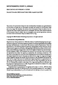
For any given initial surplus 𝑢 and insurer’s premium income per unit time 𝑐, the corresponding mean chance of the ultimate ruin could be calculated by MATLAB software. Figure 1 shows a plot of the mean chance of the ultimate ruin in the case of 𝑐 = 10. It sees that the mean chance of the ultimate ruin decreases from 0.64 to 7.2145 × 10−5 when 𝑢 increases from 0 to 500. Figure 2 shows a similar plot of the mean chance of the ultimate ruin under the conditions that 𝑐 = 20. Moreover, when 𝑢 increases from 0 to 500, the mean chance of the ultimate ruin decreases from 0.32 to 7.4351 × 10−14 . It shows from Figures 1 and 2 that their change features are similar as the initial surplus grows gradually. This accords with the practical running of insurance company and implies the significance of sufficient initial surplus. In addition, when insurer’s premium income per unit time 𝑐 equals 10 rather than 20, it is likely to occur earlier if the ultimate ruin appears. Example 2. Assume that the Poisson parameter 𝜆 = 0.6. Let an intuitionistic fuzzy random variable 𝜉̃1 = (𝜇𝜉̃ , ]𝜉̃ ) be given 1 1 by

14

Mathematical Problems in Engineering 0, { { { { { 𝑥 − 3𝜂 { { { { 𝜂 , 1 − ]𝜉̃ (𝑥) = { 1 { {1, { { { { { { 7𝜂 − 𝑥 , { 𝜂

0.7

Ch{T < ∞ | R(0) = u}

0.6 0.5 0.4

𝑥 < 3𝜂 or 𝑥 > 7𝜂, 3𝜂 ≤ 𝑥 < 4𝜂, (60)

4𝜂 ≤ 𝑥 < 6𝜂, 6𝜂 ≤ 𝑥 < 7𝜂.

For each given 𝜔 ∈ Ω and 𝛼 ∈ (0, 1], we have

0.3 0.2

𝑃 ̃𝜇 𝜉1,𝛼

(𝜔) = (3.5 + 0.5𝛼) 𝜂 (𝜔) ,

0.1

𝑂 ̃𝜇 𝜉1,𝛼

(𝜔) = (6.5 − 0.5𝛼) 𝜂 (𝜔) ,

𝑃 ̃1−] 𝜉1,𝛼

(𝜔) = (3 + 𝛼) 𝜂 (𝜔) ,

𝑂 ̃1−] 𝜉1,𝛼

(𝜔) = (7 − 𝛼) 𝜂 (𝜔) .

0

0

50

100 150 200 250 300 350 400 450 500 u

Figure 1: The mean chance of the ultimate ruin when 𝑐 = 10.

(61)

Ch{T < ∞ | R(0) = u}

Then 0.35

𝐸 [𝑃 𝜉̃1,𝛼 (𝜔)] = 𝐸 [(3.5 + 0.5𝛼) 𝜂 (𝜔)] = 3.5 + 0.5𝛼,

0.3

𝐸 [𝑂𝜉̃1,𝛼 (𝜔)] = 𝐸 [(6.5 − 0.5𝛼) 𝜂 (𝜔)] = 6.5 − 0.5𝛼,

𝜇 𝜇

0.25

1−] 𝐸 [𝑃 𝜉̃1,𝛼 (𝜔)] = 𝐸 [(3 + 𝛼) 𝜂 (𝜔)] = 3 + 𝛼,

0.2

1−] 𝐸 [𝑂𝜉̃1,𝛼 (𝜔)] = 𝐸 [(7 − 𝛼) 𝜂 (𝜔)] = 7 − 𝛼.

0.15

It follows that

0.1

Ch {𝑇 < ∞ | 𝑅 (0) = 𝑢} =

0.05 0

(62)

0

50

100 150 200 250 300 350 400 450 500 u

Figure 2: The mean chance of the ultimate ruin when 𝑐 = 20.

𝑥 − 3.5𝜂 { , { { 0.5𝜂 { { { { {1, 𝜇𝜉̃ (𝑥) = { 1 6.5𝜂 − 𝑥 { { { , { { { { 0.5𝜂 {0,

3.5𝜂 ≤ 𝑥 < 4𝜂,

⋅ ∫ (𝐸 [𝑃 𝜉̃1,𝛼 (𝜔)] ⋅ exp (− 𝜇

0

1−] + 𝐸 [𝑃 𝜉̃1,𝛼 (𝜔)] ⋅ exp (−

+ 𝐸 [𝑂𝜉̃1,𝛼 (𝜔)] ⋅ exp (− 𝜇

4𝜂 ≤ 𝑥 < 6𝜂, 6𝜂 ≤ 𝑥 < 6.5𝜂, (59)

where the random variable 𝜂 ∼ exp(1). Note that, for any given 𝜔 ∈ Ω, 𝜉̃1 (𝜔) is now assumed as a special trapezoidal intuitionistic fuzzy number. Then

=

𝑢

𝜇 𝐸 [𝑃 𝜉̃1,𝛼

(𝜔)]

𝑢

1−] 𝐸 [𝑃 𝜉̃1,𝛼 (𝜔)]

𝑢

𝜇 𝐸 [𝑂𝜉̃1,𝛼

1−] + 𝐸 [𝑂𝜉̃1,𝛼 (𝜔)] ⋅ exp (−

𝑥 ≤ 3.5𝜂 or 𝑥 ≥ 6.5𝜂,

1, 𝑥 < 3𝜂 or 𝑥 > 7𝜂, { { { { { 4𝜂 − 𝑥 { { { { 𝜂 , 3𝜂 ≤ 𝑥 < 4𝜂, ]𝜉̃ (𝑥) = { 1 { 0, 4𝜂 ≤ 𝑥 < 6𝜂, { { { { { { { 𝑥 − 6𝜂 , 6𝜂 ≤ 𝑥 < 7𝜂, { 𝜂

1

𝜆 𝜆 1 ⋅ exp ( 𝑢) ⋅ 𝑐 𝑐 4

(𝜔)]

1

0

+ (6.5 − 0.5𝛼) exp (−

)

(𝜔)]

3 3𝑢 1 ⋅ exp ( ) ⋅ 5𝑐 5𝑐 4

⋅ ∫ ((3.5 + 0.5𝛼) exp (−

)

𝑢

1−] 𝐸 [𝑂𝜉̃1,𝛼

𝑢 ) 3.5 + 0.5𝛼

𝑢 ) 6.5 − 0.5𝛼

+ (3 + 𝛼) exp (−

𝑢 ) 3+𝛼

+ (7 − 𝛼) exp (−

𝑢 )) 𝑑𝛼. 7−𝛼

)

)) 𝑑𝛼

(63)

Mathematical Problems in Engineering

15

Table 1: The mean chance values of the ultimate ruin. 2 0.5548 0.2613

3 0.5147 0.2283

4 0.4790 0.2001

5 0.4471 0.1759

6 0.4186 0.1550

7 0.3928 0.1370

8 0.3696 0.1214

0.7

0.35

0.6

0.3 Ch{T < ∞ | R(0) = u}

Ch{T < ∞ | R(0) = u}

𝑢 1 𝑐 = 5 0.6000 𝑐 = 10 0.3000

0.5 0.4 0.3 0.2 0.1 0

9 0.3485 0.1078

10 0.3293 0.0959

20 0.2033 0.0325

30 0.1364 0.0120

40 0.0944 0.0045

50 0.0662 0.0018

0.25 0.2 0.15 0.1 0.05

0

50

100 150 200 250 300 350 400 450 500 u

0

0

50

100 150 200 250 300 350 400 450 500 u

Figure 3: The mean chance of the ultimate ruin when 𝑐 = 5.

Figure 4: The mean chance of the ultimate ruin when 𝑐 = 10.

For any given initial surplus 𝑢 and insurer’s premium income per unit time 𝑐, the corresponding mean chance of the ultimate ruin could be calculated by MATLAB software. Figure 3 shows a plot of the mean chance of the ultimate ruin in the case of 𝑐 = 5, in which the mean chance of the ultimate ruin decreases from 0.6 to 2.1642 × 10−7 when 𝑢 increases from 0 to 500. Figure 4 shows a similar plot of the mean chance of the ultimate ruin under the conditions that 𝑐 = 10. Moreover, the mean chance of the ultimate ruin decreases from 0.3 to 1.0126 × 10−20 when 𝑢 increases from 0 to 500. Table 1 presents the corresponding results of the mean chance of the ultimate ruin as 𝑢 increases from 1 to 50 in the cases of 𝑐 = 5 and 𝑐 = 10, respectively. This shows that their features agree with the practical running of insurance company.

in uncertain decision systems based on intuitionistic fuzzy random variables. And the research of uncertain random programming by effectively integrating uncertain theory and probability theory will be discussed in the near future.

7. Conclusion

References

This paper proposes a novel definition of intuitionistic fuzzy random variable, establishes a scalar expectation value of intuitionistic fuzzy random variable, and discusses their measurability properties. Considering the individual claim amount in insurance company as an intuitionistic fuzzy random variable, a risk model, where the claim number process is considered to be a Poisson process, has been given. Moreover, when the individual claim amount is characterized as an exponentially distributed intuitionistic fuzzy random variable, the expressions for the mean chance of the ultimate ruin are obtained with initial surplus or without initial surplus, respectively. Last but not least, two illustrated examples are given to show the feasibility of the approach. Intuitionistic fuzzy random variables are effective mathematical tools for dealing with high-uncertainty phenomena. A further issue worthy of consideration will be the application

[1] M. Lo´eve, Probability Theory, Van Nostrand Co., Inc., Princeton, NJ, USA, 3rd edition, 1963. [2] D. Dubois and H. Prade, Possibility Theory, Plenum Press, New York, NY, USA, 1988. [3] L. A. Zadeh, “The concept of a linguistic variable and its application to approximate reasoning-III,” Information Sciences, vol. 9, no. 1, pp. 43–80, 1975. [4] L. A. Zadeh, “Fuzzy sets as a basis for a theory of possibility,” Fuzzy Sets and Systems, vol. 1, no. 1, pp. 3–28, 1978. [5] H. Kwakernaak, “Fuzzy random variables. I. Definitions and theorems,” Information Sciences, vol. 15, no. 1, pp. 1–29, 1978. [6] M. L. Puri and D. A. Ralescu, “Fuzzy random variables,” Journal of Mathematical Analysis and Applications, vol. 114, no. 2, pp. 409–422, 1986. [7] Y. K. Liu and B. Liu, “Expected value operator of random fuzzy variable and random fuzzy expected value models,”

Conflicts of Interest The authors declare that there are no conflicts of interest regarding the publication of this paper.

Acknowledgments This work is supported by the National Natural Science Foundation of China (Grants nos. 11401495 and 11401494).

16

[8]

[9]

[10]

[11]

[12]

[13]

[14]

[15]

[16]

[17]

[18]

[19]

[20]

[21] [22] [23] [24]

[25]

[26]

Mathematical Problems in Engineering International Journal of Uncertainty, Fuzziness and KnowledgeBased Systems, vol. 11, no. 2, pp. 195–215, 2003. R. Kruse and K. D. Meyer, Statistics with vague data, Theory and Decision Library. Series B: Mathematical and Statistical Methods, D. Reidel Publishing Co., Dordrecht, Holland, 1987. Y. K. Liu and B. Liu, “Fuzzy random variables: a scalar expected value operator,” Fuzzy Optimization and Decision Making. A Journal of Modeling and Computation Under Uncertainty, vol. 2, no. 2, pp. 143–160, 2003. C. V. Negoita and D. Ralescu, Simulation, Knowledge-based Computing and Fuzzy Statistics, Van Nostrand Reinhold Company, New York, NY, USA, 1987. M. L. Puri and D. A. Ralescu, “The concept of normality for fuzzy random variables,” Annals of Probability, vol. 13, no. 4, pp. 1373–1379, 1985. X. Bai, “Two-stage multiobjective optimization for emergency supplies allocation problem under integrated uncertainty,” Mathematical Problems in Engineering, Article ID 2823835, 13 pages, 2016. R. Gao and K. Yao, “Importance index of components in uncertain random systems,” Knowledge-Based Systems, vol. 109, pp. 208–217, 2016. Y. Liu, Z. Qiao, and G. Wang, “Fuzzy random reliability of structures based on fuzzy random variables,” Fuzzy Sets and Systems, vol. 86, no. 3, pp. 345–355, 1997. M. Zhang, S. Lu, and B. Li, “A fuzzy reliability model of blades to avoid resonance and its convergence analysis,” Mathematical Problems in Engineering, vol. 2014, Article ID 278342, 2014. Y. Liu, “Uncertain random programming with applications,” Fuzzy Optimization and Decision Making. A Journal of Modeling and Computation Under Uncertainty, vol. 12, no. 2, pp. 153–169, 2013. Y. Liu and D. A. Ralescu, “Risk index in uncertain random risk analysis,” International Journal of Uncertainty, Fuzziness and Knowledge-Based Systems, vol. 22, no. 4, pp. 491–504, 2014. Y. K. Liu and B. Liu, “On minimum-risk problems in fuzzy random decision systems,” Computers & Operations Research, vol. 32, no. 2, pp. 257–283, 2005. T. Huang, R. Zhao, and W. Tang, “Risk model with fuzzy random individual claim amount,” European Journal of Operational Research, vol. 192, no. 3, pp. 879–890, 2009. Q. Shen and R. Zhao, “Risk assessment of serious crime with fuzzy random theory,” Information Sciences, vol. 180, no. 22, pp. 4401–4411, 2010. B. Liu, “Why is there a need for uncertainty theory?” Journal of Uncertain Systems, vol. 6, no. 1, pp. 3–10, 2012. B. Liu, Uncertainty Theory, Springer, Berlin, Germany, 2004. S. Wang and J. Watada, Fuzzy stochastic optimization, Springer, New York, 2012. S. M. Wang, Y. K. Liu, and J. Watada, “Fuzzy random renewal process with queueing applications, Computers Mathematics with Applications,” Elsevier Publisher, vol. 57, no. 7, pp. 1232– 1248, 2009. S. Wang and J. Watada, “Fuzzy random renewal reward process and its applications,” Information Sciences, vol. 179, no. 23, pp. 4057–4069, 2009. S. Wang and W. Pedrycz, “Robust granular optimization: a structured approach for optimization under integrated uncertainty,” IEEE Transactions on Fuzzy Systems, vol. 23, no. 5, pp. 1372–1386, 2015.

[27] S. Wang, B. Wang, and J. Watada, “Adaptive Budget-Portfolio Investment Optimization Under Risk Tolerance Ambiguity,” IEEE Transactions on Fuzzy Systems, vol. 25, no. 2, pp. 363–376, 2017. [28] K. T. Atanassov, “Intuitionistic fuzzy sets,” Fuzzy Sets and Systems, vol. 20, no. 1, pp. 87–96, 1986. [29] T.-Y. Chen, “IVIF-PROMETHEE outranking methods for multiple criteria decision analysis based on interval-valued intuitionistic fuzzy sets,” Fuzzy Optimization and Decision Making, vol. 14, no. 2, pp. 173–198, 2015. [30] B. Liu, Y. Shen, W. Zhang, X. Chen, and X. Wang, “An interval-valued intuitionistic fuzzy principal component analysis model-based method for complex multi-attribute largegroup decision-making,” European Journal of Operational Research, vol. 245, no. 1, pp. 209–225, 2015. [31] P. Liu and F. Jin, “Methods for aggregating intuitionistic uncertain linguistic variables and their application to group decision making,” Information Sciences, vol. 205, pp. 58–71, 2012. [32] Z. S. Xu and J. Chen, “An overview of distance and similarity measures of intuitionistic fuzzy sets,” International Journal of Uncertainty, Fuzziness and Knowledge-Based Systems, vol. 16, no. 4, pp. 529–555, 2008. [33] Z. Pei, “Intuitionistic fuzzy variables: concepts and applications in decision making,” Expert Systems with Applications, vol. 42, no. 22, pp. 9033–9045, 2015. [34] Z. Zainali, M. G. Akbari, and H. Alizadeh Noughabi, “Intuitionistic fuzzy random variable and testing hypothesis about its variance,” Soft Computing, vol. 19, no. 9, pp. 2681–2689, 2015. [35] B. Liu and Y. K. Liu, “Expected value of fuzzy variable and fuzzy expected value models,” IEEE Transactions on Fuzzy Systems, vol. 10, no. 4, pp. 445–450, 2002. [36] H. U. Gerber, An Introduction to Mathematical Risk Theory, vol. 8 of S.S. Heubner Foundation Monograph Series, University of Pennsylvania, Philadelphia, Pa, USA, 1979.

Advances in

Operations Research Hindawi www.hindawi.com

Volume 2018

Advances in

Decision Sciences Hindawi www.hindawi.com

Volume 2018

Journal of

Applied Mathematics Hindawi www.hindawi.com

Volume 2018

The Scientific World Journal Hindawi Publishing Corporation http://www.hindawi.com www.hindawi.com

Volume 2018 2013

Journal of

Probability and Statistics Hindawi www.hindawi.com

Volume 2018

International Journal of Mathematics and Mathematical Sciences

Journal of

Optimization Hindawi www.hindawi.com

Hindawi www.hindawi.com

Volume 2018

Volume 2018

Submit your manuscripts at www.hindawi.com International Journal of

Engineering Mathematics Hindawi www.hindawi.com

International Journal of

Analysis

Journal of

Complex Analysis Hindawi www.hindawi.com

Volume 2018

International Journal of

Stochastic Analysis Hindawi www.hindawi.com

Hindawi www.hindawi.com

Volume 2018

Volume 2018

Advances in

Numerical Analysis Hindawi www.hindawi.com

Volume 2018

Journal of

Hindawi www.hindawi.com

Volume 2018

Journal of

Mathematics Hindawi www.hindawi.com

Mathematical Problems in Engineering

Function Spaces Volume 2018

Hindawi www.hindawi.com

Volume 2018

International Journal of

Differential Equations Hindawi www.hindawi.com

Volume 2018

Abstract and Applied Analysis Hindawi www.hindawi.com

Volume 2018

Discrete Dynamics in Nature and Society Hindawi www.hindawi.com

Volume 2018

Advances in

Mathematical Physics Volume 2018

Hindawi www.hindawi.com

Volume 2018