Hindawi Publishing Corporation International Journal of Distributed Sensor Networks Volume 2014, Article ID 218678, 13 pages http://dx.doi.org/10.1155/2014/218678
Research Article A Scheduled Activity Energy Aware Distributed Clustering Algorithm for Wireless Sensor Networks with Nonuniform Node Distribution Nooshin Nokhanji, Zurina Mohd Hanapi, Shamala Subramaniam, and Mohamad Afendee Mohamed Department of Communication Technology and Network, Faculty of Computer Science and Information Technology, Universiti Putra Malaysia, 43400 Serdang, Selangor, Malaysia Correspondence should be addressed to Nooshin Nokhanji; nooshin
[email protected] Received 13 February 2014; Revised 12 May 2014; Accepted 20 May 2014; Published 3 July 2014 Academic Editor: Jiun-Long Huang Copyright © 2014 Nooshin Nokhanji et al. This is an open access article distributed under the Creative Commons Attribution License, which permits unrestricted use, distribution, and reproduction in any medium, provided the original work is properly cited. Nonuniform node deployment makes the cluster-based routing protocol less efficient in wireless sensor networks (WSNs). Energy aware distributed clustering (EADC) is one of the cluster-based routing protocols proposed for networks with nonuniform node distribution, which can effectively balance the energy consumption among the nodes. However, due to the nonuniform node distribution, there is a redundancy in sensed and transmitted data in dense area. This unnecessary energy consumption is not considered in EADC. Therefore, in this paper, a new algorithm called scheduled activity EADC (SA-EADC) is proposed. SAEADC exploits the redundant nodes and turns them off for the current round. The redundant nodes are scheduled based on their residual energy to work alternatively. The results show that SA-EADC significantly decreases the energy consumption and extends the network lifetime without degradation in coverage and sensing reliability of the network.
1. Introduction Wireless sensor networks (WSNs) consist of a hundred to a thousand sensor nodes, which measure a property from the environment as well as processing and transmitting the collected data to the base station (BS) [1]. However, they have many constraints, because the sensor nodes have limited capabilities. Since the energy resources of the sensor nodes are limited and nonrechargeable, energy efficiency is a very critical issue in the design of the network topology, which affects the network lifetime significantly. Hence, the main concern in designing protocols is how to reduce the energy consumption and extend the network lifetime [2]. It has been proved by many researchers that among different categories of routing protocols based on the network architecture, cluster-based (hierarchical) routing protocols are more energy efficient and increase the scalability as well as lifetime of the network [3–5]. Clustering schemes divide the field into multiple clusters, where each cluster is controlled by a cluster head (CH) with the purpose of gathering data
from cluster members (CM). CHs act as the local BS for their own clusters. After gathering data and performing data aggregation to omit the redundant data, the data are transmitted to the BS [6–8]. Networks with nonuniform node distribution make the cluster-based routing protocols less efficient [9, 10]. The nonuniform node deployment makes the energy consumption of the nodes more imbalanced [9]. Furthermore, as the density of the sensor nodes varies in each region due to nonuniform node distribution, in dense area the sensed and transmitted data are extremely correlated and redundant. In random and nonuniform node distribution, there may exist some redundant sensor nodes whose coverage areas are completely covered by their neighbor nodes. These redundant sensor nodes can be identified and scheduled to be activated alternatively in order to prolong the network lifetime [11]. Energy aware distributed clustering (EADC) [9] is one of the protocols proposed for networks with nonuniform node distribution, which can effectively balance the energy consumption among the nodes. However, the unnecessary
2 energy consumption of redundant nodes is not considered in EADC. Therefore, in this paper, a scheduled activity energy aware distributed clustering (SA-EADC) is proposed based on EADC, which exploits the redundant nodes and turns them off. The redundant nodes are scheduled based on their residual energy to work alternatively. The proposed algorithm maintains the original sensing coverage and guarantees a certain redundancy. Consequently, SA-EADC avoids unnecessary redundant sensing and transmission of data, which reduces the overall energy consumption and extends the lifetime of the network. The rest of the paper is organized as follows. Section 2 covers the related works in this area. Section 3 introduces the network model of our algorithm. Section 4 explains the used redundancy check method and activity-scheduling algorithm in SA-EADC. Section 5 presents SA-EADC in detail. Section 6 analyzes the properties of the proposed protocol. Section 7 describes the simulation and the analysis of the obtained results. Finally, the paper is concluded in Section 8.
2. Related Work In this section, first some typical energy efficient clustering protocols are discussed. Afterwards, the sensor node scheduling algorithms are analyzed, which focuses on exploiting the redundant nodes and scheduling their activity. 2.1. Energy Efficient Clustering Protocols. Low energy adaptive clustering hierarchy (LEACH) [5] is a fundamental clustering algorithm, in which the sensor nodes independently elect themselves as the CH. The CHs are responsible to gather the data from their CMs, perform data aggregation to omit the redundant data, and transmit data to the BS using single hop communication. The nodes are selected as the CHs in turn with the purpose of evenly distributing energy expenditure in the network. Despite of being simple, the remaining energy of nodes is not considered as a parameter in CH selection. Moreover, it is not suitable for the large size networks. Thus, several cluster-based routing protocols were proposed so as to tackle the limitations of LEACH and improve its performance [13–15]. Energy efficient heterogeneous clustered (EEHC) routing protocol proposed by Kumar et al. [16] considers a network with the nodes, which differ in their energy level. CH selection and cluster formation are performed in a distributed method. The CH selection phase is performed based on the residual energy of the nodes. Nevertheless, the intercluster communication phase is performed in single hop and the residual energy of the nodes is not considered in CH selection. Energy-aware data gathering (EADEEG) [17] is another clustering routing protocol, which is able to achieve a good CH distribution. The CHs are selected according to the residual energy of the nodes and the average residual energy of their neighbors in EADEEG. In spite of improving the network lifetime, EADEGG suffers from the existence of “isolated points” [4]. Yu et al. [4] proposed energy aware distributed unequal clustering (EADUC) routing protocol in order to solve
International Journal of Distributed Sensor Networks the mentioned problem in EADEGG. EADUC assumes a network with heterogeneous nodes, which are different in energy resources. Additionally, the clusters are constructed in unequal sizes in EADUC, in order to solve the “hotspot” problem. The hot spot problem is related to the early death of CH nodes, which are closed to the BS. Therefore, the clusters near to the BS have smaller size to save more energy for intercluster communication. Arranging cluster sizes and transmission ranges (ACT) proposed by Lai et al. [7] is a novel clustering routing protocol. ACT separates the network topology into multiple levels. The sizes of the clusters are the same in each level and are different from other levels. In other words, the clusters near to the BS are the smallest, whereas the largest clusters are the farthest ones from the BS to overcome the problem of “hot spot.” Since ACT avoids reclustering in each round, a cluster maintenance phase was proposed. Cluster maintenance phase consists of CH rotation based on energy threshold and crosslevel data transmission. The results show that ACT can significantly increase the network lifetime. However, it does not address the coverage problem [7]. In addition, although cluster sizes are arranged according to energy consumption, the location of the newly selected CH strays from the ideal ones. This issue makes the distribution of energy fluctuate [18]. Coverage preservation clustering protocol (CPCP) [19] is a clustering protocol in which the clusters are constructed based on a group of coverage-aware metrics [2]. It considers a network with nonuniform node distribution. The main concern of CPCP is coverage preservation and it uses good CH selection technique. However, the network lifetime and balancing energy expenditure are not noted in detail in CPCP [9]. 2.2. Sensor Activity Scheduling Protocols. In [20], Cardei and Du proposed a method in order to preserve full coverage of the area, in which the sensor nodes are divided into disjoint cover sets. These cover sets are active alternatively. Each cover set contains adequate number of active sensor nodes, which are essential to cover the monitoring area, meanwhile the rest of the sensor nodes are turned off. While, the rest of the sensor nodes are turned off. However, this scheme is based on a centralized approach. Therefore, it requires global synchronization overhead; besides it is not scalable in the networks with large size. In PEAS [21], the sensor nodes use a simple rule in order to decide about their activity. The sensor node will be active if it cannot find another active node in its probing range. Otherwise, it will return to the sleep mode. PEAS does not require the nodes to maintain the neighbor state and location information. Therefore, it reduces the complexity. However, it does not guarantee a complete coverage preservation of the environment [22]. Tian and Georganas in [22] proposed a scheduling scheme, in which the sensor nodes decide about their state in a distributed manner, based on the obtained coverage information from their neighbors. In this scheme, in order to avoid creation of “blind points” in the network, a random back-off time is introduced, before a node makes a decision
International Journal of Distributed Sensor Networks
3
about its status. The problem of “blind points” occurs when two sensor nodes, whose redundancy is dependent to each other, decide to be inactive simultaneously. In CPCP clustering scheme [19], in order to check the redundancy, the grid approach is used. Although this method is a straightforward approach and it does not limit the sensing coverage model, it can be time consuming, storage expensive, and computation complicated [12]. Soro and Heinzelman introduced a delay in node activation based on the nodes current cost value in order to avoid “blind point” problem. Therefore, the nodes with less cost have a better chance to be inactive. In BCA clustering scheme [10], in order to identify inactive nodes, each CH calculates the average number of nodes in a cluster. The number of inactive sensor nodes is equal to the difference of the nodes in a cluster from the average number of nodes. The CHs select the inactive nodes randomly and each selected sensor node determines whether to be inactive or not. Although it is a simple method, the full coverage is not guaranteed in this approach.
3. Network Model There are 𝑁sensor nodes distributed in 𝑀 × 𝑀 square field in the network. Each node has a unique identity. The BS and the sensor nodes are stationary after deployment. Nodes are heterogeneous in terms of energy and location unawareness. All sensor nodes can use power control to vary the amount of transmit power. The BS is out of the field. It has sufficient energy resource and the location of the BS is known by each node. The communication link is symmetrical. The sensor nodes are able to estimate the distance between sender and receiver by the received signal strength indication. The sensor nodes are time synchronized and their failure is due to the energy depletion. The energy model used in SA-EADC is adopted from LEACH [5]. In order to transmit 𝑙 bit message to the distance of 𝑑, the energy dissipates as follows: 𝑙 × 𝐸elec + 𝑙 × ∈𝑓𝑠 × 𝑑2 , 𝐸𝑇𝑋 (𝑙, 𝑑) = { 𝑙 × 𝐸elec + 𝑙 × ∈𝑚𝑝 × 𝑑4 ,
𝑑 ≤ 𝑑0 𝑑 ≥ 𝑑0 ,
(1)
where 𝐸elec is the energy dissipation to run the radio electronics and ∈𝑓𝑠 and ∈𝑚𝑝 are the energy dissipation values to run the amplifier for close and far distances, respectively. For receiving 𝑙 bit message, the radio dissipates energy as follows: 𝐸𝑅𝑋 (𝑙) = 𝑙 × 𝐸elec .
(2)
In addition, it is assumed that the energy consumptions due to data sensing and data aggregation are 𝐸sen and 𝐸com , respectively.
4. Sensor Activity Scheduling In order to schedule the sensor activity to preserve the complete coverage of area, the first question is to find out whether the area covered by the sensor node is covered completely by its active neighbors. It should be noted that
Rs
S4 P1 S1
S3
Rs
P3 P2
S2
Rs
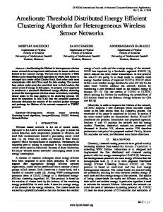
Figure 1: Crossing coverage redundancy check method [12].
the state of the nodes’ neighbor has a significant impact on the redundancy of the node. A node may not be redundant anymore, if one of its active neighbors becomes inactive. The second question is to identify the order of sensor’s activation and deactivation [12]. The following sections describe the redundancy check method and activity scheduling procedure used in SA-EADC. 4.1. Redundancy Check Method. SA EADC utilizes the crossing coverage redundancy check method proposed by Xing et al. [23] in order to determine the redundant nodes, since it reduces the storage requirements and computation complexity [12]. If the sensing disks of two nodes intersect each other, then crossing points that are the intersection points on the perimeters of two disks will be created. As represented in Figure 1, 𝑆2 and 𝑆3 disk perimeters created crossing point 𝑃1 inside the sensing disk 𝑆1 . The point on the sensing disk perimeter of a sensor is not considered as covered by the sensor itself. Thus, sensors 𝑆1 and 𝑆2 do not cover crossing point 𝑃1 , whereas, 𝑃1 is covered by 𝑆4 . Consequently, 𝑃1 is a covered crossing inside sensing disk of sensor 𝑆1 . The redundancy rule of crossing coverage is explained as follows: “If all the crossings within the sensor’s sensing disk are covered, then sensor 𝑆 will be redundant and eligible to be inactive.” As it is shown in Figure 1, since all the crossing points inside sensing disk of 𝑆1 are covered, it is a redundant node and it can go into sleep mode. 4.2. Activity Scheduling Procedure. A fully distributed “selfinactivation” algorithm is proposed in order to determine the order of sensor’s activation and deactivation and avoid creation of “blind points,” since the centralized algorithms are not scalable and need global synchronization overhead. The proposed algorithm avoids the problem of “blind points” by introducing the delay in the node deactivation based on the residual energy of the node. Therefore, the sensor nodes with higher remaining energy have a higher chance to be active in each round. The activity scheduling procedure of SA-EADC is discussed in detail in following section.
4
International Journal of Distributed Sensor Networks
begin (information collection algorithm) 𝑠𝑡𝑎𝑡𝑒 ← 𝐶𝑎𝑛𝑑𝑖𝑑𝑎𝑡𝑒 𝑠𝑡𝑎𝑡𝑢𝑠 ← 𝐴𝑐𝑡𝑖V𝑒 while (𝑇1 has not expired) do Receive 𝑁𝑜𝑑𝑒 𝑀𝑠𝑔 Update neighborhood table NT [ ] Update active direct neighbor table ADNT [ ] end 𝑡𝑖 ← broadcast delay time for competing a cluster head end Pseudocode 1: Pseudocode of information collection phase in SA-EADC.
Table 1: Description of control messages in SA-EADC. Control messages Node Msg
Description Tuple (selfid, selfenergy)
Head Msg
Tuple (selfid)
Join Msg
Tuple (selfid, headed)
Schedule Msg
Tuple (schedule order)
Sleep Msg
Tupple (selfid, slefstatus)
Route Msg
Tuple (selfid, selfenergy, membernum, disttoBS)
5. SA-EADC Algorithm In this section, SA-EADC clustering algorithm is introduced in detail. Similar to EADC, the protocol contains an energy aware clustering algorithm (SA-EADC) and a cluster-based routing algorithm. SA-EADC adds a “sensor redundancy check and activation” phase to EADC. Thus, it makes even clusters. Furthermore, a subset of sensor nodes is selected to perform the sensing task while the redundant sensor nodes go to sleep mode for the current round. SA-EADC not only maintains the original coverage area, but also maintains a certain redundancy to guarantee the sensing reliability of the system. In the cluster-based routing algorithm, which is identical to [9], the energy consumption among the CHs is balanced. The description of the control messages used in the process of SA-EADC is shown in Table 1. 5.1. SA-EADC Details. The clustering process of SA-EADC is divided into four phases: information collection phase with duration of 𝑇1 , cluster head competition phase with the duration of 𝑇2 , sensor redundancy check and activation phase with duration of 𝑇3 , and cluster formation phase with duration of 𝑇4 . 5.1.1. Information Collection Phase. The duration of this phase is defined as 𝑇1 , in which the status of all the nodes is set to “Active.” Identical to “information collection phase” in EADC, each node broadcasts a “Node Msg.” This message consists of two values: the node ID and residual energy of the node within the radio range 𝑟. At the same time, each node receives “Node Msg” messages from its neighbors. Afterwards, the sensor nodes start identifying their list of neighbors and build the list of active direct neighbors based
on the received “Node msg.” Two sensor nodes are called direct neighbor if 𝑑(𝑆1 , 𝑆2 ) < 2𝑅𝑠 , where 𝑅𝑠 is the sensing range of the sensor node. Then each node starts to calculate the average residual energy of its neighbors 𝐸𝑖𝑎 using 𝐸𝑖𝑎 =
1 𝑑 ∑𝐸 , 𝑑 𝑗=1 𝑗𝑟
(3)
where 𝐸𝑗𝑟 is the residual energy of 𝑆𝑗 (one neighbor node of 𝑆𝑖 ) and 𝑑 is the number of the neighbors of 𝑆𝑖 . Afterwards, each node uses (4) in order to calculate its waiting time for broadcasting “Head Msg”: 𝐸 { 𝑖𝑎 𝑇2 𝑉𝑟 , 𝐸𝑖𝑟 ≥ 𝐸𝑖𝑎 (4) 𝑡𝑖 = { 𝐸𝑖𝑟 𝑇 𝑉 𝐸 < 𝐸 , 𝑖𝑟 𝑖𝑎 { 2 𝑟 where 𝑡𝑖 and 𝐸𝑖𝑟 are waiting time and residual energy of 𝑆𝑖 , respectively, and 𝑉𝑟 is a real value uniformly distributed in [0.9, 1]. This value is introduced to reduce the probability that two nodes simultaneously send the “Head Msg.” The pseudocode of this phase is shown in Pseudocode 1. 5.1.2. Cluster Head Competition Phase. Afterwards, SAEADC starts the CH competition phase, whose duration is 𝑇2 . In this phase, if the sensor node does not receive any “Head Msg” during the expiration of timer 𝑡𝑖 , it will broadcast the “Head Msg” in order to advertise itself as a CH within the radio range 𝑅𝐶. Otherwise, the sensor node gives up the competition. Pseudocode 2 shows the pseudocode of this phase. 5.1.3. Sensor Redundancy Check and Activation Phase. As 𝑇2 expires, SA-EADC begins the sensor redundancy check and activation phase whose duration is 𝑇3 . During this phase, the plain nodes check their redundancy and their activity is scheduled. Note that the selected CH sensor nodes should be active in each round. Since all the sensor nodes know their state (i.e., plain or CH), all the non-CH nodes jointly participate in this phase without considering to which cluster they belong. This scheme prevents the redundant activation of sensors on the boundary of clusters, which may occur when the activation of nodes is performed independently in each cluster. Each plain node performs “crossing coverage”
International Journal of Distributed Sensor Networks
5
begin (cluster head competition algorithm) while (𝑇2 has not expired) do if 𝐶𝑢𝑟𝑟𝑒𝑛𝑡𝑇𝑖𝑚𝑒 < 𝑡𝑖 do if receive a 𝐻𝑒𝑎𝑑 𝑀𝑠𝑔 from a neighbor NT [𝑗] do 𝑠𝑡𝑎𝑡𝑒 ← 𝑃𝑙𝑎𝑖𝑛 NT [𝑗] ⋅ 𝑠𝑡𝑎𝑡𝑒 ← 𝐻𝑒𝑎𝑑 else Continue end else if 𝑠𝑎𝑡𝑒 = 𝐶𝑎𝑛𝑑𝑖𝑑𝑎𝑡𝑒 do 𝑠𝑡𝑎𝑡𝑒 ← 𝐻𝑒𝑎𝑑 Broadcast 𝐻𝑒𝑎𝑑 𝑀𝑠𝑔 end end end Pseudocode 2: Pseudocode of cluster head competition phase.
begin (sensor redundancy check and activation algorithm) while (𝑇3 has not expired) do if 𝑠𝑡𝑎𝑡𝑒 = 𝑃𝑙𝑎𝑖𝑛 and location ≠ on boundary do Execute the crossing coverage algorithm while (𝐼𝑠𝑅𝑒𝑑𝑢𝑛𝑑𝑎𝑛𝑡 = 𝑇𝑟𝑢𝑒) do Set Timer 𝛼 𝐸residual Wait for Timer expiration if receive a 𝑆𝑙𝑒𝑒𝑝 𝑀𝑠𝑔 from an active direct neighbor do Update active direct neighbor table ADNT [ ] Execute the crossing coverage algorithm else Broadcast 𝑆𝑙𝑒𝑒𝑝 𝑀𝑠𝑔 𝑆𝑡𝑎𝑡𝑢𝑠 ← 𝐼𝑛𝑎𝑐𝑡𝑖V𝑒 end end end end end Pseudocode 3: Pseudocode of sensor redundancy check and activity scheduling phase.
redundancy check method [23] to identify whether its complete coverage area is preserved or not. However, the edge nodes (i.e., the nodes that are placed at the boundary of the field) have no chance to be inactive, since all other nodes are located at one side of the edge nodes [22]. If the sensor node determines itself as the redundant, it will set a timer proportional to its residual energy level. Otherwise, its status will be remained as active for the current round. Note that when a redundant sensor node has higher residual energy level, its timer will last longer. Therefore, this sensor node has a higher priority to be active during the current round. Furthermore, setting the timer proportional to the energy level avoids creation of coverage holes. Furthermore, setting the timer proportional to the energy level avoids creation of coverage holes, because none of the redundant nodes will not go to sleep mode at the same time. Afterwards, the redundant nodes wait for timer expiration. If the sensor node receives no “Sleep Msg” during its timer expiration, it will set its status to inactive, broadcast a “Sleep Msg” in range of 2𝑅𝑠 , which
includes the ID of the node and its status, and go to sleep mode for the current round. Otherwise, it will rebuild the list of its active direct neighbors and perform the redundancy check method again to determine whether it is redundant anymore or not. The pseudocode of this phase is shown in Pseudocode 3. 5.1.4. Cluster Formation Phase. In this phase, all the active plain nodes select a CH, according to the received signal strength. Thus, they will select the nearest CH and send the “Join Msg.” The CHs create a node-scheduling list based on the received “Join Msg.” CHs create and send the “schedule Msg” in order to identify the time of data transmission for the nodes and, in other times, they can be in the sleep mode. This issue will result in saving energy. Pseudocode 4 shows the pseudocode of cluster formation phase. At this point, the whole process of SA-EADC is done. The clusters consist of the nodes in Voronoi cell around the CHs.
6
International Journal of Distributed Sensor Networks
begin (cluster formation algorithm) while (𝑇4 has not expired) do if 𝑠𝑡𝑎𝑡𝑒 = 𝑃𝑙𝑎𝑖𝑛 && 𝑠𝑡𝑎𝑡𝑢𝑠 = 𝐴𝑐𝑡𝑖V𝑒 && has not sent 𝐽𝑜𝑖𝑛 𝑀𝑠𝑔 do Send 𝐽𝑜𝑖𝑛 𝑀𝑠𝑔 to the nearest cluster head else if 𝑠𝑡𝑎𝑡𝑒 = 𝐻𝑒𝑎𝑑 do Receive 𝐽𝑜𝑖𝑛 𝑀𝑠𝑔 from its 𝐴𝑐𝑡𝑖V𝑒 neighbor 𝑃𝑙𝑎𝑖𝑛 nodes end end if 𝑠𝑡𝑎𝑡𝑒 = 𝐻𝑒𝑎𝑑 do Broadcast 𝑆𝑐ℎ𝑒𝑑𝑢𝑙𝑒 𝑀𝑠𝑔 end end Pseudocode 4: Pseudocode of cluster formation phase protocol analysis.
5.2. Cluster-Based Routing Algorithm. SA-EADC utilizes the cluster-based routing algorithm of EADC [9]. Similar to EADC, the CHs generated by EADC distribute uniformly over the network. Therefore, the size of clusters is equal. However, due to the nonuniform node distribution, clusters in the dense area have more members in comparison to the clusters in the sparse area. Hence, this issue results in imbalanced energy consumption of CHs. According to Yu et al. [9] the energy consumption in multihop communication is divided into intracluster energy consumption and intercluster energy consumption. The CHs consume energy due to receiving, aggregating and transmitting data from their CMs, which is called intracluster energy consumption. In addition, they consume energy due to forwarding data for their neighbor CHs, which is called intercluster energy consumption. Yu et al. [9] adjusted the ratio of two parts of energy consumption, in order to balance the energy consumption among the CHs. The CHs in sparse area forward more data packet to mitigate the imbalance intracluster energy consumption. Furthermore, the heterogeneity of the nodes is also taken into consideration. Thus, if the CHs with higher residual energy are chosen to take more forwarding task, the network lifetime will be better prolonged. At the beginning of this phase, each CH broadcasts a “Route MSG” message within the radius range 𝑅𝑟 . This control message contains the values of remaining energy, the number of CMs, and the distance to the BS itself. If the distance of the CH to BS is less than an identified threshold, it will set the BS as its next hop. Otherwise, according to the received “Route MSG,” it will choose a CH as the next hop with higher residual energy, smaller number of members, and no further away from BS. The value of “relay” is calculated using the following formula, when CH 𝑆𝑖 chooses CH 𝑆𝑗 as its next hop: 𝐸𝑗𝑟 1 + (1 − 𝛼) , relay (𝑆𝑖 , 𝑆𝑗 ) = 𝛼 (5) 𝐸max 𝑆𝑗(cm−num) where 𝐸𝑗𝑟 is the residual energy of the CH 𝑆𝑗 , 𝐸max is the maximum initial energy of nodes in the network. 𝑆𝑗(cm−num) is the number of CMs of 𝑆𝑗 , and 𝛼 is a real value uniformly distributed in [0, 1]. It determines which factor is more important in selection of next hop. It is obvious from the
equation that a CH with higher remaining energy and fewer CMs will have a larger value of “relay.” A neighbor CH with a highest “relay” and closer to the BS will be selected as the next hop. If there is more than one CH with equal and largest relay value, the one, which has a farther distance to the BS, will be chosen. The reason is to prevent premature death of the CHs near the BS because of forwarding much load. The pseudocode of this phase is shown in Pseudocode 5. 5.3. Data Transmission Phase. Data transmission phase is composed of intracluster communication and intercluster communication phase. These phases are discussed as follows. 5.3.1. Intracluster Communication Phase. CMs collect the data from the monitoring area and transmit the data in the allocated time slot to their CH directly. 5.3.2. Intercluster Communication Phase. CHs receive data from their members, perform data aggregation, and send the aggregated data to the next hop nodes. If a CH receives the data from other CHs, it will forward it to the next hop, without performing data aggregation. The topology of SA-EADC is shown in Figure 2.
6. Protocol Analysis Theorem 1. The overhead complexity of control messages in the network is 𝑂(𝑁). Proof. In each clustering process, each node broadcasts a Node Msg. Therefore, there are 𝑁 Node Msg. In each round, each active sensor node broadcasts a Join Msg. Each CH broadcasts a Head Msg, a Schedule Msg, and a Route Msg, while, each inactive node broadcasts a Sleep Msg. Suppose the number of inactive sensor nodes and the number of generated CH are 𝑆 and 𝐾, respectively. Therefore, the total number of control message in the whole network is 𝑁 + (𝑁 − 𝐾 − 𝑆) + 𝐾 + 𝐾 + 𝐾 + 𝑆 = 2𝑁 + 2𝐾, which is a linear function of 𝑁. Therefore, the overhead complexity of control messages in the network is 𝑂(𝑁). Theorem 2. SA-EADC can set up the clustering topology in 𝑂(1) time.
International Journal of Distributed Sensor Networks
7
Rc
BS
DIST TH
Cluster head node Active node Inactive node
Figure 2: Topology of SA-EADC.
begin (cluster-based routing algorithm) Broadcast 𝑅𝑜𝑢𝑡𝑒 𝑀𝑠𝑔 if 𝑑𝑖𝑠𝑡𝑡𝑜𝐵𝑆 < 𝐷𝐼𝑆𝑇 𝑇𝐻 do 𝑛𝑒𝑥𝑡ℎ𝑜𝑝 ← 𝐵𝑆 else while (𝑇4 has not expired) do Receive 𝑅𝑜𝑢𝑡𝑒 𝑀𝑠𝑔 Compute the value of 𝑟𝑒𝑙𝑎𝑦 Update cluster head neighborhood table CHNT [ ] end if 𝑠𝑚 has no cluster members do 𝑛𝑒𝑥𝑡ℎ𝑜𝑝 ← 𝑠𝑚 else if 𝑠𝑗 has max value of 𝑟𝑒𝑙𝑎𝑦 in CHNT [ ] do Update MR [ ] end if 𝑠𝑘 has the max value of 𝑑𝑖𝑠𝑡𝑡𝑜𝐵𝑆 in MR [ ] do 𝑛𝑒𝑥𝑡ℎ𝑜𝑝 ← 𝑠𝑘 end end end Pseudocode 5: Pseudocode of cluster-based routing algorithm.
8
International Journal of Distributed Sensor Networks 200 180 160 140 120 100 80 60 40 20 0
Scenario 1
0
20
40
60
80
100
120
140
160
180
200
200 180 160 140 120 100 80 60 40 20 0
Scenario 2
0
20
40
60
(a)
80 100 120 140 160 180 200
(b)
Figure 3: Network topology in two scenarios [9]. Table 2: Simulation parameters. System parameter Sensor field BS location Number of nodes Initial energy of nodes Data packet size Control packet size Cluster range 𝑅𝐶 Sensing range Number of data frame in round Sleep power 𝐸elec 𝜀fs 𝜀mp 𝐸sen 𝐸com
Value 200 m × 200 m (250, 100) 100 1–3 J 500 bytes 50 bytes 90–200 m 15, 20, 25, 30 m 5 frame 15 𝜇W 50 nJ/bit 10 pJ/(bit m2 ) 0.0013 pJ/(bit m4 ) 0 J/bit 5 nJ/(bit signal)
Proof. SA-EADC is a distributed clustering algorithm. Therefore, the time complexity of the whole network is constant and is equal to a single node 𝑂(1). In other words, the time complexity is independent of the network size.
7. Performance Evaluation A discrete event simulation (DES) in a purpose language C# was developed in order to perform the simulation. The simulations were conducted for two scenarios shown in Figure 3. (i) Scenario 1: 100 nodes are deployed over an area of 200 × 200 m2 randomly. In this case, the locations of the sensor nodes are selected randomly. (ii) Scenario 2: 100 nodes are deployed over an area of 200 × 200 m2 nonuniformly. In this case, the sensor nodes are more grouped together in certain parts of the network. Every simulation result is the average of 100 independent experiments. The parameters of the simulation are listed in Table 2.
The performance of SA-EADC protocol is evaluated in two parts. The first is to evaluate the algorithm in terms of maintaining the sensing coverage and sensing reliability. The second is to study and analyze the effectiveness of the proposed clustering algorithm in terms of energy saving and network lifetime for the two stated scenarios. In addition, in order to investigate the effect of the sensing range on the different performance metrics, the sensing range was set between 15 and 30 m. 7.1. Coverage Preservation Evaluation. In this subsection, the performance of the SA-EADC based on its capability of preserving sensing coverage, remaining sensing reliability, and number of the inactive sensor nodes is evaluated in the two selected scenarios. According to Tian and Georganas [22], in order to calculate the sensing coverage, the environment is divided into 1 m×1 m unit cells. It is assumed that the events occurred in the cells, where the events source placed at the center of the cells. Afterwards, the number of the nodes in EADC (i.e., original nodes) and the number of the active nodes in SAEADC, which can detect the events, are calculated. If an event cannot be detected by any active node, but it is within the range of original sensing range, the event source is called a “blind point.” The existence of “blind points” means that the corresponding redundancy check and activation algorithm cannot preserve the original sensing coverage. Furthermore, the sensing degree of EADC and SA-EADC is computed. The sensing degree is defined as the number of nodes, which detect and report a single event at the same time. The sensing degree value represents the sensing reliability of the system. 7.1.1. Sensing Coverage. SA-EADC was run with sensing range 𝑅𝑆 of between 15 and 30 m in order to calculate the original sensing coverage and it obtained sensing coverage for both scenarios. As shown in Figure 4, with the increase of sensing range, the sensing coverage of the network is also increased. Moreover, in both scenarios, the obtained sensing coverage is equal to the original one. Hence, it shows that no blind point appears in the network as the eligible redundant sensor nodes become inactive by applying the sensor redundancy check and activation algorithm. 7.1.2. Sensing Degree. In this section, the original sensing degree as well as the obtained sensing degree are calculated
100 90 80 70 60 50 40 30 20 10 0
9
Scenario 1 Coverage preservation (%)
Coverage (%)
International Journal of Distributed Sensor Networks
15
20
25
30
100 90 80 70 60 50 40 30 20 10 0
Scenario 2
15
20
25
Original sensing coverage Obtained sensing coverage (a)
30
Rs (m)
Rs (m)
Original sensing coverage Obtained sensing coverage (b)
Figure 4: Network sensing coverage in scenario 1 and scenario 2.
and compared in both scenarios. The space is still divided into 1 m × 1 m with the event source located at the center of each cell. The ratio of number of the cells sensed by different active sensor nodes to the total number of the cell, when sensing range is 15, 20, 25, and 30 meter, was investigated. Figure 5 shows the percentage of the deployed area that can be monitored with different sensing degrees in Scenario 1. As it is illustrated, the original sensing degree is varied from 1 to 9, from 1 to 11, from 1 to 12, and from 1 to 15 when the sensing range is 15, 20, 25, and 30, respectively. Whereas, the obtained sensing degree is always varied from 1 to 5, which shows that SA-EADC controls the redundancy and sensing degree of the network effectively. Similarly, Figure 6 illustrates that in Scenario 2 the sensing degree is varied from 1 to 9, from 1 to 11, from 1 to 16, and from 1 to 21 when the sensing range is 15, 20, 25, and 30, respectively, while, the obtained sensing degree is always varied from 1 to 6. Although SA-EADC turns off the redundant nodes, it still controls the redundancy and sensing degree of the network. 7.1.3. Inactive Sensor Nodes. In this section, the impact of sensing range and deployed node number over the number of inactive sensor nodes is investigated. In order to show the effect of varying sensing range on the number of inactive sensor nodes, in both scenarios, 𝑅𝑆 and 𝑅𝐶 were set between 15–30 m and 90–200 m, respectively. Figure 7 shows the average number of inactive sensor nodes per round in both scenarios. As shown in this figure, as long as the sensing range increases, there would be an upsurge in the number of inactive nodes. The increased sensing range (i.e., 𝑅𝑆 ) leads up to high probability of existence of the redundant sensor nodes, since their sensing coverage is also covered completely by the sensing coverage of their neighbors. Therefore, they will identify themselves as the redundant nodes and will be inactive for the current round if their sleep mode is not resulting in creating “blind points.” Additionally, in order to investigate the effect of sensing range and node density on the number of inactive sensor nodes, the node density is changed by varying the sensing range from 15 to 30 m and the deployed node number from 100 to 250 in the same 100×100 area. The variation of number
of inactive sensor nodes along with variation of sensing range and node density is shown in Figure 8 in a 3D surface plot. Figure 8 shows that increasing the number of deployed nodes and increasing the sensing range will result in more numbers of inactive sensor nodes. 7.2. Energy Consumption Evaluation. In this section, the ability of SA-EADC in terms of energy saving is evaluated for the two mentioned scenarios. Therefore, in order to perform this evaluation, the network lifetime and average energy consumption of the nodes per round are selected as the performance metrics. 7.2.1. Network Lifetime. The network lifetime is defined as the time (i.e., round) when 90 percent of the nodes are alive. In both scenarios, the cluster range (i.e., 𝑅𝐶) was set between 90 m and 200 m. Furthermore, in order to evaluate the effect of the sensing range on the network lifetime, the 𝑅𝑆 was set between 15 m and 30 m. Figures 9 and 10 show the relation between 𝑅𝐶, 𝑅𝑆 , and network lifetime. As shown in these figures, SA-EADC increases the network lifetime as compared to EADC in the same simulation setting. Furthermore, with the increase of sensing range in SAEADC, there is an increment in the network lifetime of the system. In Scenario 1, when the 𝑅𝑆 = 15 m, there is a slight (i.e., less than 1%) improvement in the network lifetime. While when the sensing range is 20 m and 25 m, the network lifetime improvement is 5% and 13%, respectively. Meanwhile, there is a significant raise in the network lifetime (i.e., 30 percent improvement) when 𝑅𝑆 is equal to 30 m. Similarly, in Scenario 2, the network lifetime is increased slightly by 1.2% where 𝑅𝑆 = 15 m. In addition, the network lifetime improves by 4% and 7% when the sensing range is 20 m and 25 m, respectively. Furthermore, the network lifetime increased by 15% when the sensing range is equal to 30 m. The reason of this appearance is that with the increase of 𝑅𝑆 , the number of redundant nodes, which are eligible to be inactive for the current round, increases. Therefore, more energy is saved when more nodes are inactive in each round.
10
International Journal of Distributed Sensor Networks
Scenario 1—Rs = 15 m
Coverage (%)
Coverage (%)
40 35 30 25 20 15 10 5 0
1
2
3
4 5 6 Sensing degree
7
8
9
Scenario 1—Rs = 20 m
40 35 30 25 20 15 10 5 0
1
Original sensing degree Obtained sensing degree
2
3
4
5 6 7 Sensing degree
Coverage (%)
Coverage (%) 2
3
4
10
11
(b)
Scenario 1—Rs = 25 m
1
9
Original sensing degree Obtained sensing degree
(a) 40 35 30 25 20 15 10 5 0
8
5 6 7 8 Sensing degree
9
10
11
12
40 35 30 25 20 15 10 5 0
Scenario 1—Rs = 30 m
1
2
3
4
5
6
7 8 9 10 11 12 13 14 15 Sensing degree
Original sensing degree Obtained sensing degree
Original sensing degree Obtained sensing degree (c)
(d)
Scenario 2—Rs = 15 m
35 30 25 20 15 10 5 0
Coverage (%)
Coverage (%)
Figure 5: Different sensing degree of network in scenario 1.
1
2
3
4 5 6 Sensing degree
7
8
9
35 30 25 20 15 10 5 0
Scenario 2—Rs = 20 m
1
2
3
4
5 6 7 Sensing degree
Scenario 2—Rs = 25 m
2
3
4
5
6
10
11
(b)
Coverage (%)
Coverage (%)
(a)
1
9
Original sensing degree Obtained sensing degree
Original sensing degree Obtained sensing degree
35 30 25 20 15 10 5 0
8
7
8
9
10
11
12
13
14
15
16
50 45 40 35 30 25 20 15 10 5 0
Scenario 2—Rs = 30 m
1
3
5
Sensing degree Original sensing degree Obtained sensing degree
7
9 11 13 15 Sensing degree
Original sensing degree Obtained sensing degree (c)
Figure 6: Different sensing degree of network in scenario 2.
(d)
17
19
21
11
650
60 40 30 20 10 0
Scenario 1
Scenario 2 Scenarios
Rs = 15 m Rs = 20 m
550 500 450 400 350 300 250
Rs = 25 m Rs = 30 m
200
90 100 110 120 130 140 150 160 170 180 190 200 Rc (m) SA-EADC-Rs = 15 m SA-EADC-Rs = 20 m SA-EADC-Rs = 25 m
250
SA-EADC-Rs = 30 m EADC
Figure 9: Network lifetime of scenario 1.
200 150 100
550
30
50
Sen sin g ra nge (m )
25
20 150
Deployed
node num b
200
250
15
er
Figure 8: Number of inactive nodes versus node density.
The results show that SA-EADC can effectively identify the redundant nodes and schedule them alternatively in a way that the network lifetime is prolonged. 7.2.2. Energy Consumption. The energy consumption is defined as the average energy that the nodes consumed during the topology construction, data transmission, and sleep mode per round. Similar to the previous sections, in both scenarios the cluster range (i.e., 𝑅𝐶) and sensing range (i.e., 𝑅𝑆 ) were set as 90–200 m and 15–30 m, respectively. Figures 11 and 12 show the relation among 𝑅𝐶, average energy consumption, and the sensing range. As it is presented in these figures, the average energy consumption of the sensors in each round gradually increases with the increase of the 𝑅𝐶, due to the increment in the cluster size, and energy consumption of the CHs. It shows that the proposed clustering algorithm outperforms EADC in terms of average energy consumption in each round. The inactive nodes consume energy in the sleep mode. However, turning them off would result in reducing the energy consumption of the network. Furthermore, with the increase of the sensing range, the energy dissipation of the nodes decreases significantly. As can be seen in Scenario 1, the energy consumption of the nodes improves slightly by 3.07%, when the sensing range is set to 15 m. While, the sensing range is set to 20 m and 25 m, the energy consumption recovers by 13% and
Scenario 2
500
Network lifetime (round)
Number of inactive sensor nodes
Figure 7: Number of inactive nodes in each scenario.
0 100
Scenario 1
600
50
Network lifetime (round)
Number of inactive sensor nodes
International Journal of Distributed Sensor Networks
450 400 350 300 250 200
90 100 110 120 130 140 150 160 170 180 190 200 Rc (m) SA-EADC-Rs = 15 m SA-EADC-Rs = 20 m SA-EADC-Rs = 25 m
SA-EADC-Rs = 30 m EADC
Figure 10: Network lifetime of scenario 2.
20%, respectively, compared to EADC. Eventually, there is a significant improvement (i.e., 27%) in energy consumption when 𝑅𝑆 = 30 m. Similarly, in Scenario 2, the energy consumption is decreased slightly by 6% when 𝑅𝑆 = 15. When the sensing range is 20 and 25, the energy dissipation of the nodes recovers by 14% and 18% in each round, respectively. Meanwhile, there is a momentous decline in the energy dissipation (i.e., 25% percentage improvement) when 𝑅𝑆 is equal to 30. This phenomenon occurs due to the following reason: the number of redundant nodes, which are eligible to go to sleep mode, increases with the increase of sensing range. Therefore, with the decrease of active node in each round, the sensor nodes save more energy. The results show that SA-EADC can effectively identify the redundant nodes and schedule them alternatively in a way that the energy consumption of the network decreases.
12
International Journal of Distributed Sensor Networks
References
Scenario 1
0.5
Dissipated energy (J )
0.45 0.4 0.35 0.3 0.25 0.2 0.15 0.1 0.05 0
90 100 110 120 130 140 150 160 170 180 190 200 Rc (m) SA-EADC-Rs = 15 m SA-EADC-Rs = 20 m SA-EADC-Rs = 25 m
SA-EADC-Rs = 30 m EADC
Figure 11: Average energy dissipation per round in scenario 1. Scenario 2
0.5 0.45 Dissipated energy (J )
0.4 0.35 0.3 0.25 0.2 0.15 0.1 0.05 0
90 100 110 120 130 140 150 160 170 180 190 200 Rc (m) SA-EADC-Rs = 15 m SA-EADC-Rs = 20 m SA-EADC-Rs = 25 m
SA-EADC-Rs = 30 m EADC
Figure 12: Average energy dissipation per round in scenario 2.
8. Conclusion In this paper, a clustering algorithm, namely, SA-EADC, based on EADC for wireless sensor network with nonuniform node distribution is proposed. The SA-EADC identifies the redundant nodes, whose sensing coverage area also is covered completely by their direct neighbors and turns them off. It schedules these sensor nodes based on their residual energy to be activated alternatively. The analysis and simulation results show that the proposed algorithm can effectively identify the redundant nodes and schedule them to be active in a way that reduces the overall energy consumption. Therefore, it extends the network lifetime as well as maintains the original sensing coverage of the network.
Conflict of Interests The authors declare that there is no conflict of interests regarding the publication of this paper.
[1] J. Yick, B. Mukherjee, and D. Ghosal, “Wireless sensor network survey,” Computer Networks, vol. 52, no. 12, pp. 2292–2330, 2008. [2] X. Gu, J. Yu, D. Yu, G. Wang, and Y. Lv, “ECDC: an energy and coverage-aware distributed clustering protocol for wireless sensor networks,” Computers and Electrical Engineering, vol. 40, no. 2, pp. 384–398, 2014. [3] S. Naeimi, H. Ghafghazi, C. O. Chow, and H. Ishii, “A survey on the taxonomy of cluster-based routing protocols for homogeneous wireless sensor networks,” Sensors, vol. 12, no. 6, pp. 7350–7409, 2012. [4] J. Yu, Y. Qi, G. Wang, Q. Guo, and X. Gu, “An energy-aware distributed unequal clustering protocol for wireless sensor networks,” International Journal of Distributed Sensor Networks, vol. 2011, Article ID 202145, 8 pages, 2011. [5] W. R. Heinzelman, A. Chandrakasan, and H. Balakrishnan, “Energy-efficient communication protocol for wireless microsensor networks,” in Proceedings of the 33rd Annual Hawaii International Conference on System Sciences, p. 10, Maui, Hawaii, USA, January 2000. [6] M. Haneef and D. Zhongliang, “Design challenges and comparative analysis of cluster based routing protocols used in wireless sensor networks for improving network life time,” Advances in Information Sciences and Service Sciences, vol. 4, no. 1, pp. 450– 459, 2012. [7] W. K. Lai, C. S. Fan, and L. Y. Lin, “Arranging cluster sizes and transmission ranges for wireless sensor networks,” Information Sciences, vol. 183, no. 1, pp. 117–131, 2012. [8] X. Liu, “A survey on clustering routing protocols in wireless sensor networks,” Sensors, vol. 12, no. 8, pp. 11113–11153, 2012. [9] J. Yu, Y. Qi, G. Wang, and X. Gu, “A cluster-based routing protocol for wireless sensor networks with nonuniform node distribution,” AEU—International Journal of Electronics and Communications, vol. 66, no. 1, pp. 54–61, 2012. [10] H. Shin, S. Moh, and I. Chung, “A balanced clustering algorithm for non-uniformly deployed sensor networks,” in Proceedings of the IEEE 9th International Conference on Dependable, Autonomic and Secure Computing (DASC ’11), pp. 343–350, Sydney, Australia, December 2011. [11] B. Wang, “Coverage problems in sensor networks: a survey,” ACM Computing Surveys, vol. 43, no. 4, article 32, 2011. [12] B. Wang, Coverage Control in Sensor Networks, Springer, London, UK, 2010. [13] W. B. Heinzelman, A. P. Chandrakasan, and H. Balakrishnan, “An application-specific protocol architecture for wireless microsensor networks,” IEEE Transactions on Wireless Communications, vol. 1, no. 4, pp. 660–670, 2002. [14] S. Lindsey, C. Raghavendra, and K. M. Sivalingam, “Data gathering algorithms in sensor networks using energy metrics,” IEEE Transactions on Parallel and Distributed Systems, vol. 13, no. 9, pp. 924–935, 2002. [15] O. Younis and S. Fahmy, “HEED: a hybrid, energy-efficient, distributed clustering approach for ad hoc sensor networks,” IEEE Transactions on Mobile Computing, vol. 3, no. 4, pp. 366–379, 2004. [16] D. Kumar, T. C. Aseri, and R. B. Patel, “EEHC: energy efficient heterogeneous clustered scheme for wireless sensor networks,” Computer Communications, vol. 32, no. 4, pp. 662–667, 2009. [17] M. Liu, J. N. Cao, G. H. Chen, L. J. Chen, X. M. Wang, and H. G. Gong, “EADEEG: an energy-aware data gathering protocol for
International Journal of Distributed Sensor Networks
[18]
[19]
[20]
[21]
[22]
[23]
wireless sensor networks,” Journal of Software, vol. 18, no. 5, pp. 1092–1109, 2007. S. Fu, J. Ma, H. Li, and C. Wang, “Energy-balanced separating algorithm for cluster-based data aggregation in wireless sensor networks,” International Journal of Distributed Sensor Networks, vol. 2013, Article ID 570805, 15 pages, 2013. S. Soro and W. B. Heinzelman, “Cluster head election techniques for coverage preservation in wireless sensor networks,” Ad Hoc Networks, vol. 7, no. 5, pp. 955–972, 2009. M. Cardei and D.-Z. Du, “Improving wireless sensor network lifetime through power aware organization,” Wireless Networks, vol. 11, no. 3, pp. 333–340, 2005. F. Ye, G. Zhong, J. Cheng, S. Lu, and L. Zhang, “PEAS: a robust energy conserving protocol for long-lived sensor networks,” in Proceedings of the 23th IEEE International Conference on Distributed Computing Systems, pp. 28–37, May 2003. D. Tian and N. D. Georganas, “A node scheduling scheme for energy conservation in large wireless sensor networks,” Wireless Communications and Mobile Computing, vol. 3, no. 2, pp. 271– 290, 2003. G. Xing, X. Wang, Y. Zhang, C. Lu, R. Pless, and C. Gill, “Integrated coverage and connectivity configuration for energy conservation in sensor networks,” ACM Transactions on Sensor Networks, vol. 1, no. 1, pp. 36–72, 2005.
13
International Journal of
Rotating Machinery
Engineering Journal of
Hindawi Publishing Corporation http://www.hindawi.com
Volume 2014
The Scientific World Journal Hindawi Publishing Corporation http://www.hindawi.com
Volume 2014
International Journal of
Distributed Sensor Networks
Journal of
Sensors Hindawi Publishing Corporation http://www.hindawi.com
Volume 2014
Hindawi Publishing Corporation http://www.hindawi.com
Volume 2014
Hindawi Publishing Corporation http://www.hindawi.com
Volume 2014
Journal of
Control Science and Engineering
Advances in
Civil Engineering Hindawi Publishing Corporation http://www.hindawi.com
Hindawi Publishing Corporation http://www.hindawi.com
Volume 2014
Volume 2014
Submit your manuscripts at http://www.hindawi.com Journal of
Journal of
Electrical and Computer Engineering
Robotics Hindawi Publishing Corporation http://www.hindawi.com
Hindawi Publishing Corporation http://www.hindawi.com
Volume 2014
Volume 2014
VLSI Design Advances in OptoElectronics
International Journal of
Navigation and Observation Hindawi Publishing Corporation http://www.hindawi.com
Volume 2014
Hindawi Publishing Corporation http://www.hindawi.com
Hindawi Publishing Corporation http://www.hindawi.com
Chemical Engineering Hindawi Publishing Corporation http://www.hindawi.com
Volume 2014
Volume 2014
Active and Passive Electronic Components
Antennas and Propagation Hindawi Publishing Corporation http://www.hindawi.com
Aerospace Engineering
Hindawi Publishing Corporation http://www.hindawi.com
Volume 2014
Hindawi Publishing Corporation http://www.hindawi.com
Volume 2014
Volume 2014
International Journal of
International Journal of
International Journal of
Modelling & Simulation in Engineering
Volume 2014
Hindawi Publishing Corporation http://www.hindawi.com
Volume 2014
Shock and Vibration Hindawi Publishing Corporation http://www.hindawi.com
Volume 2014
Advances in
Acoustics and Vibration Hindawi Publishing Corporation http://www.hindawi.com
Volume 2014