A Search for Variations of Fundamental Constants using Atomic ...

APS/123-QED

A Search for Variations of Fundamental Constants using Atomic Fountain Clocks H. Marion, F. Pereira Dos Santos, M. Abgrall, S. Zhang, Y. Sortais, S. Bize, I. Maksimovic, D. Calonico,∗ J. Gr¨ unert, C. Mandache,† P. Lemonde, G. Santarelli, Ph. Laurent, and A. Clairon

arXiv:physics/0212112v1 [physics.atom-ph] 31 Dec 2002

BNM-SYRTE, Observatoire de Paris, 61 Avenue de l’Observatoire, 75014 Paris, France

C. Salomon Laboratoire Kastler Brossel, ENS, 24 rue Lhomond, 75005 Paris, France (Dated: February 2, 2008) Over five years we have compared the hyperfine frequencies of 133 Cs and 87 Rb atoms in their electronic ground state using several laser cooled 133 Cs and 87 Rb atomic fountains with an accuracy of ∼ 10−15 . These measurements set a stringentupper  bound to a possible fractional time variation d of the ratio between the two frequencies : dt = (0.2 ± 7.0) × 10−16 yr−1 (1σ uncertainty). ln ννRb Cs

The same limit applies to a possible variation of the quantity (µRb /µCs )α−0.44 , which involves the ratio of nuclear magnetic moments and the fine structure constant. PACS numbers: 06.30.Ft, 32.80.Pj, 06.20.-f, 06.20.Jr

Since Dirac’s 1937 formulation of his large number hypothesis aiming at tying together the fundamental constants of physics [1], large amount of work has been devoted to test if these constants were indeed constant over time [2, 3]. In General Relativity and in all metric theories of gravitation, variations with time and space of non gravitational fundamental constants such as the fine structure constant α = e2 /4πǫ0 ~c are forbidden. They would violate Einstein’s Equivalence Principle (EEP). EEP imposes the Local Position Invariance stating that in a local freely falling reference frame, the result of any local non gravitational experiment is independent of where and when it is performed. On the other hand, almost all modern theories aiming at unifying gravitation with the three other fundamental interactions predict violation of EEP at levels which are within reach of near-future experiments [4, 5]. As the internal energies of atoms or molecules depend on electromagnetic, as well as strong and weak interactions, comparing the frequency of electronic transitions, fine structure transitions and hyperfine transitions as a function of time or gravitational potential provides an interesting test of the validity of EEP. To date, very stringent tests exist on geological and cosmological timescales. The analysis of the Oklo nuclear reactor showed that, 2 × 109 years ago, α did not differ from the present value by more than 10−7 of its value [6]. Light emitted by distant quasars has been used to perform absorption spectroscopy of interstellar clouds. For instance, measurements of the wavelengths of molecular hydrogen transitions test a possible variation of the electron to proton mass ratio me /mp [7]. Comparisons between the gross structure and the fine structure of neutral atoms and ions would indicate that α for a redshift z ∼ 1.5 (∼ 10 Gyr) differed from the present value: ∆α/α = (−7.2 ± 1.8) × 10−6 [8]. Today this is the only claim that fundamental constants might change.

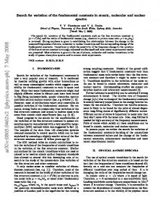
On much shorter timescales, several tests using frequency standards have been performed [9, 10, 11]. These laboratory tests have a very high sensitivity to changes in fundamental constants. They are repeatable, systematic errors can be tracked as experimental conditions can be changed. In this letter we present results that place a new stringent limit to the time variation of fundamental constants. By comparing the hyperfine energies of 133 Cs and 87 Rb in their electronic ground state over a period of nearly five years, we place an upper limit to the rate of change of the ratio of the hyperfine frequencies νRb /νCs . Our measurements take advantage of the high accuracy (∼ 10−15 ) of several laser cooled Cs and Rb atomic fountains. According to recent atomic structure calculations [11, 12], these measurements are sensitive to a possible variation of the quantity (µRb /µCs )α−0.44 , where µ’s are the nuclear magnetic moments. We anticipate major advances in these tests using frequency standards, thanks to recent advances in optical frequency metrology using femtosecond lasers [13, 14]. In our experiments, three atomic fountains are compared to each other, using a hydrogen maser (H-maser) as a flywheel oscillator (Fig.1). Two fountains, a transportable fountain FOM, and FO1 [15] are using cesium atoms. The third fountain is a dual fountain (DF) [16], operating alternately with rubidium (DFRb ) and cesium (DFCs ). These fountains have been continuously upgraded in order to improve their accuracy from 2 × 10−15 in 1998 to 8 × 10−16 for cesium and from 1.3 × 10−14 [17] to 6 × 10−16 for rubidium. Fountain clocks operate as follows. First, atoms are collected and laser cooled in an optical molasses or in a magneto-optical trap in 0.3 to 0.6 s. Atoms are launched upwards, and selected in the clock level (mF = 0) by a combination of microwave and laser pulses. Then, atoms interact twice with a microwave field tuned near the

2

F O 1

H -m a s e r

D F

FOM

Maser Fractional

Frequency Offset (10

-15

)

Rb

285

DF

FIG. 1: BNM-SYRTE clock ensemble. A single 100 MHz signal from a H-maser is used for frequency comparisons and is distributed to each of the microwave synthesizers of the 133 Cs (FO1, FOM, DFCs ) and 87 Rb fountain clocks. In 2001, the Rb fountain has been upgraded and is now a dual fountain using alternately rubidium (DFRb ) or cesium atoms (DFCs ).

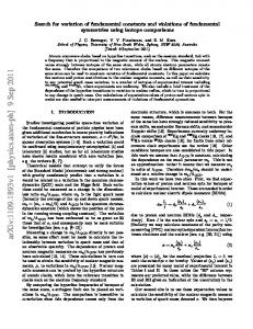
The three fountains have different geometries and operating conditions: the number of detected atoms ranges from 3 × 105 to 2 × 106 at a temperature of ∼ 1 µK, the fountain cycle duration from 1.1 to 1.6 s. The Ramsey resonance width is between 0.9 and 1.2 Hz. In measurements reported here the fractional frequency instability is (1 − 2) × 10−13 τ −1/2 , where τ is the averaging time in seconds. Fountain comparisons have a typical resolution of ∼ 10−15 for a 12 hour integration, and each of the four data campaigns lasts from 1 to 2 months during which an accuracy evaluation of each fountain is performed. The 2002 measurements are presented in Fig.2, which displays the maser fractional frequency offset, measured by the Cs fountains FOM and DFCs . Also shown is the H-maser frequency offset measured by the Rb fountain DFRb where the Rb hyperfine frequency is conventionally chosen to be νRb (1999) = 6 834 682 610.904 333 Hz, our 1999 value. The data are corrected for the systematic frequency shifts listed in Table I. The H-maser frequency exhibits fractional fluctuations on the order of 10−14 over a few days, ten times larger than the typical statistical uncertainty resulting from the instability of the fountain clocks. In order to reject the H-maser frequency fluctuations, the fountain data are recorded simultaneously (within a few minutes). The fractional frequency differences plotted in Fig.2 b illustrate the efficiency of this

Cs

280

275

270

265

-15

)

260

10

b)

5 0 -5 -10 52560

C s

F O M

a)

DF

difference (10

R b C lo c k s

290

Fractional frequency

hyperfine frequency, in a Ramsey interrogation scheme. The microwave field is synthesized from a low phase noise 100 MHz signal from a quartz oscillator, which is phase locked to the reference signal of the H-maser (Fig.1). After the microwave interactions, the population of each hyperfine state is measured using light induced fluorescence. This provides a measurement of the transition probability as a function of microwave detuning. Successive measurements are used to steer the average microwave field to the frequency of the atomic resonance using a digital servo system. The output of the servo provides a direct measurement of the frequency difference between the H-maser and the fountain clock.

52570

52580

52590

52600

Date (MJD)

FIG. 2: The 2002 frequency comparison data. a) H-maser fractional frequency offset versus FOM (), and alternately versus DFRb (◦) and DFCs (△ between dotted lines). b) Fractional frequency differences. Between dotted lines, CsCs comparisons, outside Rb-Cs comparisons. Error bars are purely statistical. They correspond to the Allan standard deviation of the comparisons and do not include contributions from fluctuations of systematic shifts of Table I.

rejection. DF is operated alternately with Rb and Cs, allowing both Rb-Cs comparisons and Cs-Cs comparisons (central part of Fig.2) to be performed. TABLE I: Accuracy budget of the fountains involved in the 2002 measurements (DF et FOM). Fountain

DFCs

DFRb

FOM

Effect Value & Uncertainty (10−16 ) 2nd order Zeeman 1773.0 ± 5.2 3207.0 ± 4.7 385.0 ± 2.9 Blackbody Radiation −173.0 ± 2.3 −127.0 ± 2.1 −186.0 ± 2.5 Cold collisions −95.0 ± 4.6 0.0 ± 1.0 −24.0 ± 4.8 + cavity pulling others 0.0 ± 3.0 0.0 ± 3.0 0.0 ± 3.7 Total uncertainty 8 6 8

Systematic effects shifting the frequency of the fountain standards are listed in Table I. The quantization magnetic field in the interrogation region is determined with a 0.1 nT uncertainty by measuring the frequency of a linear field-dependent “Zeeman” transition. The temperature in the interrogation region is monitored with 5 platinum resistors and the uncertainty on the blackbody radiation frequency shift corresponds to temperature fluctuations of about 1 K [18]. Clock frequencies

3

DF FOM νCs (2002) − νCs (2002) = +12(6)(12) × 10−16 νCs

(1)

where the first parenthesis reflects the 1σ statistical uncertainty, and the second the systematic uncertainty, obtained by adding quadratically the inaccuracies of the two Cs clocks (see Table I). The two Cs fountains are in good agreement despite their significantly different operating conditions (see Table I), showing that systematic effects are well understood at the 10−15 level. In 2002, the 87 Rb frequency measured with respect to the average 133 Cs frequency is found to be: νRb (2002) = 6 834 682 610.904 324(4)(7) Hz

(2)

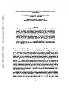
where the error bars now include DFRb , DFCs and FOM uncertainties. This is the most accurate frequency measurement to date. In Fig.3 are plotted all our Rb-Cs frequency comparisons. Except for the less precise 1998 data [17], two Cs fountains were used together to perform the Rb measurements. The uncertainties for the 1999 and 2000 measurements were 2.7 × 10−15 , because of lower clock accuracy and lack of rigorous simultaneity in the earlier frequency comparisons [16]. A weighted linear fit to the data in Fig.3 determines how our measurements constrain a possible time variation of νRb /νCs . We find:   νRb d = (0.2 ± 7.0) × 10−16 yr−1 (3) ln dt νCs which represents a 5-fold improvement over our previous results [16] and a 100-fold improvement over the Hg+ -H hyperfine energy comparison [11]. We now examine how this result constrains possible variations of fundamental constants. For an alkali with atom number Z, the hyperfine transition frequency can be approximated by:   me µ R∞ c Frel (Zα), (4) ν ∝ α2 µN mp

MJD 50500

51000

51500

52000

52500

53000

-15

)

10

Fractional frequency (10

are corrected for the cold collision and cavity pulling frequency shifts using several methods [19, 20]. All other effects do not contribute significantly and their uncertainties are added quadratically. We searched for the influence of synchronous perturbations by changing the timing sequence and the atom launch height. To search for possible microwave leakage, we changed the power (×9) in the interrogation microwave cavity. No shift was found at a resolution of 10−15 . The shift due to residual coherences and populations in neighboring Zeeman states is estimated to be less than 10−16 . As shown in [21], the shift due to the microwave photon recoil is very similar for Cs and Rb and smaller than +1.4 × 10−16 . Relativistic corrections (gravitational redshift and second order Doppler effect) contribute to less than 10−16 in the clock comparisons. For the Cs-Cs 2002 comparison, we find:

5

0

-5

-10

-15

-20

1997

1998

1999

2000

2001

2002

2003

2004

Year

FIG. 3: Measured 87 Rb frequencies referenced to the 133 Cs fountains over 57 months. The 1999 measurement value (νRb (1999) = 6 834 682 610.904 333 Hz) is conventionally used as reference. A weighted linear fit to the data gives   νRb d ln νCs = (0.2 ± 7.0) × 10−16 yr−1 . Dotted lines corredt spond to the 1σ slope uncertainty.

where R∞ is the Rydberg constant, c the speed of light, µ the magnetic moment of the nucleus, µN the nuclear magneton. Frel (Zα) is a relativistic function which strongly increases with Z [11, 22]. For 133 Cs, this Casimir relativistic contribution amounts to 40 % of the hyperrel (Zα)) fine splitting and α ∂ln(F∂α = 0.74. For 87 Rb, this quantity is 0.30 [27]. Following [11] and neglecting possible changes of the strong and weak interactions affecting µRb and µCs , the sensitivity of the ratio νRb /νCs to a variation of α is simply given by:   νRb ∂ ≃ (0.30 − 0.74) = −0.44. (5) ln ∂ ln α νCs Using equations 3 and 5, we thus set the new limit: α/α ˙ = (−0.4 ± 16) × 10−16 yr−1 . In contrast with [11], Ref.[22] argues that a time variation of the nuclear magnetic moments must also be considered in a comparison between hyperfine frequencies. The magnetic moments µ can be calculated using the Schmidt model. For atoms with odd A and Z such as 87 Rb and 133 Cs, the Schmidt magnetic moment µ(s) is found to depend only on gp , the proton gyromagnetic ratio. With this simple model, Ref.[22] finds: !   (s) µRb ∂ νRb ∂ ≃ 2.0. (6) ≃ ln ln (s) ∂ ln gp νCs ∂ ln gp µ Cs

Attributing any variation of νRb /νCs to a variation of gp , equations 3 and 6 lead to: g˙p /gp = (0.1 ± 3.5) × 10−16 yr−1 . However, it must be noted that the Schimdt model is over simplified and does not agree very accurately with the actual magnetic moment.

4 Moreover, attributing all the time variation of νRb /νCs to either gp or α independently is somewhat artificial. Theoretical models allowing for a variation of α also allow for variations in the strength of the strong and electroweak interactions. For instance, Ref.[5] argues that Grand unification of the three interactions implies that a time variation of α necessarily comes with a time variation of the coupling constants of the other interactions. Ref.[5] predicts that a fractional variation of α is accompanied with a ∼ 40 times larger fractional change of me /mp . In order to independently test the stability of the three fundamental interactions, several comparisons between different atomic species and/or transitions are required. For instance and as illustrated in [14], absolute frequency measurements of an optical transition is sensitive to a different combination of fundamental constants: (µCs /µN )(me /mp )αx , where x depends on the particular atom and/or transition. A more complete theoretical analysis going beyond the Schmidt model would clearly be very useful to interpret frequency comparisons involving hyperfine transitions. This is especially important as most precise frequency measurements, both in the microwave and the optical domain [14, 23, 24], are currently referenced to the 133 Cs hyperfine splitting, the basis of the SI definition of the second. The H hyperfine splitting, which is calculable to a high accuracy, has already been considered as a possible reference several decades ago. Unfortunately, despite numerous efforts, the H hyperfine splitting is currently measured to only 7 parts in 1013 (using H-masers), almost three orders of magnitude worse than the results presented in this letter. In summary, by comparing 133 Cs and 87 Rb hyperfine energies, we have set a stringent upper limit to a possible fractional variation of the quantity (µRb /µCs )α−0.44 at (−0.2 ± 7.0) × 10−16 yr−1 . In the near future, accuracies near 1 part in 1016 should be achievable in microwave atomic fountains, improving our present Rb-Cs comparison by one order of magnitude. We anticipate that comparisons between rapidly progressing optical and microwave laser-cooled frequency standards currently developed in several laboratories will bring orders of magnitude gain in sensitivity. In order to have the full benefit of these advances, frequency comparisons with improved accuracy between these distant clocks will be necessary. Serving this purpose, a new generation of time/frequency transfer at the 10−16 level is currently under development for the ESA space mission ACES which will fly ultra-stable clocks on board the international space station in 2006 [25]. These comparisons will also allow for a search of a possible change of fundamental constants induced by the annual modulation of the Sun gravitational potential due to the elliptical orbit of the Earth [26]. The authors wish to thank T. Damour, J.P. Uzan, and P. Wolf for valuable discussions, A. G´erard and the elec-

tronic staff for technical assistance. This work was supported in part by BNM, CNRS and CNES. BNM-SYRTE and Laboratoire Kastler Brossel are Unit´es Associ´ees au CNRS, UMR 8630 and 8552.

∗

†

[1] [2] [3] [4]

[5] [6] [7] [8] [9] [10] [11] [12] [13]

[14] [15] [16]

[17] [18] [19] [20] [21] [22] [23] [24] [25] [26] [27]

Present address: Istituto Elettrotecnico Nazionale G. Ferraris , Strada delle Cacce 41, 10135 Torino, Italy Present address: Institutul National de Fizica Laserilor, Plasmei si Radiatiei, P.O. Box MG36, Bucaresti, Magurele, Romania P.A.M. Dirac, Nature 139, 323 (1937). F. Dyson, in Current trends in the theory of fields, (AIP New-York, 1983), p. 163. For a review, see for instance J.P. Uzan, ArXiv: hepph/0205340, and references therein. T. Damour and A. Polyakov, Nucl. Phys. B 423, 532 (1994); T. Damour, F. Piazza, and G. Veneziano, Phys. Rev. Lett. 89, 081601 (2002). X. Calmet and H. Fritzsch, Eur. Phys. J. C 24, 639 (2002). T. Damour and F. Dyson, Nucl. Phys. B 480, 37 (1996). A.V. Ivanchik, E. Rodriguez, P. Petitjean and D.A. Varshalovich, Astron. Lett. 28, 423 (2002). J.K. Webb et al., Phys. Rev. Lett. 87, 091301 (2001). J.P. Turneaure et al., Phys. Rev. D 27, 1705 (1983). A. Godone, C. Novero, P. Tavella and K. Rahimullah, Phys. Rev. Lett. 71, 2364 (1993). J.D. Prestage, R.L. Tjoelker and L. Maleki, Phys. Rev. Lett. 74, 3511 (1995). V.A. Dzuba, V.V. Flambaum and J.K. Webb, Phys. Rev. A 59, 230 (1999). See for instance Proc. of the 6th Symposium on Frequency Standards and Metrology (World Scientific, Singapore, 2001). S. Bize et al., submitted to Phys. Rev. Lett, (2002). A. Clairon et al., in Proc. of the 5th Symposium on Frequency Standards and Metrology, ed. J. Bergquist (World Scientific, Singapore, 1995), p. 49. S. Bize et al., in Proc. of the 6th Symposium on Frequency Standards and Metrology (World Scientific, Singapore, 2001), p 53. S. Bize et al., Europhys. Lett. 45, 558 (1999). E. Simon et al., Phys. Rev. A 57, 436 (1998). F. Pereira Dos Santos et al., Phys. Rev. Lett. 89, 233004 (2002). Y. Sortais et al., Phys. Rev. Lett. 85, 3117 (2000). P. Wolf et al., in Proc. of the 6th Symposium on Frequency Standards and Metrology (World Scientific, Singapore, 2001), p 593. S.G. Karshenbo¨ım, Can. J. Phys. 47, 639 (2000). M. Niering et al., Phys. Rev. Lett. 84, 5496 (2000). Th. Udem et al., Phys. Rev. Lett. 86, 4996 (2001). C. Salomon et al., C. R. Acad. Sci. Paris, t.2, S´erie IV, 1313 (2001). A. Bauch and S. Weyers, Phys. Rev. D 65, 081101 (R) (2002). A more precise calculation in [12] gives LdFrel (133 Cs) = 0.83, which differs by 10% from the Casimir formula.