19th International Congress on Modelling and Simulation, Perth, Australia, 12–16 December 2011 http://mssanz.org.au/modsim2011
A Semi-Ordered Fast Iterative Method (SOFI) for Monotone Front Propagation in Simulations of Geological Folding T. Gillberg a , a
Computational Geosciences, Simula Research Laboratory, P.O. Box 134, 1325 Lysaker, Norway Email:
[email protected]
Abstract: This paper present a novel algorithm for monotone front propagation of anisotropic nature. In several examples the new algorithm is shown to be fast and able to solve a general class of front propagation problems. The algorithm is inspired by Huygens’ principle in that the front is described using a list of nodes that are used as source points to evolve the front. Nodes affected by the source points are either directly used as source points or temporarily paused, depending on their solution value and the average solution value of all source points. This feature makes the algorithm semi-ordered. Still, nodes may be used as source points several times, making the algorithm iterative of nature. Together, these features create the Semi-Ordered Fast Iterative (SOFI) method. Unlike other iterative algorithms the performance does not depend strongly on the domain geometry or variations in front velocity. Instead, the performance seems closer to that of the more stable Ordered Upwind Methods. We compare the computational time between the SOFI and Fast Marching method for an increasing grid on two isotropic examples. The computational time of the SOFI method is shorter than that of the Fast Marching method, especially on large grids. Ordered Upwind Methods have a computational scaling of O(N log N ), where N is the total number of unknown nodes. The log N factor stems from the sorting needed for the front propagation. The SOFI method needs no sorting, and our numerical experiments indicate that it is of order O(N ). On isotropic examples the SOFI method solutions are identical to those from the Fast Marching method assuming the same stencil is used in both methods. On problems with anisotropy the solutions are identical to those from the Fast Sweeping method when the same stencils are used. The SOFI method has many similarities with two recently introduced iterative methods, the Fast Iterative method and the Two Queue method. The Fast Iterative method lacks the semi-ordering, and its performance is therefore very problem dependent. The Two Queue method also pauses nodes to get a partially ordered method, but is only applicable to isotropic problem formulations. Stencils of different forms can be used with minor modifications of the algorithm. We present examples where the stencil uses only edge connected nodes, and also when diagonal nodes are included in the stencil. The SOFI method can use any consistent local wave approximation (stencil), and may therefore keep the constant velocity assumption to a small area unlike the Ordered Upwind Methods which often assume that the velocity profile is constant in a larger neighbourhood. In geoscience, the simulation of an expanding front is used for the modelling of structural folds. Modelling of geological folding is a key component of the shared earth model the Compound Earth Simulator, developed by the oil and gas company Statoil. Non-parallel folds are modelled using anisotropic front propagation, where the velocity of the front depends on the direction the front is moving. Three different classes of folds are illustrated in our example section, all created using the SOFI method. Keywords: Monotone front propagation, geological folding, static Hamilton-Jacobi equations, the Eikonal equation.
641
T. Gillberg, SOFI; A Semi-Ordered Fast Iterative method for anisotropic front propagation 1
I NTRODUCTION
The simulation of an expanding front is needed in many scientific applications. In the Earth sciences fast solutions are used in forward modelling of seismic data (Rawlinson and Sambridge (2004)), to describe complex folding structures in geological systems (Hjelle and Petersen (2011)), and in reservoir simulations (Berre et al. (2005)).There are many applications in other fields discussed by Sethian (1999), including grid generation, optimal path planning, and computer visualisation applications. Statoil is currently developing a shared earth model; the Compound Earth Simulator or for short Compound. The Compound framework models an earth segment by combining drill measurements and seismic data with human intuition. A user can restore faults and folded structures interactively, and furthermore simulate the geological evolution by placing geological events and processes along a timeline. A key component in Compound is the modelling of geological folds as described in Hjelle and Petersen (2011). To obtain a user-friendly and interactive application the simulations must be fast and accurate. Both speed and accuracy can be increased by using an alternative stencil formulation that include nodes diagonal to the point being updated (Gillberg et al. (2011)). 2
BACKGROUND
In this section we briefly discuss a mathematical framework for monotone front propagation, and two concepts of importance to our algorithm design. Front Propagation. The expanding front is described by its (first) time of arrival, T , to all points in a domain Ω from the start position Γ. A general mathematical framework for the time-of-arrival is given by static Hamilton-Jacobi equations of the form H(x, ∇T ) = 0, T (x) = 0 ∀x ∈ Γ,
(1)
where H is convex in ∇T . The solution T (x) can be thought of as the distance from x to Γ, as measured 1 with a metric defined by H. Solutions to the Eikonal equation H(x, ∇T ) = ∇T · ∇T − F (x) 2 with F ≡ 1, is the minimal Euclidian distance from x to Γ. Causality. What lies ahead of a moving front does not affect the past movements of the front. This property is known as the causality principle. For monotone front propagation causality states that smaller values do not depend on larger ones. Causality implies that the solution should be constructed in an increasing order, an approach heavily exploited by several algorithms, know as front tracking methods. On a discrete setting the causality principle cannot be directly employed, since larger valued nodes may affect the solution of smaller ones. This is due to the way the front is modelled in the update step, that is the numerical stencils. All stencils use some sort of interpolation of values between nodes. However, for an upwind-stencil we can formulate the following discrete causality principle. The value at node D, TD , is to be approximated using solution values to nodes of the set {U1 , . . . , Un }. Observation 1. The value at D might depend on the values of {U1 , . . . , Un } only if
min
{U1 ,...,Un }
TUi < TD .
If min TUi i=1,...,n ≥ TD then node D is upwind (behind) all of U1 , . . . , Un , and the front will first pass node D and later nodes U1 , . . . , Un . If Ui < TD for some i, then node D is downwind of Ui , and the time the front reaches D may depend on the time the front first reached Ui , and therefore {U1 , . . . , Un }. Observation 1 is a weak, but very general, discrete formulation of the causality principle that is valid for any upwind finite difference stencil for front propagation. With a given stencil and propagation formulation it is often possible to come up with a stricter discrete causality formulation, as done for the Eikonal equation in Gillberg et al. (2011). Huygens’ principle. Huygens’ principle is formulated as follows by Alton (2010): All points on a wavefront serve as point sources of secondary wavelets. After a short time the new position of the wavefront will be that of the surface tangent to those secondary wavelets. Instead of following the entire front continuously, one can look at the front as described by a set of source points. The combined front (envelope) of all source points gives the new front position. In short, the
642
T. Gillberg, SOFI; A Semi-Ordered Fast Iterative method for anisotropic front propagation method presented in section 4 is a discrete version of Huygens’ principle, which traces the front using the mean solution value of the discrete source points. 3
F RONT P ROPAGATION A LGORITHMS
The algorithms that exploit the causality principle the most are the front tracking methods, such as the Fast Marching and Expanding Wavefront Methods, presented by Sethian (1999) and Qin et al. (1992). Front tracking methods approximate the front, and use the point on the front with minimal value as a source point to further evolve the front, before considering the point as passed by the front. Since a node is only passed one time, these algorithms are called one-pass methods. In order to know which node is to be passed next, an ordered data structure is needed. Therefore, parallel implementations of these algorithms are difficult to achieve. The method can be made faster by passing a set of nodes close to the wave front simultaneously as suggested by Kim (2001). Extensions to anisotropic propagation are known as Ordered Upwind Methods. These methods are complicated, some must be simplified to be implemented, and need prior knowledge of the degree of anisotropy in the problem, see for instance Cristiani (2009); Vladimirsky (2003); Alton (2010). The Ordered Upwind methods use a large neighbourhood when updating a node. By doing so, an underlying assumption is that the velocity is constant in the larger neighbourhood, which is not the case for problems with local anisotropy. Another approach is to sweep the front in a set of predefined directions with Gauss-Seidel iterations, see Qian et al. (2007), or by assuming the front will have a spherical-like shape as done by Vidale (1988). These iterative methods are sensitive to domain geometry and variations in the velocity, and are therefore often slower than front tracking methods. Complex domain geometries and velocity variations may cause the solution dependencies, the characteristic curves, to twist and bend and many iterations are often needed. Recently, two iterative algorithms that make partial use of the causality principle have been presented, the Fast Iterative method by Jeong and Whitaker (2008), and the Single/Two Queue methods by Bak et al. (2010). The Fast Iterative and Single Queue methods have an active list (queue) of nodes to expand the wave everywhere simultaneously, and their performance is highly problem dependent. The Two Queue method enforces a better use of causality, and is therefore less problem dependent than the Fast Iterative and Single Queue methods. The Queue methods need fewer operations than the Fast Iterative method, but they are only capable to solve isotropic front propagation problems. 4
T HE S EMI -O RDERED FAST I TERATIVE M ETHOD
Let ΩD denote the set of nodes on which we wish to compute the time of arrival, and assume that the initial distance is known at the nodes ΓD ⊂ ΩD . Initially, we assume that the front does not reach any nodes that are not initialised, T (x) = ∞ ∀x ∈ ΩD \ ΓD . The current front is described by a list, aL, containing source points (active nodes). In the initialisation step, all initialised nodes are added to aL. We also have a list of nodes who are ahead of the source points, pL, that initially is empty but later will contain paused nodes, that is nodes that later will be used as source points. As in Huygens’ interpretation of a moving front, all nodes in aL are used as source points to evolve the front. Using observation 1, close nodes potentially downwind of a source point are updated using stencils where the source point is included. In the observation, U1 , . . . , Un are all nodes in the stencil, and D is the close node. The definition of close nodes depends on the stencil form. For example if the stencil only uses edge connected nodes (bottom stencil of figure 1(b)) only edge connected neighbours to the source point need to be updated. If the stencil uses both edge and diagonal neighbours on a regular grid (top stencil figure 1(b)), the diagonal nodes of the source point may also need to be updated. These corresponding stencil forms will be referred to as a diagonal and edge stencil respectively. The diagonal stencil is the more accurate since it makes use of a more local wave approximation, see Gillberg et al. (2011) for details. We construct the solution in a semi-ordered fashion using a parameter av. Assume that node xn receives a new solution value that is smaller than the old value, t < T (xn ). If in addition t ≤ av then xn is added to the end of aL, and used as a source point. If instead t > av, we postpone its function as a source by adding xn to pL. The approach of using two lists was first suggested by Glover et al. (1985). Let mk be the average solution value of all nodes added to pL during iteration k − 1 of the aL list. By choosing
643
T. Gillberg, SOFI; A Semi-Ordered Fast Iterative method for anisotropic front propagation
(a) SOFI pseudo code
(b) Diagonal and edge stencil forms
Figure 1: (a) Pseudo code for the SOFI method. (b) Two stencil forms, where the arrow points to the node being updated. Top shows a diagonal stencil, and bottom an edge stencil.
av = mk we enforce causality with no prior information of the problem. The method may benefit by relaxing the semi-ordering by choosing av = 1.3mk − 0.3mk−1 1 . The relaxation is beneficial if an edge stencil is used but not noticeably when a diagonal stencil is used. When there are no source points left, no nodes in ΩD can get a lower arrival time. Any upwind stencil with a proper upwind condition can be applied if the source point neighbours are correctly defined. Figure 1(a) shows pseudo code for SOFI. 5
N UMERICAL V ERIFICATION
If the stencil uses diagonally connected nodes, nodes diagonal of the source point should be updated. However, when not mentioned otherwise, the semi-ordering of SOFI assures a correct solution with only edge connected updates on the examples in this section. In case of highly irregular speed functions, or strong anisotropy, the diagonal update should be included to get solutions with the smallest errors. 5.1
Computational order and the Hamilton-Jacobi-Bellman equation
In order to illustrate the computational order, graphs in figures 2(a) and 2(b) show CPU times for an increasing number of nodes for both the Fast Marching and SOFI methods applied to two isotropic problems. Both methods has been implemented in C++, compiled with O3 optimization, and uses identical stencil formulations. Solid (dashed) lines are CPU times for the SOFI method with a diagonal (edge) stencil, and dotted (dash-dotted) lines are CPU times for the Fast Marching method with a diagonal (edge) stencil. All computational times are averages of 5 runs on a MacBookPro with a 2.66 GHz Intel Core 2 Duo processor and 2 × 2 GB 1067 MHz DDR3 ram memory. The two equations which are solved are k∇T k = 1,
T (50, 50) = 0,
0 ≤ x, y ≤ 100
(2)
k∇T k q = 1, 2 100 sin y 2 sin x2 + (1.01 + cos x cos y)
T (x, 0) = 0,
0 ≤ x, y ≤ 10.
(3)
The characteristic curves of (2) are straight lines, but they are curved for (3) which indicates that iterative methods perform badly. For a given stencil the SOFI method is 2.4-4.8 times faster depending on grid 1 Approximately
50% of the nodes are activated with no relaxation. Bak et al. (2010) suggest that 65–75% are optimal.
644
T. Gillberg, SOFI; A Semi-Ordered Fast Iterative method for anisotropic front propagation
(a) CPU time, distance to centered point
(b) CPU time, complex isotropic speed
(c) Five 5-isocurves to (4)
Figure 2: (a) and (b) show the computational time in seconds for the total number of nodes for (2) and (3). Solid (dashed) lines are CPU times for the SOFI method with a diagonal (edge) stencil, dotted (dash-dot) lines are CPU times for the Fast Marching method with a diagonal (edge) stencil. Figure (c) shows the 5-isocurve for five solutions with different anisotropic directions of (4).
sizes for (2). For the more complex problem of (3), the computations of the velocity are very time consuming, and the SOFI method is therefore only 1.1-2.2 times faster. Notice that the diagonal stencil is faster for both methods, supported by Gillberg et al. (2011). The Fast Marching method has a computational scaling of O(N log N ), visible especially on the simple distance computation. There is no sorting in the SOFI method, and every source point has a constant number of neighbour nodes. Together with figures 2(a) and 2(b), these observations implies a computational scaling of O(N ) for the SOFI method. The SOFI method solution is identical to the Fast Marching solution for both equations. We counted the average number of stencil solves per node for these isotropic problems on a grid of 560×560 nodes. For equation (2) the SOFI method needs 1.996 updates for both stencil types, precisely the same number as the Fast Marching method. The Two Queue method need 1.626, and the Single Queue method only 1, update per node (Bak et al. (2010)). The performance for problem (3) is very different. Here the SOFI method with a diagonal stencil use 2.047, and with an edge stencil 2.906 stencil solves. The Fast Marching method need on average 1.998 updates for both stencil types. The Single Queue method need 186.863, and the Two Queue method with dynamic queue cutoff 2.312 updates per node. A significant drawback for the Two Queue methods is that the average speed is needed for the cutoff implementation. The average speed can be both costly and difficult to compute. Our first anisotropic example is of Hamilton Jacobi Bellman type, describing the distance from a point in a tilted plane, z = c1 x + c2 y. The problem is formulated by min
u∈B 2
(∇T (x) · −u) = 1, 0 ≤ x, y ≤ 1, T (0.5, 0.5) = 0, (1 + (c · u)2 )1/2
(4)
where B 2 is the set of all unit vectors. On a discrete setting the causality principle cannot be directly employed, since larger valued nodes may affect the solution of smaller ones. Therefore (4) cannot be solved by a Fast Marching approach (Cristiani (2009); Vladimirsky (2003)). √ iπ Figure 2(c) shows the 5-isocurve for solutions to (4) with c = 10(sin iπ 5 , cos 5 ) for i = 1, 2, 3, 4, 5, created on a grid of 101×101 nodes. The used stencils are of diagonal form. In the update step the stencil including the smaller diagonal node is first solved, and thereafter the stencil including the larger diagonal node is considered. The average number of updates per node if only edge neighbours are updated are 5.206 per node. If also nodes diagonal from the source point are included the average number of operations increases to 7.415. The degree of anisotropy, as described in√Vladimirsky (2003), for this p √ problem is 1 + |c|2 = 11. If we increase the degree of anisotropy to 21, diagonal nodes from the source should be updated to get a solution with the smallest errors. The number of operations per node then increases to 10.952. The solution of these examples are identical to that of the Fast Sweeping method if the same stencils are used, and numerical convergence estimates for similar anisotropic equations are presented in Qian et al. (2007).
645
T. Gillberg, SOFI; A Semi-Ordered Fast Iterative method for anisotropic front propagation
(a) Fold of class 1A
(b) Fold of class 1B (parallel)
(c) Fold of class 1C
Figure 3: Three modelled folds of different classes, from left class 1A, 1B, 1C after Ramsay’s classification system, as explained in Hjelle and Petersen (2011). The initial horizon, marked with red, and the anisotropic direction, a = (−0.2, 1.0), is the same in all figures. Negative and positive contour lines are dashed and solid respectively.
5.2
Fold Modelling
Modelling of geological folding is an important component in the Compound Earth Simulator. For this purpose Hjelle and Petersen (2011) developed a mathematical framework that takes an horizon as initial condition and simulates a folded structure in a given domain. This framework can replicate all fold classes as defined by Ramsay (1967) by changing parameter values of F and ψ in the equation F k∇T k + ψ (a · ∇T ) = 1.
(5)
Here, a defines the axial direction of the fold. Interestingly, the characteristic curves to (5) coincide with the dip-isogons often used for classifications of folded structures. A minor extension of the algorithm is needed, since the folded structures above and below the initial horizon have a positive and negative axial direction respectively. This feature is modelled by propagating a sign with the front. The Fast Marching method does not create the correct solution for any but the parallel folding class, where ψ = 0. Figure 3 shows three folds from the same initial horizon (shown in red) where the dashed lines are negative isocurves, and solid lines positive. All folds in figure 3 have the axial direction a = (−0.2, 1), and are simulated on a fine grid of 401×401 nodes. For the class 1A fold in figure 3(a) we have F = 1, ψ = −0.5, for the class 1B (parallel) fold in figure 3(b) we have F = 1, ψ = 0, and for the class 1C fold of figure 3(c) we have F = 1, ψ = 1. The remaining fold classes 2 and 3 are modelled with F = 0, ψ > 0, and F < 0, ψ > 0, respectively. 5.3
Conclusions
We presented a new Semi-Ordered Fast Iterative algorithm for monotone front propagation. The SOFI method is fast and simple to implement, and works for general anisotropic front propagations. Unlike other iterative algorithms, the performance does not depend strongly on the variations of the speed, but somewhat on the degree of anisotropy. Instead, the performance of SOFI is more similar to the class of Ordered Upwind Methods, but no prior information on the degree of anisotropy or simplification of the algorithm are needed. For the SOFI method, numerical experiments indicate a computational scaling of degree O(N ), where N is the total number of unknown nodes. Regarding accuracy, the SOFI method has an identical solution to the Fast Marching method for isotropic equations, and as the Fast Sweeping method for anisotropic problems, when the methods has identical stencil formulations. The SOFI method can use any consistent local wave approximation (stencil), and may therefore keep the constant velocity assumption to a small area. On isotropic examples the proposed method was shown to be very fast compared to the Fast Marching method. This relation hods for both the more accurate diagonal stencil form, and the edge stencil. Huygens’ principle implies that source points on the front that are
646
T. Gillberg, SOFI; A Semi-Ordered Fast Iterative method for anisotropic front propagation not close to each other are independent of each other, thus implying parallel implementation possibilities of the SOFI method. However, there is a communication problem when different source points on different processors try to update the same node, most likely requiring a domain decomposition approach. Continuation of this work will compare the performance of the algorithm in three dimensions to the performance of other popular approaches, and further test efficiency of the method on anisotropic problems. It would also be interesting to test the algorithm on non-rectangular grids, where the method itself is directly applicable. Within seismic processing the computational time is often very long. Therefore the SOFI method is a promising alternative for simulating seismic traveltimes fast. ACKNOWLEDGEMENT The author is very thankful to the anonymous reviewers who help to improve the paper. The presented work was funded by Statoil through the Akademia program, and the Research Council of Norway under grant 202101/I40. The work has been conducted at Kalkulo AS, a subsidiary of Simula Research Laboratory. R EFERENCES Alton, K. (2010). Dijkstra-like Ordered Upwind Methods for Solving Static Hamilton-Jacobi Equations. Ph. D. thesis. Bak, S., J. McLaughlin, and D. Renzi (2010). Some improvements for the fast sweeping method. SIAM Journal on Scientific Computing 32, 2853. Berre, I., K. H. Karlsen, K.-A. Lie, and J. R. Natvig (2005, November). Fast computation of arrival times in heterogeneous media. Computational Geosciences 9(4), 179–201. Cristiani, E. (2009). A fast marching method for Hamilton-Jacobi equations modeling monotone front propagations. Journal of Scientific Computing 39(2), 189–205. Gillberg, T., Ø. Hjelle, and A. M. Bruaset (2011). Accuracy and efficiency of stencils for the eikonal equation in earth modelling. Submitted. Glover, F., D. Klingman, and N. Phillips (1985, January). A new polynomially bounded shortest path algorithm. Operations Research 33(1), 65–73. Hjelle, Ø. and S. A. Petersen (2011). A Hamilton-Jacobi framework for modeling folds in structural geology. Mathematical Geosciences, 1–21. Jeong, W.-K. and R. T. Whitaker (2008). A fast iterative method for eikonal equations. SIAM Journal on Scientific Computing 30(5), 2512–2534. Kim, S. (2001). An O(N ) level set method for eikonal equations. SIAM Journal on Scientific Computing 22(6), 2178–2193. Qian, J., Y. Zhang, and H. Zhao (2007, March). A fast sweeping method for static convex HamiltonJacobi equations. Journal of Scientific Computing 31(1-2), 237–271. Qin, F., Y. Luo, K. B. Olsen, W. Cai, and G. T. Schuster (1992). Finite-difference solution of the eikonal equation along expanding wavefronts. Geophysics 57(3), 478–487. Ramsay, J. G. (1967). Folding and fracturing of rocks. McGraw-Hill, New York and London. Rawlinson, N. and M. Sambridge (2004). Multiple reflection and transmission phases in complex layered media using a multistage fast marching method. Geophysics 69(5), 1338–1350. Sethian, J. A. (1999). Level Set Methods and Fast Marching Methods. Cambridge University Press. Vidale, J. (1988). Finite-difference calculation of travel times. Bulletin of the Seismological Society of America 78(6), 2062. Vladimirsky, A. (2003). Ordered upwind methods for static Hamilton-Jacobi equation: Theory and algorithms. SIAM Journal of Numerical Analysis 41(1), 325.
647