MATERIALS FORUM VOLUME 33 - 2009 Edited by Dr Steve Galea, Associate Professor Wingkong and Professor Akira Mita © Institute of Materials Engineering Australasia Ltd
A SENSOR-BASED LEARNING APPROACH TO PROGNOSTICS IN INTELLIGENT VEHICLE HEALTH MONITORING I. S. Cole*1, P. A. Corrigan1, G. C. Edwards2, D. Followell3, S. Galea4, W. Ganther1, B. R. Hinton4, T. Ho1, C. J. Lewis2, T. H. Muster1, D. Paterson1, D. C. Price2, D. A. Scott2, P. Trathen4. 1
4
CSIRO Materials Science and Engineering, Gate 5 Normanby Road, Clayton, Vic., 3168, Australia. 2 CSIRO Materials Science and Engineering, P.O. Box 218, Lindfield, NSW, Australia. 3 Boeing Phantom Works, St. Louis, MO, USA. Defence Science and Technology Organisation, 506 Lorimer Street, Fishermans Bend, Vic., 3207, Australia. * Corresponding author email:
[email protected]
ABSTRACT This paper outlines recent progress towards the development of an innovative approach to an intelligent sensing network for airframe maintenance in hidden areas. In the maintenance of aircraft structures, substantial costs are associated with corrosion prevention and control, and a large proportion of these costs are incurred during regular inspections of hard-to-access areas. If the progression of corrosion can be monitored and predicted by a sensor system, then maintenance can be rescheduled on an as-needed basis. The overall framework of our vehicle health monitoring system is based around the principle of network intelligence utilising autonomous sensing agents, and is comprised of sensing, communications, multi-agent data analysis and diagnostics, and prognostics with intelligent objects. Corrosion sensors are used in combination with sensors that monitor the environmental causes of corrosion, e.g. humidity, temperature and conductivity. Relationships between the sensed damage and the causes of the sensed damage are developed during the operation of the system by analysis of the data streams, but are constrained by knowledge of the physical processes of degradation. Of crucial importance to the system is the ability to relate the corrosion sensor readings, both real and predicted, to the actual damage of the underlying aircraft materials. Two complementary approaches to this issue are being developed. In the first, the corrosion damage parameters for a number of aluminium alloys, both bare and primed, have been investigated, and relationships established to correlate test panel damage to the output data of galvanic corrosion sensors. The second approach is to use a purpose-designed ultrasonic Rayleigh wave sensor, currently under development, that can directly detect corrosion defects forming in the structural materials. While this sensor can only be utilised effectively in regions of simple geometry, and the most corrosion-prone areas are often in complex geometrical locations (e.g. within a crevice or fastener hole), it can nevertheless provide two valuable functions: firstly, to provide a ‘calibration point’ at which the actual sensed damage may be compared with that predicted by the system from the microclimate data; and secondly, to provide a measure of total accumulated damage. These approaches and their utility will be described in more detail in this paper. The predictive capabilities of the system require an estimate of the future microclimates that will be experienced in the aircraft, to allow the progression of corrosion to be calculated using the relationships built up from the existing sensed data streams. Analysis of real flight data has been used to develop a simple model to formulate usage scenarios. The model is based on temperature and absolute humidity, and formulates the in-flight microclimate based on airfield conditions and operational characteristics.
1
corrosion within hidden areas of aircraft, would be of considerable benefit in reducing the costs of maintaining the safety of aircraft. The provision of reliable prognostic information is a key requirement if structural health monitoring systems are to achieve their expected benefits.
INTRODUCTION
Maintenance of the structural integrity of aging metallic aircraft is obviously of paramount importance. Large costs are currently associated with corrosion prevention and control measures, and a high proportion of these costs are associated with regular inspections of difficultto-access areas. Structural health monitoring, through the use of an in-situ sensing system capable of monitoring and diagnosing the progression of corrosion, as well as predicting the future development of
Sensors, however, can only monitor a small percentage of the aircraft structure, and it is not possible to install sensors in some of the areas of high corrosion risk, such as crevices and fastener holes. Thus, a structural health 27
communications capabilities within each sensor cluster.
monitoring system also needs a reliable way of inferring the likely progression of corrosion damage at ‘unsensed’ points in the aircraft.
Agents communicate with a central processor (IT platform) that contains global knowledge of the aircraft structure in software constructs known as intelligent objects. Typically an intelligent object will represent a structural component or substructure and it will contain information about the geometry and materials of the object, as well as defining the relationships and connections with other objects, to form the complete aircraft structure.
This paper reports on the development and testing of an intelligent sensing network for monitoring the corrosion of aircraft structures. The agent-based system uses sensed microclimate and corrosion data with an innovative analysis approach to diagnose corrosion and to infer the presence of corrosion in locations where it cannot be sensed directly. An important feature of the system is its ability to provide prognostic information to enable timely corrective maintenance scheduling.
2
The damage sensors used in the system measure the rate of degradation of the material of the sensor itself, rather than that of the structure to which it is attached. The way in which sensor damage is related to corrosion damage of the underlying structure will be described below.
SYSTEM OVERVIEW
CSIRO, in conjunction with Boeing Phantom Works and Australia’s Defence Science and Technology Organisation (DSTO), has developed a vehicle health monitoring system based around the principle of network intelligence utilising autonomous sensing agents and comprises sensors, communications, and agent-based data analysis for diagnostics and prognostics with intelligent objects. A schematic diagram of the system architecture is shown in Figure 1.
The data streams from the microclimate and damage sensors are used to define a model linking microclimate and damage. This relationship is then used to predict the future progression of damage over immediate time spans (up to 6 months). The model is derived by a novel approach that combines a structure derived from physics-based models with statistical optimisation procedures applied to the data streams. The model is continuously modified while the system is in use. To predict damage beyond immediate time spans, methods based on system learning (both within an aircraft and across a fleet) are being developed.
Intelligent Object-based System
Local Agent
Local Agent
Local Agent
Local Agent
One of the features of this system is its capability to predict corrosion damage at points where no sensor array is attached, by matching the materials, geometry, and local microclimate to those at sensed points, and making modifications to allow for specific features such as fastener holes. These ‘unsensed’ points can be monitored by the creation of ‘virtual agents’ within the IT platform, which generate diagnostic information using the data from appropriate real agents.
Sensors
Figure 1. Schematic diagram of the system architecture, with local agents that consist of a group of sensors and processing hardware, communicating with a central processor.
In order to make the system robust, readily extendable, and to minimise communications traffic, the system architecture is based on the use of local sensing ‘agents’. Clusters of sensors in small local regions of the aircraft measure local microclimate factors, including temperature, humidity, surface wetness, and conductivity of surface moisture. The sensor cluster also includes a galvanic corrosion (or damage) sensor, fabricated from mated strips of copper and aluminium. Each agent forms an autonomous sensing unit by including data acquisition, processing and
3
MULTI-SENSOR SYSTEM
As outlined above, the system utilises clusters of sensors to obtain microclimate and corrosion information about selected areas of an aircraft. The commercially available microclimate sensors used in the project are listed in Table 1.
Table 1. Commercially available microclimate sensors used
Sensor Surface humidity Surface temperature
Source Honeywell, UK RS Components, Australia
Surface wetness
NILU* Products, AS, Norway
Conductivity
NILU* Products, AS, Norway
Ambient humidity & temperature
Vaisala, UK
* Norwegian Institute for Air Research. 28
Details HIH-360-003 PT100 thin film temperature resistance thermometer WetCorr Au grid sensor card WetCorr Au grid sensor card (surface modified) Vaisala humitter 50Y
Range 0–100% 0 (wet) to 100,000 (dry) 0–100% (RH) –40 to +60°C
The galvanic corrosion sensor used is constructed from coils of 0.1 mm or 0.025 mm thick copper and aluminium foils (both with a purity of 99.9%, Goodfellow, UK). The dissimilar metals generate a current flow when exposed to corrosive environments as a result of the differing solution potentials that exist at each electrode.
materials studied so far are listed in Table 2.
4
AA7075-T6 AA7075-T6
Main alloying elements1 Cu, Mg, Fe, Mn Zn, Mg, Cu Zn, Mg, Cu
AA7075-T6
Zn, Mg, Cu
AA6061-T6
Mg, Fe
Table 2. Materials for which sensor/damage correlations have been determined
Material AA2024-T3
DATA ANALYSIS: DAMAGE DIAGNOSIS AND PROGNOSIS
The sensor clusters monitor the microclimate parameters that promote corrosion, as well as a representation of actual damage. These data streams are analysed using a novel proprietary method that integrates a priori physics-based models with datadriven optimisation techniques to establish relationships between the measured (sensor) damage and the causes of corrosion. These relationships are updated on an ongoing basis as more data is received from the agents, which reflect the current state of the corrosion behaviour. Accurate short-term prognostics are achieved by applying the established current relationships to predicted future microclimate data. If no information is available about the likely future microclimate, then the recent past can be used as a ‘best guess’, but generally it is assumed that aircraft schedules will be available. Recent work has developed a simple model to predict the local microclimates at specific locations in an aircraft during flight from the starting airfield climatic conditions, and this is discussed in more detail in Section 8 below. Predictions of corrosion behaviour at unsensed points are also possible by using relationships derived from matching sensed points and modifying microclimate data to fit the attributes of the unsensed point, e.g. in a crevice.
State Bare Bare Chromate conversion coated, epoxy polyamide primer A Chromate conversion coated, epoxy polyamide primer B Bare
Corrosion sensors and aluminium alloy (AA) panels (both bare and painted) were exposed to a standard accelerated corrosion environment.3,4 Using a number of analysis techniques (e.g. mass loss, pit depth, electrochemical impedance spectroscopy and Raman spectroscopy), the degradation of the materials was assessed at a number of time points during this testing regime.2,3 Formulae were determined relating the extent of degradation to the number of cycles of testing. Throughout the testing the output from a number of galvanic corrosion sensors was also collected, and this enabled relationships to be developed that correlate the progress of material damage with the corrosion sensor outputs (Figure 2). Material
Material
Damage
Sensor
Cycles
5
Sensor
SENSOR / MATERIAL DAMAGE CORRELATIONS Figure 2. Material degradation and sensor outputs are initially related to the number of cycles of environmental testing, then a relationship between the material damage and the sensor output is derived.
The damage sensors used in the system do not measure the degradation of the material to which they are attached. To enable accurate corrosion assessment, a sound understanding of the relationship between the actual damage occurring on structures and the output from the damage sensors must be established. Two complementary approaches to this issue are being developed.
5.2 Ultrasonic Damage Sensor The second approach to relating corrosion sensor readings to material damage is to use a purposedesigned ultrasonic Rayleigh-wave sensor, currently under development, that can directly detect corrosion defects forming in the structural materials. While this sensor can only be utilised effectively in regions of simple geometry, and the most corrosion-prone areas are often in complex geometrical locations (e.g. within a crevice or fastener hole), it can nevertheless provide two valuable functions: firstly, to provide a ‘calibration point’ at which the actual sensed damage may be compared with that predicted by the system from the microclimate data; and secondly, to provide a measure of total accumulated damage. The galvanic corrosion sensors used in this system measure quantities related to corrosion rate, so the total accumulated damage can
5.1 Correlations Derived from Accelerated Testing of Sample Panels The first approach measures damage parameters over time under an accelerated testing regime, and relates this to the output of the corrosion sensors. Several materials of relevance to aircraft structures have been subjected to accelerated corrosion conditions alongside the corrosion sensors. For bare alloys, the output of the sensors is related to the time-dependent formation of corrosion damage; for painted materials the degradation of the protective primer has been quantified.2 The 29
only be obtained by integrating the sensor readings over time. Loss of data due to some system failure may
λ
therefore detrimentally affect the accuracy of the predicted accumulated damage. A direct damage sensor
Copper electrodes
PZT
Rayleigh wave Aluminium sheet Figure 3. Schematic diagram of the interdigital ultrasonic transducers developed in this work. Two interdigital copper electrodes are coated onto a piezoelectric ceramic (PZT) substrate, and are excited by two sinusoidal tone bursts, 180° out of phase with each other.
work is aimed at improving the signal-to-noise ratio and the dynamic range to improve the detection limits.
can measure the current state of corrosion when required and does not have to be operational all the time.
10
Rayleigh waves5 are guided elastic waves that propagate along the surface of a planar material or structure. The motion associated with a Rayleigh wave penetrates the surface to a depth of the order of the wavelength of the elastic wave, λ. Interaction with a surface defect is generally greater for smaller wavelengths, but in this case there is a further enhancement in sensitivity resulting from a greater concentration of the incident energy at the material surface for smaller λ. Rayleigh waves are non-dispersive for a homogeneous medium, and propagate at velocity vR, independent of frequency. Interdigital transducers (IDTs) for generating ultrasonic Rayleigh waves to detect surface corrosion of aluminium sheets have been developed. These transducers consist of a thin wafer of the piezoelectric ceramic PZT (lead zirconate titanate) acoustically coupled to the aluminium sheet, with copper interdigitated electrodes deposited onto the upper surface (i.e. the surface not in contact with the Al) of the PZT sheet. A schematic of such an IDT is shown in Figure 3.
no corrosion
5 0 -5 -10 10
1-cycle lower corrosion
5 0 -5
signal (mV)
-10 10
1-cycle higher corrosion
5 0 -5 -10 10
10-cycle lower corrosion
5 0 -5 -10 10
10-cycle higher corrosion
5 0 -5 -10 0
10
20
30
40
50
60
70
time (µs)
Figure 4. Signals from IDTs separated by 120 mm: the Rayleighwave signal (at 45.5 µs, indicated by the vertical arrows) decreases as the level of corrosion increases.
6
TRIALS
Several experimental systems have been established to collect data to test the methodology outlined here. A laboratory demonstrator system consisting of a subsection of an aircraft (the subfloor region of the lavatory/galley area in a Boeing 747-400) with eleven sensing agents (Figure 5) has been installed in an
The separation of the interdigitated ‘fingers’ determines the wavelength of the generated Rayleigh waves. Samples of AA7075 were pre-damaged prior to ultrasonic testing by exposing part of the sheet surface to a modified GM9540P accelerated testing environment for different numbers of cycles.3,4 One cycle resulted in average maximum pit depths of approximately 45 µm, 10 cycles gave average maximum pit depths of approximately 70 µm. (Note: average maximum pit depth is defined here as the average of the 10 deepest pits over a 6” × 6” area.) These levels of corrosion could be detected and differentiated by the sensor (Figure 4), but higher levels of corrosion (approx. 96 µm) gave no detectable signal due to excess scattering. On the corroded sections of panel, parts of the corroded areas showed visibly higher levels of corrosion than others. These ‘higher’ and ‘lower’ corrosion areas were probed separately by the IDT sensors, and the results are shown in Figure 4. Current
Figure 5. Cluster of sensors on a floor beam (from a Boeing 747) in the laboratory demonstrator. 30
Figure 6. Fit of model(s) with measured damage (cumulative corrosion current µA) on a bimetallic sensor on the laboratory demonstrator.
environmental chamber. The demonstrator has been subjected to a continuing cycle of temperature and humidity fluctuations, with local environment variations provided by undercooling some areas using a Peltier device, and sprays of contaminating liquids likely to be found in the lav/galley area to simulate accidental spills. This demonstrator has been running since July 2005 and continues to provide data to refine and validate the analysis algorithms.
corrosion data are determined and applied to predict the corrosion data for the rest of the time sequence.
Data have also been collected from a number of other sources for formulating the microclimate model. Sensors on an aluminium panel were placed in an outdoor environment and monitored over time. Data have also been collected from sensors installed on a commercial Boeing 747-400 flying regularly between New Zealand, Australia and the United States. More recently, sensors have been installed on an operational Royal Australian Air Force aircraft.
Table 3. Length of time models maintain accuracy for example laboratory demonstrator data Prediction model Days of accuracy (±20%) Day 0 73 Day 69 76 Day 138 44 Day 178 155
7
The four different prediction graphs are also shown in Figure 6. The accuracies of the predictions are determined by comparison with the actual corrosion data. The lengths of time for which the predictions remain accurate (considered to be within 20% of the actual reading) are shown in Table 3.
The results shown in Figure 6 and Table 3 demonstrate that the analysis method can successfully predict damage into the near future. It also shows how the method, by regenerating the relationships, is able to respond to changes in the development of damage.
RESULTS
The data from one of the sensor clusters on the laboratory demonstrator will be used to illustrate how the analysis methodology works. The development of damage on the demonstrator was relatively slow, prior to initiation of the simulated spills. In Figure 6, the output from the galvanic corrosion sensor (cumulative corrosion current in µA) is plotted against time for 330 days. At four different 9-day intervals, starting at days 0, 69, 138 and 178, the relationships between the microclimate data streams (not shown) and the
8
IN-FLIGHT MICROCLIMATE MODEL
The predictive capabilities of the system require an estimate of the future microclimates that will be experienced within the aircraft, to allow the progression of corrosion to be calculated using the relationships built up from the existing sensed data streams. The prediction of future local microclimates requires knowledge of future operational requirements, and the climatic conditions that will be encountered in the 31
course of those operations. It also requires a method for deducing local microclimatic variables in the relevant locations in the aircraft from the environment and climate in which the aircraft is operating.
space has a lower RH than any of the airports, but that the RH of the aircraft space rises whenever the aircraft is on the ground. However, the connection between these variables is not readily apparent from this Figure.
Analysis of real flight data, for which the space below a galley floor has been monitored in a commerciallyoperated Boeing 747-400 aircraft has been used to develop a simple model to be used to formulate usage scenarios for prediction. The model is based on fundamental physical principles of air movement and moisture sources, and thus should be applicable to other aircraft and other spaces within the aircraft. However, it will need to be validated against additional sources of information before its general validity is confirmed.
A parameter commonly used in the study of microclimates6 to assess the effect of mixing of air is known as the mixing ratio (w), i.e. the ratio of the mass of water vapour mv to the mass of dry air ma: w = mv/ma . The mixing ratio, though non-dimensional, can be expressed in units of g.g–1. However, since w is very small it is conventional to multiply it by 1000 so that MR = 1000 w and the units of MR are g.Kg–1. In Figure 8, the mixing ratios have been calculated for the same data set presented in Figure 7.
The real flight data was from an aircraft regularly travelling between Auckland, Brisbane and Los Angeles, and was supplemented by additional meteorological data for these airports. In Figure 7, a sample of the relative humidity data is presented, and it is apparent that at all times the aircraft 100
AKL -BNE BNE - AKL
AKL -LAX
LAX - AKL
In Auckland
90
80
Relative Humidity (%)
70
60
50
40
30
20
10
0 19 Jul 18:00
20 Jul 0:00
20 Jul 6:00
20 Jul 12:00
20 Jul 18:00
21 Jul 0:00
AKL RH(%)
Aircraft RH
BNE RH
LAX RH
Flight Arrival
Flight Departure
21 Jul 6:00
21 Jul 12:00
21 Jul 18:00
22 Jul 0:00
22 Jul 6:00
22 Jul 12:00
22 Jul 18:00
23 Jul 0:00
Date / Time (UTC)
Figure 7. Relative humidity (RH) of the monitored aircraft space compared with that of the airfields.
16
AKL -BNE BNE - AKL
AKL -LAX
LAX - AKL
In Auckland
14
12
Mixing Ratio (g/kg)
10
8
6
4
2 AKL MR LAX MR 0 19 Jul 18:00
20 Jul 0:00
20 Jul 6:00
20 Jul 12:00
20 Jul 18:00
21 Jul 0:00
Aircraft MR Flight Arrival 21 Jul 6:00
21 Jul 12:00
21 Jul 18:00
BNE MR Flight Departure 22 Jul 0:00
22 Jul 6:00
22 Jul 12:00
22 Jul 18:00
Date / Time UTC
Figure 8. Mixing ratio of air in the aircraft space compared with that at the airfields. 32
23 Jul 0:00
1.2
1
0.8
Mixing
AKL-LAX AKL-BNE BNE-AKL Model LAX-AKL
0.6
BNE-AKL AKL-LAX2 LAX-AKL2 0.4
0.2
0 -1
1
3
5
7
9
11
13
15
hours after take off
Figure 9. Change in balance of original (x) and external (1-x) air volumes during flight. 10
8
Temperature (degrees above 22 C)
6
4
2
0 0
2
4
6
8
10
12
14
AKL-BNE 1 BNE-AKL1 AKL-LAX1 LAX- AKL1 BNE-AKL2 AKL-LAX2 LAX-AKL2
-2
-4
-6
-8 Time after take off (hours)
Figure. 10. Temperature during flight (relative to cabin temperature).
The mixing ratio during flight will be affected by any exchange of air and any moisture sources or sinks. A simple model has been constructed in which the only air exchange that is modelled is that between the aircraft air space and the exterior air:
below the cabin temperature (assumed to be maintained at 22°C). Rates of temperature decrease varied and the reasons for this remain unclear, although factors such as number of passengers, A/C settings and meal service times may warrant further investigation). After landing, the temperature rises again, with airport conditions and diurnal timing affecting the heat exchange in the subgalley compartment.
x = 0.34 (1 – (0.02t) + 0.64 )e–1.33t , where x is the fraction of original air in the airspace and thus 1-x is the fraction of air that is sourced from outside the aircraft. The values of x calculated from this model equation are presented in Figure 9, and can be seen to fall midway between the values calculated for the various flights.
9
DISCUSSION
The system proposed in this paper is specifically designed for accurate corrosion prognosis on and within airframes. The environment both on and within the airframe will change dramatically depending on whether the aircraft is in flight or on the ground and, if on the ground, its geographic location. Further, many of the
The temperature variations of the sub-galley space were also analysed. In the air, the airspace temperature (shown in Figure 10) fell after take-off to a level 4–6°C 33
factors that promote corrosion in a well-built aircraft will be associated with human error either during the aircraft construction (gaps in insulation blankets etc.) or during operations (such as spillages in the galley that can seep through to the sub-galley members) and thus are not easily predicted by a priori models. In developing the analysis system, consideration was given to alternative approaches that were based on: 1. fundamental a priori models of corrosion, but with data inputs from sensors; or 2. matching the current pattern of damage progression with databases of statistically observed patterns of damage progression.
of damage (that would occur on damage sensors). 2. Consistent correlations can be made between damage on sensors and damage on real components. 3. It is possible to predict future microclimate conditions, and to develop an approach for doing so. 4. Mathematical procedures can be used to make reasonable predictions of microclimate in unsensed locations. With regard to point 1, the results shown here (and other results2) demonstrate that the progression of damage that would occur on the galvanic corrosion sensors can be accurately predicted for between 60 and 150 days into the future (Figure 6 and Table 3). The exceptions are predictions made on the basis of very limited and initial data.2
While valid in other applications, both of these approaches were rejected for this case. There are three major reasons for not using fundamental a priori models. Firstly, there is a high degree of uncertainty of the positions and conditions that generate corrosion, which renders the development of a priori models difficult, and introduces a significant risk that a model may address the wrong issue. Secondly, despite decades of study there is still no consensus on the processes that promote corrosion of aluminium at the level of detail required for a robust analytical model. Lastly, it is questionable whether the development of an accurate analytical model would significantly increase prognostic accuracy in a situation where there is significant variability in climatic conditions.
The progression of damage on the corrosion sensors has been correlated with actual damage in long-term environmental chamber tests. This has been accomplished for bare aluminium alloys where maximum pit size is the damage measure employed, and painted and primed aluminium where the fraction of chromate remaining in the primer is the damage criterion. It is observed3,7 that there is dramatic pit growth in the first few cycles of accelerated testing of bare aluminium, and that the correlations between damage sensor readings and maximum pit size are most accurate after these initial pits are established. The combination of reliable prediction of sensed damage and strong correlations between sensed damage and real component damage allows reliable prognostics of damage on real surfaces if future microclimates can be satisfactorily predicted.
The progression of damage within an aircraft will be tied to the variation in the local environment. In machine condition monitoring, where pattern recognition has been used to good effect, environmental (including load) conditions are repeatable, while in aircraft there is a high level of uncertainty and variability in microclimate conditions.
In addressing point 3, two approaches to predicting future microclimates have been considered. The first and simplest is based on the assumption that the future will be the same as the past. This is accurate for cyclic conditions (chamber tests, etc.) and is reasonable for long stretches of climate data for aircraft continually operating the same routes (as do many commercial long-haul aircraft). In the second approach, microclimate scenarios are developed for specific series of events (e.g. flights from an airport in a given zone to an airport in another zone) and particular seasons. In this case there are two issues: firstly climate prediction, which will depend on aircraft operations and the location of airports; and secondly the deduction of local microclimates at specific locations within an aircraft from the external climatic conditions. Further details of the approach being taken to address these issues will be given in a future publication.
The approach adopted here has been designed to avoid the limitations discussed above. At the core of the prognostic method is the ability to continually refine the relationship between damage and its causes. These relationships will be relatively stable in the intermediate time intervals to variations in microclimate, in comparison with patterns of damage progression. Further, the system defines relationships at the phenomenological level, not at a fundamental level, and although the system defines a structure to allow the definition of these relationships, it uses statistical optimisation of the data streams to derive the exact relationship. This ‘self-generation’ of models eliminates the problems outlined for a priori models, and defines the models in terms that facilitate the provision of accurate prognostics.
With regard to point 4, there are two distinguishable categories of unsensed locations at which it is desirable to estimate damage. Firstly, there are locations at which it is not possible to mount sensors, such as cracks and crevices. In this case, mathematical approaches have been developed, based on physical models, to deduce microclimate data within (say) a crevice from microclimate data at nearby sensed locations. For
The method has now been tested and refined across a variety of different test conditions, from accelerated laboratory tests, to long-term simulation testing, environmental exposures, and on board aircraft. The studies have been aimed to verify the following hypotheses: 1. The prognostic method can predict the progression 34
example, corrosion frequently occurs at cracks in paint films, or in lap joints or fastener holes when sealants become defective, but the conditions within these regions cannot be directly measured. The system estimates microclimate conditions from measured conditions close to the defect. The ability of this system to estimate damage at highly susceptible points such as these is one of its strengths.
• make reasonable estimates of damage at unsensed points.
Secondly, there are locations at which sensors could be deployed but are not. In this case, the system defines all the components in the airframe as ‘objects’ and assigns each object two sets of characteristics: one that reflects the object’s susceptibility to corrosion, and one that reflects the influences on its microclimate. An unsensed point in this case will use microclimate data from the sensed point that has the most similar set of microclimate characteristics (after adjustment for any special features as indicated above). Similarly an unsensed point is matched with a sensed point using the susceptibility to damage characteristics to define the relationship of its microclimate and damage. These procedures have been shown to allow reasonable estimates of corrosion progression at unsensed points. Further details of these procedures, and verification of their accuracy, will be provided in a future publication.
References
The system has been shown to have a high degree of accuracy in predicting the development of corrosion at sensed points. The system is one of the first examples of the application of system learning to corrosion prognostics.
1. J. E. Hatch (ed.), Aluminium: Properties and Physical Metallurgy, American Society of Metals, Ohio, USA, 1993. 2. I. S. Cole, P A. Corrigan, W. D. Ganther, T. Ho, C. J. Lewis, T. H. Muster, D. Paterson, D. C. Price, D. A. Scott, D. Followell, S. Galea, and B. Hinton, “Development of a Sensor-Based Learning Approach to Prognostics in Intelligent Vehicle Health Monitoring”, International Conference on Prognostics and Health Management, Denver, CO, USA, October 6-9, 2008, Paper 160. 3. T. H. Muster, I. S. Cole, W. D. Ganther, D. Paterson, P. A. Corrigan, and D. C. Price, “Establishing a physical basis for the in-situ monitoring of airframe corrosion using intelligent sensor networks”, Triservices Corrosion Prevention Conference, Orlando, FL, USA, 14-18 November 2005, Paper 06T100. 4. GM9540P Accelerated Corrosion Test, General Motors Engineering Standard, December 1997. 5. B. A. Auld, Acoustic Fields and Waves in Solids, Volume 2, 2nd ed., Robert E. Krieger Publishing Company, Florida, USA, 1990. 6. D. Camuffo, Microclimate for Cultural Heritage, Elsevier Science B.V., Amsterdam, The Netherlands, 1986. 7. T. H. Muster and I. S. Cole, “The influence of wetting processes on pit formation of 7075-T6 alloys”, Tri-services Corrosion Prevention Conference, Orlando, FL, USA, 14-18 November 2005, Paper 06T026.
The verification of points 1–4 above would indicate that the system can predict the probable development of damage on real components where sensors are applied, and can predict reasonable estimates in locations where sensors are not or cannot be applied.
CONCLUSION A system for diagnostics and prognostics of corrosion damage on aircraft structures has been developed. The system has a number of unique features, including the ability to: • use self-built models to predict the development of corrosion at points monitored by sensors, and
35