A Sensor-Utility-Network Method for Estimation of Occupancy ...

A Sensor-Utility-Network Method for Estimation of Occupancy Distribution in Buildings Sean Meyn Electrical and Comp. Eng. and the Coordinated Sciences Laboratory University of Illinois at Urbana-Champaign

Abstract— We introduce the sensor-utility-network (SUN) method for occupancy estimation in buildings. Based on inputs from a variety of sensor measurements, along with historical data regarding building utilization, the SUN estimator produces occupancy estimates through the solution of a recedinghorizon convex optimization problem. State-of-the-art on-line occupancy algorithms rely on indirect measurements, such as CO2 levels, or people counting sensors which are subject to significant errors and cost. The newly proposed method was evaluated via experiments in an office building environment. Estimation accuracy is shown to improve significantly when all available data is incorporated in the estimator. In particular, it is found that the average estimation error at the building level is reduced from 70% to 11% using the SUN estimator, when compared to the conventional approach that relies solely on occupancy level or flow measurements.

I. I NTRODUCTION A. Objectives & Contributions The goal of this paper is to introduce a framework and algorithms to analyze and estimate occupancy in buildings using sensor measurements from diverse sources, models of facility use, and historical data. Information regarding occupancy levels and distribution patterns in buildings can be utilized for a number of applications, such as: demanddriven ventilation and lighting controls leading to energy savings [5], to improve security monitoring [9], [13], and to accelerate safe evacuation [3]. The estimation approach proposed in this paper generates occupancy estimates based on a combination of sensors, information regarding prior knowledge of building utilization or utility, and the network structure of the building [7]. An algorithm in the resulting class of algorithms is called the Sensor-Utility-Network (SUN) estimator. Sensors may include CO2 , passive infrared (PIR), video, sound, badge counters, and even measurements of the number of cars in the parking lot. The utility of the building, or zones within, is estimated based on historical data for the same building or a building of similar characteristics, forecast preferences based on room schedules, soft constraints on the speed of occupants, as well as hard constraints on occupancy in each room. Finally, the network structure is specified by decomposing the total building into zones, typically based on individual rooms or groups of rooms. The choice of zones will depend on the primary goal (e.g. ventilation control vs. evacuation), and on the number, location, type and accuracy of the sensors. Estimation is then based on a convex program

Amit Surana, Yiqing Lin, Stella M. Oggianu, Satish Narayanan and Thomas A. Frewen United Technologies Research Center 411 Silver Lane, East Hartford, CT.

based on hard and soft constraints, and taking into account the inherent bias and variance of the various sources of information. B. Background In typical building applications, CO2 sensor data are used to estimate occupancy levels for controlling ventilation. Among the drawbacks of this approach is that mixing rates of CO2 are unpredictable, have slow response (order 10-20 minutes), and depend on external conditions such as open or closed windows and doors. The SUN algorithm is motivated in part by the pseudo MAP estimator in statistics [6], and was created as a refinement of the algorithm introduced in [13], which is based on using an extended Kalman filter. The SUN estimator is much more adaptable than the algorithm considered in [13], in the sense that it can make use of much greater prior knowledge, constraints, and data sources. On the other hand, the algorithm of [13] is much simpler than the SUN algorithm, and it can be constructed in a decentralized fashion so that estimates are based only on local information. The SUN estimator is posed as a global optimization problem, hence decentralizing it is not straightforward, and the subject of ongoing research. In its simplest form, the convex program that defines the SUN estimator is a type of receding horizon estimation, as described in [4]. Refinements of the algorithm incorporate smoothing as well as prediction to make better use of constraints. In related research [1], network topology and people behavior is learned based on observed one-bit data streams. This is then used to create a hidden Markov model (HMM) for behavior. Estimation can then be performed using the standard Bayes estimator [6]. In general the complexity of the HMM will be extremely high. Fluid and Markovian networks have been used in queueing theory [8] to estimate people movement during evacuation. Related work includes the 1981 paper by Smith and Towsley [12], the collection of papers [11], and more recent work reported in [13], [14], [2], [10]. C. Organization This paper is organized in four sections. In Section II we describe the SUN architecture which can be used for

the purpose of occupancy estimation, smoothing and prediction in buildings. Section III deals with experiments in an office building environment which is instrumented with digital video cameras, passive infrared motion detectors and CO2 sensors. Also contained in this section is a detailed discussion on construction of penalty function for these sensors, and utility for capturing building usage patterns. Estimation accuracy using SUN is shown to improve significantly when compared to the conventional estimation that relies solely on occupancy flow measurements. Finally, we conclude in Section IV with recommendations for future work. II. SUN

ESTIMATOR

The SUN estimator of occupancy density and flows in buildings is based on information from sensors, historical data for the same building or a building of similar characteristics, and people’s preferences and patterns of behavior for diverse situations. A. Technical challenges Advances in sensing, embedded systems and wireless technology enable commercial buildings today to have unprecedented access to data (from temperature sensors, CO2 sensors, smoke detectors, CCTV video cameras, water flow sensors, RFID sensors, and other access control devices). Other sources of information such as phone usage and calendar or scheduling information also offer important insights into occupancy and presence. The resulting large and heterogeneous data streams contain valuable information that is largely untapped at present. The goal of the estimation procedure presented here is to use all these potential information sources, and to address the following issues: (i) Cost-benefit trade-offs involved in the selection of sensors and their placement; (ii) Complement sensor measurements with models of building usage; (iii) Adapt models and algorithms to a changing environment, and an evolving building population. Occupancy estimation would appear to be a matter of simple book-keeping based on all of this data. However, there are several barriers to reliable estimation, such as: (i) Sensor noise. The selection of the type and quality of sensors will impact the reliability, bias and type of noise of the variables that are in the measurements. (ii) Lack of observability. Consider that sensors only count the number of individuals that pass from one building region to another, then the system is not observable (in a linear system theory sense). This means that a linear filter cannot be used to obtain reliable estimates. (iii) Lack of reliable models. Databases are available that provide insight into occupant behavior in special cases, such as during egress. However, this behavior is highly unpredictable, and is sensitive to culture and environment. Although any one data source may be unreliable when taken alone, we argue that the data taken together is significantly more informative. This is in fact the motivation for

the SUN estimation procedure that combines data from all available sources for estimation. B. Estimator architecture In a discrete-time stochastic model the state process φ(t) is denoted as:   x(t) φ(t) = (1) r(t) where x(t) is the vector of occupancy in each zone, and r(t) is a vector of the number of persons moving from one zone to another during time-slot t. The state is subject to the simple mass-balance constraints X X xi (t + 1) − xi (t) = rji (t) − ril (t). (2) j

l

Throughout most of the paper it is assumed that for each time t the vector representing the sequence of observations consists of noisy measurements of a subset of the variables {xi (t), rj (t)}. With (2) taken as a linear state space model with state φ = {φ(t)}, it can be shown that the state process is not observable based on observations of the flow r alone. In fact, observability requires that measurements of each xi (t) be made available. Fortunately, observability is a purely linear concept. There is a great deal of information relative to building usage that can be used to reduce estimation error. For example, it may be known that a building is empty at 4:00 a.m . To understand the role of prior information, and to motivate the SUN estimator we turn to a Bayesian setting. Consider the general nonlinear model in discrete time, φ(t + 1) = ft (φ(t)) + W (t + 1)

(3)

Y (t) = ht (φ(t)) + V (t + 1)

where Y represents the sequence of observations. If the noise in (3) and the initial condition φ(0) are jointly Gaussian and mutually independent, and the noise is i.i.d., then it is possible to construct a closed form expression for the a posteriori probability p(φ | y). The maximum a posteriori ˆ = arg max p(φ | probability (MAP) estimate is then φ(t) φ t Y0 ). Under these assumptions the negative of the log of the probability of observations, − log(p(φ0 , . . . , φT | y0 , . . . , yT )), is proportional to kφ0

−

φ¯0 k2Σ−1 + 0

T −1 X

(ky(t) − ht (φ(t))k2Σ−1

t=0

+

kφ(t + 1) −

ft (φ(t))k2Σ−1 ) dt

yt

(4)

where (Σyt , Σdt ) are the covariance matrices for (Wt , Vt ), Σ0 is the covariance of the initial condition, and φ¯0 is its mean. It is useful that the application of variance information on sensors and dynamics arises so naturally in the estimator. ˆ ˆ )}, given the Computation of the estimates {φ(0), . . . , φ(T observations {Y (0), . . . , Y (T − 1)}, reduces to a quadratic program (QP) when ht and ft are linear, and there are no hard constraints on φ. In this special case, the MAP estimator coincides with the Kalman filter.

Since the model is constrained, it makes little sense to assume that any of these random variables are Gaussian. Regardless, the resulting estimation algorithm defined as the optimization (4) subject to state space constraints, is very appealing and flexible. The estimator introduced in this paper generalizes these ideas through the introduction of utility and penalty functions that model behavior. These functions are denoted as follows: • Ux : Occupancy utility function defined for each room or connections between rooms, such as corridors. • P0 : Penalty function that models confidence in the initial estimate φ¯0 . • Py : Penalty function based on sensor information • Pd : Penalty function based on temporal dynamics. Each of these is a function of φ = (x, r), and the specific form of the penalty and utility functions will be determined based on various factors. Some suggestions are provided below. This list is not meant to be exhaustive. For example, a utility function for rates could be used to model path formation. Moreover, a utility or penalty function may depend on the time of day. For example, the utility of a room will change throughout the day and night. The convex program that defines the SUN estimator is given as, n

arg min φ0 ,...,φT

P0 (φ0 ) +

T −1 X

Py (φ(t), y(t))

t=0


o + Pd (φ(t + 1), φ(t)) − Ux t (φ(t))

(5)

Given {y0 , . . . , yT −1 } = {Y (0), . . . , Y (T − 1)}, the maximizer in (5), subject to given hard constraints, is taken as ˆ ˆ )}. the estimates {φ(0), . . . , φ(T Interpretation of the results of the estimator requires special considerations. At time T the SUN estimator gives ˆ T ), . . . , φ(T ˆ ; T )} after solving the the T + 1 estimates {φ(0; ˆ optimization problem (5). φ(T ; T ) is the current estimate of ˆ T ) is interpreted as the smoothed the state. For t < T , φ(t; estimate of φ(t). We can also obtain predictions of future ˆ T ) for t > T through a second state values. Define φ(t; ˆ ) = φ(T ˆ ; T ) is obtained. optimization procedure after φ(T Fix T1 > T and consider, 1 −1 nTX
o arg min Pd (φ(t + 1), φ(t)) − Ux (φ(t)) (6) φT ,...,φT1

t=T

ˆ ). In some situations smoothing and and subject to φT = φ(T prediction should be performed simultaneously. For example, if it is known that a very large meeting is scheduled at 3:00 p.m., then this information should be made available at time 2:30 p.m . In this case, at time T we solve the optimization problem, arg min [Psmooth + Ppredict ] (7) φ0 ,...,φT ,...,φT1

where, Psmooth is the summand in (5), and Ppredict is the summand in (6). Thus, the SUN estimator can be employed in different modes: smoothing, estimation and prediction.

C. Construction of Utility and Penalty Functions This section describes the mathematical construction of a utility function for occupancy and flow rate; and a penalty function for initial estimates, temporal dynamics and sensors. 1) Penalty functions: The construction of a penalty function Py is assumes that the observations are linear, Y (t) = Cφ(t) + N (t) for some matrix C, with N as the sensor noise, so it takes the general form, Py (φ(t), y(t)) = Py (y(t) − Cφ(t))

(8)

where Py : Rm → R+ vanishes only at the origin. As for Pd , the mass-balance constraint (2) is imposed as a hard constraint in the optimization (5), so that X X x bi (t + 1) = x bi (t) + rˆji (t) − rˆik (t). (9) j

k

Soft constraints on rˆ(t) can be imposed via,

Pd (φ(t + 1), φ(t)) = Pr (r(t + 1) − Ar(t))

(10)

with A a square matrix, and Pr similar to Py . For example, Pr is a continuity constraint if A = I. 2) Utility functions: The utility function for the SUN estimator can be constructed based on historical data or knowledge relative to rooms occupancy and people flow. Note that the optimization procedure to obtain the estiˆ mates {φ(t)} will impose hard constraints on occupancy levels: non-negativity and upper limits, as well as massbalance constraints in equation (9). Hence the utility function can be designed without regard to state space constraints. U (xi )

xi x0i

Fig. 1. Candidate utility function for a room with reservation for x0i people. U (ri )

ri

-r i

0

Fig. 2.

r 0i

Candidate utility function for occupancy flow

The following is a non-exclusive list of possible factors included in the utility function: Occupancy: For example, there may be prior knowledge regarding a meeting in an office building; or in a park, a music event may be scheduled in advance. Figure 1 illustrates a typical piecewise linear utility function that could represent these events. The particular shape depends upon the uncertainty on the a-priori expected occupancy. Rates: In a building, the utility of a hallway is low from the point of view of occupation, while the utility function for the same hallway from the point of view of transportation is high. Since traffic can go in one of two directions, the utility function for a given rate would appear as shown in Figure 2. To obtain a convex

9

1

2

3

10 10

6

4

9

8

5

11

7

7

8

4

5

6

8 7 3

1

12

1 2

2

10

1

11

4

13

2

9 15 5

PIR CO2 sensors Zone

6

14 5

3

Fig. 3.

4

3

People count sensor

6

Sensor layout for people traffic estimation.

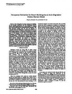
program, the state space must be enlarged to include the positive and negative parts of ri as separate variables. Patterns: In applications over a large region with limited information a utility function that favors certain patterns of behavior might be considered, including clustering and lane formation. Seasons or times of the day: The utility functions may vary seasonally, with time of the day or even days of the weeks and holidays. For example, a park utility function is usually higher during the day than over night. This changes on a 4th of July, when big crowds gather to watch the fireworks. III. E XPERIMENTAL RESULTS In this section we describe occupancy estimation results obtained in experiments in an office building. A. Sensor and sensor layout Figure 3 shows the building floor layout as well as locations of the sensors. Three classes of sensors were used in the experiment: (i) Digital Video Cameras, (ii) Passive Infrared (PIR) Detectors and (iii) CO2 sensors. In order to monitor occupancy flow, 10 video cameras were installed across pre-defined lines located at the 5 entrances of the floor, and in the middle of the hallways. In order to cover the gaps, twelve non-directional PIR sensors were located in pairs between the video cameras. Additionally, 15 CO2 sensors were distributed in different rooms. 1) Video Cameras: Video cameras provide information regarding people count and the direction of the flow. These cameras were found to exhibit significant error in the form of variance and bias, arising from three main factors. Firstly, during early and late hours, when the lighting condition is poor, a single person crossing may be counted multiple times. Secondly, turning a light switch on or off may trigger a sensor count. Lastly, the video system may count several crossings during a time interval in which there are occupants loitering close to the camera. Such events lead to a significant positive bias. 2) PIR Detectors: PIR detectors provide indication of motion within sensor range. The PIR detectors employed in this study were non-directional. By using them in pairs, they were rendered directional. Consequently, the twelve PIR sensors were grouped into six pairs. Preprocessing of

PIR sensor data was performed to eliminate drift in data logging time stamps over the course of days. In addition the directional information was inferred based on the time difference between event time for each pair of detectors. 3) CO2 Sensors: CO2 sensors provide concentration readings in parts per million (ppm), which is indicative of the occupancy. However, reliably correlating CO2 levels with the actual occupancy is difficult due to high variability and the slow response time of the CO2 sensors. This variability arises due to fluctuations in ambient CO2 levels, HVAC system settings and door open/close status. Additionally, CO2 sensors suffer from poor response time (about 10-20 minutes for sensors employed in this study) due to delay between occupancy level increase and build up of CO2 concentration. In next section we show how the bias and variance in the occupancy and flow measurements, can be systematically handled in the SUN framework. B. SUN Implementation The estimation algorithm used in the experiments was a special case of the convex program (5), with the objective function, kφ0

−

φ¯0 k2Σ−1 + 0

T −1 X

Py (φ(t), y(t))

t=0

+


kφ(t + 1) − At φ(t)k2Σ−1 − Ux (φ(t)) (11) d

where, Py and Ux are quadratic functions of φ = (x, r). In addition bound constraints were imposed on occupancy and flow. As a result the convex program, simplifies to a quadratic optimization problem. In our current implementation, the building floor is divided into 11 zones which is dictated by the location of video and PIR sensors (see Figure 3 for zone definition). The matrix At in the dynamics penalty term in the objective (11) is taken to be the identity matrix. Incorporating CO2 measurements in above framework requires additional modifications. This is described in detail below, along with the construction of Py , Ux and the choice of bounds. 1) Penalty function for Video Cameras and PIR Motion Detectors: It was pointed out in section III-A that video sensors suffer from large bias and variance. PIR detectors on the other hand, completely miss on the people count information. Statistical models are required in order to adaptively correct for such errors. For instance, consider PIR sensors and assume that we have a prior probability distribution pij (r), that the flow from zone i to zone j is rij = r, given that the PIR indicates movement. Let {pi : i = 0, 1} be two such prior distributions (see Figure 4 top two panels), where p0 is the probability distribution when the PIR sensor does not indicate any activity and p1 is the distribution when it is activated. Assume that these probabilities are log-concave: pi (r) = e−Pi (r) where, Pi is a linear piecewise utility or soft penalty function, introduced in section II-C.2. By convolving these penalty

Probability Distribution

Sensor Penalty/Utility

beginning and end of the period. The SUN estimator returns estimates {φˆk (t : T ) : t = 0, . . . , T } of occupancy and flow for each day k = 1, . . . , N . Based on these estimates collected over several weeks, we obtained estimates of the mean and variance of occupancy in various zones, for each hour

8

P0(rij)

p0(rij)

1

0.5

6 4 2

0

0

0.5

0

1

0

0.5

r

8

0.6

6

P1(rij)

p1(rij)

ij

0.8

0.4 0.2 0

1

r

ij

4

µi = N −1

2 0

0.5

1

1.5

0

2

k=1 0

0.5

1

r

1.5

2

r

ij

ij

Y

0.5

0

5

10

15

20

25

30

35

40

p

(b xki − µi )2

k=1

45

t

Ux (x) =

0.2

Nz X

Ui (xi ),

i=1

0.1 0 20

N X

σi2 = N −1

x bki ,

where, i = 1, · · · , Nz with Nz = 11 being the total number of zones. This information can be translated to “utility” in the SUN estimator, as

ij

1

0

N X

22

24

26

28

30

32

34

36

38

where,

40

rij

15

Ui (xi ) = − 21 (xi − µi )2 /σi2

P

10 5 22

24

26

28

30

32

34

36

38

40

rij

Fig. 4. When {Pi , i = 0, 1} has a small support (Top two panels), the convolutions preserve the convexity (Bottom Panel, last figure). The convolved utility P can be approximated by a quadratic.

functions, we can obtain the probabilistic model at any time scale desired for occupancy estimation. The convolved function, which we would denote by P , is no longer guaranteed to be convex. However, from numerical experiments we found that, when Pi has small support, the convolutions preserve this convexity, and in fact P can be very well approximated by a quadratic as shown in the bottommost panel in Figure 4. Indeed, if Pi in the convolution were Gaussian probability distributions, the resulting convolution would be Gaussian with mean equal to the sum of the means, and variance equal to the sum of the variances. Motivated by this, we take the sensor penalty term Py in (11) to be of the form

and can be used for on-line estimation. The minus sign comes from the fact that utility is to be maximized. We applied this smoothing procedure on sensor data from 16 days to obtain the mean and variance of occupancy for the different zones. Figure 5 shows hourly occupancy estimate at building level obtained for 4 (among 16) days obtained in this process, and also the mean and variance of occupancy as a function of time for two different zones. Day2

Day1 40 40

30 20

20 10

Occupancy

0 20

0

0

5

10

15

20

0

0

5

10

15

20

40 20

0

20

0

5

10

15

20

0

0

5

t(hrs)

10

t(hrs) σ 10

5

Pyij ,

8

(12)

i=1 j>i

Zone 1

Py (φ, y) =

20

40

µ

Nf X X

15

Day4

Day3

4 6 3 4

2

2

1

where, Nf is the total number of flow sensors (video and PIR) and

5

10

15

20

is a soft penalty for each sensor, with bij being the bias that 2 depends on the measurement yij and σij being the variance. These parameters of soft penalty functions for video count and PIR sensors were obtained by an extensive statistical analysis of the ground truth occupancy flow data. 2) Utility for Occupancy: We used smoothing procedure to obtain occupancy utility functions at zonal level by using historical data of the building usage pattern. In smoothing, at the end of each day, say at 11pm, the algorithm (11) is run over the period [0, T ] = [12am ... 11pm], with the constraint that occupancy is near zero on the boundaries, i.e. at the

10

15

20

5

10

15

20

1

0.8

(13)

5

1

Zone 5

2 Pyij (rij , yij ) = 21 (yij − bij (yij )))2 /σij ,

0

0.8 0.6 0.6 0.4

0.4

0.2 0

0.2 5

10

15

t(hrs)

20

t(hrs)

Fig. 5. Top Two Panels: Hourly occupancy estimate at building level for 4 workdays using the smoothing procedure. Bottom Two Panels: Mean and variance of occupancy as a function of time for 2 of the 11 zones.

3) Incorporating Partial Information from CO2 Sensors: Recall that CO2 sensors were installed only in some rooms and provide additional occupancy information for portions of each zone (see Figure 3). The simplest way to incorporate

where, x(t) is a vector of occupancy levels, at time t, for all zones that do not have CO2 sensor-equipped rooms within each zone, xc (t) is a vector of occupancy levels for rooms with CO2 sensors at time t and r(t) is the vector of flow rates as before. The mass balance constraint for each zone takes the form

500 480 460 440 420 400 380 2

4

6

8

10

2

4

6

8

10

12

14

16

18

20

22

24

12

14

16

18

20

22

24

800

2

Co Concentration (ppm)

such partial information into the existing formulation (11) is to augment the vector of decision variables with the estimated occupancies of rooms equipped with a CO2 sensor. Consequently, the definition of vector occupancy x(t) also gets modified. More precisely, the decision variable φ(t) becomes   x(t) φ(t) =  xc (t)  , (14) r(t)

700 600 500 400

t(hrs) 16 14 12

+

j=1

X j

bi (t) + x bcj (t + 1) = x

rˆji (t) −

X

rˆil (t),

Nci X j=1

x bcj (t)

Occupancy

x bi (t + 1) +

Nci X

8 6 4

l

2

where Nci is the number of rooms equipped with CO2 sensors in ith zone. The mean and variances required for the CO2 utility functions are computed empirically using 16 days of CO2 sensor measurement data, similar to as described in the section III-B.2. However, before extracting the mean and variance for CO2 utility functions, significant preprocessing of CO2 measurements is required. First, in order to eliminate the day to day variations, the CO2 readings of a typical day is subtracted by a day of CO2 data without any occupancy (such as a weekend or a holiday). The top and middle panels in Figure 6 shows CO2 profile in an unoccupied and occupied room, respectively. The CO2 measurements are then denoised using a 4th order low-pass FIR digital filter. The model used to relate the filtered CO2 measurements yi (t) (with background CO2 level subtraction) to the underlying occupancy estimates xci (t) (accounting for a single step 10 minute time lag) is given by yi (t + 1) = αyi (t) + βb xci (t),

10

0 midnight

7am

noon

5pm

midnight

7am

noon

Fig. 6. Top panel shows CO2 concentration with no occupancy, while the middle panel shows a typical profile on a weekday. Bottom panel shows the modeled occupancy (black line) and actual occupancy (red).

12 - 6am 6am - 9am 9am - 12pm 12pm - 1pm 1pm - 5pm 5pm - 6pm 6pm - 9pm 9pm - 12am

Office 1 1 3 2 3 2 2 1

Small CR 0 0 10 5 10 5 0 0

Big CR 0 0 20 10 20 10 0 0

TABLE I O CCUPANCY BOUNDS FOR DIFFERENT TYPES OF ROOMS (CR STANDS FOR CONFERENCE ROOMS ).

(15)

where the coefficients α and β are fitted using the ground truth occupancy data and corresponding CO2 measurement data available, as shown as a red curve in bottom panel in Figure 6. The modeled occupancy is set to zero when the CO2 level is below a “tolerance” of 50ppm; the observed variability in CO2 measurements for zero occupancy is approximately 50ppm. The bottom panel in Figure 6 shows the correspondence between the actual and modeled occupancy using this approach. 4) Bounds on Occupancy and Flow Rates: The lower bound on occupancy level in any zone is set to be zero, while the zone level upper bound is taken to be summation of the upper bounds imposed on each rooms in the zone. For a room, we used the room level upper bounds given in Table I, which depends on the type of room and its expected usage pattern over the course of a day. Currently, the flow

rate bounds are set high enough such that it never constrains the problem. C. Occupancy Estimation Results In this section we compare the SUN estimator with a conventional estimator that relies solely on flow measurements. The accuracy of the two methods is assessed with respect to the ground truth occupancy distribution which was obtained manually by analyzing individual video frames and correcting them for under counts, over counts, and misdetects. In order to obtain building level occupancy ground truth, five peripheral video cameras (labeled as 1,2,3,5, and 9, see Figure 3) which monitor people traffic at entrance and exit locations were chosen. In addition two video people count sensors (7 and 8, see Figure 3) were used in the interior of building to assess the accuracy of occupancy estimates at

70

0

10

−10

−10

−30 8 10 12 14 16 18

6

8 10 12 14 16 18

6

8 10 12 14 16 18

15

8 6 4 2 0

0 10 5 8 10 12 14 16 18

5 0 −5 −10

6

8 10 12 14 16 18

0

10

−10

8 10 12 14 16 18

10

0

20

6

8 10 12 14 16 18

10 0

6

8 10 12 14 16 18

6

8 10 12 14 16 18

6

8 10 12 14 16 18

Noon

5pm

Fig. 9. Occupancy estimation at building level using, conventional people count estimator(black), SUN estimator (blue) and ground truth (red).

0 −10

0

7am

−20

0 6

−20 20

−30 6

8 10 12 14 16 18

t(hrs)

Fig. 7. Zone level occupancy estimates obtained from conventional people count estimator. 10

Occupancy

30 20

−4 6

−10

40

−2

20

5

10

0

0

6 8 10 12 14 16 18

20

6 8 10 12 14 16 18

0

10

5

5

0

0

0

6 8 10 12 14 16 18

10

6 8 10 12 14 16 18

20

20

5

10

10

0

0

6 8 10 12 14 16 18

6 8 10 12 14 16 18

0

6 8 10 12 14 16 18

0

Fig. 10.

Noon

5pm

Similar plot as above but at zonal level.

6 8 10 12 14 16 18

6 8 10 12 14 16 18

6 8 10 12 14 16 18

Fig. 8. Zonal level occupancy estimates obtained from SUN (blue). Also shown in red are the zonal occupancy bounds used during SUN estimation.

the zonal level. This zone was chosen, since it is one of the high traffic areas in the building and shows wide variability in occupancy levels during the course of the day. The estimation error was computed as the average % error, using Tf X 1 |x(t) − x b(t)| , Tf − T0 x(t)

(16)

t=T0

where, x(t) is the ground truth occupancy and, x b(t) is its estimate, with T0 = 6 hrs corresponding to 6am and Tf = 18hrs corresponding to 6pm. The conventional estimator is based on simple counting, X X x bi (t + 1) − x bi (t) = rˆji (t) − rˆil (t), (17) j

5

7am

t(hrs)

E=

10

6 8 10 12 14 16 18

10 0

15

0

5

20

Occupancy at Zone Level

Occupancy

50

−20

0 6

60

0

−20

50

Occupancy

100

l

where, rˆji (t) are the estimates of people count from video cameras. The estimator is initialized to a zero occupancy level at 12am. Figure 7 shows occupancy estimates in the 11 zones based on this estimator over a typical weekday. The occupancy levels are either unexpectedly high at the

end of the workday in many zones (notably among them being the zone 1) or have non physical negative values. The lack of observability is evident from these plots: the sensors providing flow measurements that have a small positive bias that is integrated over the course of the day results in a massive error at 5:00 p.m. At building level (see Figure 9), the occupancy variation is more reasonable due to cancelation of mutual errors, although high occupancy at the end of the day is again unrealistic. The average estimation error based on this simplistic people count estimator is around 70%. Figure 10 shows a similar plot, but at zonal level (this zone is made up of zones 7 and 8, see Figure 3) with an estimation error of 30%. In the SUN implementation we studied in detail the importance of different terms in the objective function (11). Not surprisingly, it was found that the best estimates are obtained by a suitable combination of the different terms, each of which model different source of information: we only report the final results. The zone level SUN estimates are shown in Figure 8, while the blue curve in Figure 9 shows the estimates at the building level. These estimates were obtained for 10 minute intervals by using a backward receding horizon of 1 hour, i.e. T = 60 minutes in objective (11). The quadratic program solver in MATLAB was used for numerical implementation of SUN algorithm. The initial estimates at 12am were taken to be zero both for the occupancy and the flow rate. The estimation error at building level is found to be approximately 11%, while that at zonal level is around 21% (see Figure 10). Inspite of the large bias and variance in the occupancy and flow measurements, the

SUN estimator yields occupancy estimates that are in good agreement with ground truth, especially at the building level. IV. C ONCLUSIONS We introduced the sensor-utility-network (SUN) method to accurately estimate occupancy levels and distribution in buildings. Based on inputs from a variety of distributed sensor measurements (video, PIR, access control, and CO2 ), along with historical data regarding building utilization, the SUN estimator produces occupancy estimates through the solution of a receding-horizon convex optimization problem. In our experiments we found that this approach reduced average occupancy estimation errors at building level from 70% obtained using conventional estimator, to 11%. There are many challenges that remain to be addressed. These include evaluation of performance of SUN estimator for predictive use, adaptive techniques for learning building usage and associated utility functions, sensitivity of the impact of sensor placement and sensor types on occupancy estimation performance. Finally, to make SUN estimator scalable, decentralized algorithms should be developed. V. ACKNOWLEDGEMENTS The funding provided by United Technologies Research Center for this work is greatly appreciated. The authors are grateful to Igor I. Fedchenia (UTRC) for extracting ground truth occupancy data for comparison with the SUN occupancy estimates. The first author would also like to acknowledge a partial support by NSF under grant CCF 0729031. Any opinions, findings, and conclusions or recommendations expressed in this material are those of the authors and do not necessarily reflect the views of the NSF. R EFERENCES [1] H. Chen. Similarity-based analysis for large networks of ultra-low resolution sensors. Technical Report, 2006. [2] Kun Deng, Wei Chen, Prashant G. Mehta, and Sean Meyn. Resource pooling for optimal evacuation of a large building. In 47th IEEE Conference on Decision and Control, Cancun, Mexico, December 911 2008. [3] T. M. Garwin, N. A. Pollard, and R. V. Tuohy, editors. Project Responder: National Technology Plan for Emergency Response to Catastrophic Terrorism. The National Memorial Institute for the Prevention of Terrorism / United States Department of Homeland Security, 2004. [4] G. C. Goodwin, M. M. Seron, and J. A. De Don´a. Constrained control and estimation. An optimisation approach. Communications and Control Engineering. Springer-Verlag, London, 2005. [5] Xiaoshan Pan Kincho Law, Kenneth Dauber. Energy impact of commercial building controls and performance diagnostics: Market characterization, energy impact of building faults and energy savings potential. Technical Report TIAX Reference D0180, TIAX LCC for DOE, November 2005. [6] D. J. C. MacKay. Information Theory, Inference, and Learning Algorithms. Cambridge University Press, 2003. available from http://www.inference.phy.cam.ac.uk/mackay/itila/. [7] S. Meyn, Y. Lin, M. S. Oggianu, A. Surana, and I. Fedchenia. System and method for occupancy estimation and monitoring. USPTO patent application under review, 2008. [8] S. P. Meyn. Control Techniques for Complex Networks. Cambridge University Press, Cambridge, 2007. [9] National Fallen Firefighters Foundation. Report of the National Fire Service Research Agenda Symposium, Emmitsburg, MD, 2005.

[10] J.S. Niedbalski, P. G. Mehta, and S. P. Meyn. Model reduction for reduced order estimation in traffic models. In IEEE American Control conference, Seattle, USA, pages 914–919, June 11-13 2008. [11] M. Schreckenberg and S.D. Sharma, editors. Pedestrian and Evacuation Dynamics. Springer, Berlin, 2002. [12] J. M. Smith and D. Towsley. The use of queuing networks in the evaluation of egress from buildings. Environment and Planning B: Planning and Design, 8(2):125–139, 1981. [13] Robert Tomastik, Satish Narayanan, Andrzej Banaszuk, and Sean Meyn. Model-based Real-Time Estimation of Building Occupancy During Emergency Egress. 4th International Conference on Pedestrian and Evacuation Dynamics. http://www.ped2008.com/, February 27–29 2008. [14] Peng Wang, Peter B. Luh, Shi-Chung Chang, and Jin Sun. Modeling and optimization of crowd guidance in building emergency evacuation. In Proceedings of the 2008 IEEE Conference on Automation Science and Engineering, 2008.