doi:10.1038/nature06067
LETTERS A sequence-based variation map of 8.27 million SNPs in inbred mouse strains Kelly A. Frazer1, Eleazar Eskin2, Hyun Min Kang3, Molly A. Bogue4, David A. Hinds1, Erica J. Beilharz1, Robert V. Gupta1, Julie Montgomery1, Matt M. Morenzoni1, Geoffrey B. Nilsen1, Charit L. Pethiyagoda1, Laura L. Stuve1, Frank M. Johnson5, Mark J. Daly6,7, Claire M. Wade6,7 & David R. Cox1
A dense map of genetic variation in the laboratory mouse genome will provide insights into the evolutionary history of the species1 and lead to an improved understanding of the relationship between inter-strain genotypic and phenotypic differences. Here we resequence the genomes of four wild-derived and eleven classical strains. We identify 8.27 million high-quality single nucleotide polymorphisms (SNPs) densely distributed across the genome, and determine the locations of the high (divergent subspecies ancestry) and low (common subspecies ancestry) SNP-rate intervals2–6 for every pairwise combination of classical strains. Using these data, we generate a genome-wide haplotype map containing 40,898 segments, each with an average of three distinct ancestral haplotypes. For the haplotypes in the classical strains that are unequivocally assigned ancestry, the genetic contributions of the Mus musculus subspecies—M. m. domesticus, M. m. musculus, M. m. castaneus and the hybrid M. m. molossinus—are 68%, 6%, 3% and 10%, respectively; the remaining 13% of haplotypes are of unknown ancestral origin. The considerable regional redundancy of the SNP data will facilitate imputation of the majority of these genotypes in less-densely typed classical inbred strains to provide a complete view of variation in additional strains. Classical strains are derived from a limited number of founding mice that were genetically diverse owing to the mixture of subspecies of the genus Mus2,3: M. m. musculus, M. m. castaneus, M. m. domesticus and the hybrid M. m. molossinus (Fig. 1). In contrast, most of the wildderived strains used in research are largely genetically pure because they are derived from mice captured in the wild, which were inbred to homozygosity4,5. The unique breeding history of classical strains is reflected in their genomic structure; recent pairwise sequence comparisons reveal alternating intervals of low and high sequencevariation, representing segments of the genome where the two strains have either common (for example, both domesticus) or divergent (for example, one domesticus and one musculus) subspecies ancestry, respectively6–10. The locations and boundaries of the genomic intervals composed of common and divergent ancestry sequences are different for each pair of classical strains and need to be empirically determined. Resequencing methods determine the DNA sequences of individual members of a species for which a high-quality reference genome is available more efficiently than de novo sequencing. Here, we resequenced the genomes of the 15 mouse strains (Box 1), using oligonucleotide arrays6 designed to query , 1.49 billion bases (58%) of the 2.57-billion-basepair C57BL/6J reference genome11 (NCBI
Build 36) for all possible single-base substitutions12 (Supplementary Fig. 1). These 1.49 billion bases represent primarily unique sequences, but also include some lightly masked repetitive sequence (Supplementary Table 1). Nucleotide variation from the C57BL/6J reference sequence was identified by hybridizing labelled amplified DNA from the 15 strains to the arrays. The arrays were then scanned and the feature intensity data analysed with pattern recognition basecalling and SNP-calling algorithms13,14. To make the resequencing data available to individual researchers we developed a method for representing the array data as sequence traces analogous to conventional dideoxy sequencing (Supplementary Fig. 2). We identified 8,266,653 SNPs with unique positions in the mouse genome (NCBI Build 36), the vast majority of which are novel. Of the SNP submissions clustered in dbSNP Build 126, 92.5% were either the only instance of the associated cluster or the member of the cluster submitted first. We assessed the quality of our SNP data, determining that the false-positive rate of discovery is 2% and the accuracy of our genotype calls is greater than 99% (Supplementary Information). To assess our false-negative rate for SNP discovery we selected all SNPs on chromosome 4 where the A/J strain in the Celera WGS resequencing data15 had a different allele from the C57BL/6J sequence and for which the same genotypes were validated by an independent study at the Broad Institute (unpublished data). This resulted in a set of 5,553 validated SNPs on chromosome 4, of which 3,936 SNPs (70.9%) were in sequences tiled on the arrays and 2,366 (42.6%) had the alternate allele detected in at least one of the 15 strains analysed by array-based resequencing. From this analysis we estimate that 2,366 out of 3,939, or ,60%, of SNPs in tiled sequences and ,43% of all SNPs present in the classical strains were identified in our array-based resequencing study. Of the 8.27 million SNPs identified among all strains, 3.39 million (41%) were polymorphic when only the 11 classical strains were considered and 6.46 million (78%) were polymorphic when only the 4 wild-derived strains were considered. Given that we discovered 3.4 million SNPs in the 12 classical strains and have a 43% SNP discovery rate, we estimate that in total there are ,8 million SNPs in the classical strains. Interestingly, 1.81 million (22%) of the SNPs polymorphic among the classical strains were monomorphic in the wild-derived strains, indicating that a substantial amount of un-sampled ancestral genotypes contributed to the generation of the classical strains. With a total of 2.57 billion base pairs of available mouse genome reference sequence, the 8.27 million SNPs identified among all strains yields an average density of 1 SNP per 311 base pairs (Supplementary
1
Perlegen Sciences, 2021 Stierlin Court, Mountain View, California 94043, USA. 2Department of Computer Science and Department of Human Genetics, University of California, Los Angeles, Los Angeles, California 90095, USA. 3Department of Computer Science and Engineering, University of California, San Diego, La Jolla, California 92093, USA. 4The Jackson Laboratory, Bar Harbor, Maine 04609, USA. 5Toxicology Operations Branch, National Institute of Environmental Health Sciences, Research Triangle Park, North Carolina 27709, USA. 6 Broad Institute of Harvard and MIT, 7 Cambridge Center, Cambridge, Massachusetts 02142, USA. 7Center for Human Genetic Research, Massachussets General Hospital, 185 Cambridge St, Boston, Massachusetts 02114, USA.
1 ©2007 Nature Publishing Group
LETTERS
NATURE
Ancestral musculus subspecies
a
b
c
d
musculus Eastern Europe Russia Northern China
East Asian ‘fancy’ mouse
molossinus Japan
European ‘fancy’mouse
castaneus
Classical inbred mouse strains domesticus (WSB/EiJ) 68% molossinus (MOLF/EiJ) 10% musculus (PWD/PhJ) 6% castaneus (CAST/EiJ) 3% Unknown origin 13%
Western Asia Southeastern Asia Southern China
domesticus Western Europe
Approximate timeline
e
~1,000,000
~10,000
~1,000
~100
(Years)
Figure 1 | Origin of modern classical strains. a, The subspecies musculus, castaneus and domesticus subspecies diverged from a common ancestor about one million years ago. b, The subspecies molossinus is a more recent hybrid between musculus and castaneus16. c, In the eighteenth century, mouse fanciers in Japan and China inter-bred the Asian Mus musculus subspecies to produce varieties of mice with different coat colours and
behavioural characteristics as pets2,16. d, In Victorian England, ‘fancy’ mice were imported from Asia and bred with local mice. In the early twentieth century, mating programmes using a limited number of founding ‘fancy’ mice were started in the USA, giving rise to many of the modern classical strains2. e, The relative contributions of the Mus musculus subspecies to haplotypes in classical strains.
Table 2); for the subset of SNPs polymorphic only in the wild-derived strains, the density is 1 SNP every 397 base pairs; and for the subset of SNPs polymorphic only among the classical strains, 1 SNP every 756 base pairs. Given our 43% SNP discovery rate, these data agree with previous estimates of classical strain diversity of 1 SNP every 250–300 base pairs7. To investigate the uniformity of genome coverage of our SNP set, we examined the distribution of inter-SNP distances. For the complete SNP set, 95% of the inter-SNP intervals are 1 kb or less, and 99.7% are 10 kb or shorter (Supplementary Fig. 3a). Considering the wild-derived strains and the classical strains separately, the equivalent values are 93% and 99.5% for wild-derived strains, and 87% and 98.7% for classical strains. Thus, the vast majority of inter-SNP distances are shorter than 1 kb. We also examined the fraction of the available genome within a given maximum distance of a typed SNP (Supplementary Fig. 3b). For our complete SNP set, 75% of the genome was within 1 kb of an SNP, and 93% of the genome was within 5 kb of an SNP. For SNPs polymorphic in the wild-derived inbred strains, 70% and 91% of the genome was within 1 kb and 5 kb of an SNP, respectively. For SNPs polymorphic in the classical strains,
53% and 81% of the genome was within 1 kb and 5 kb of an SNP, respectively. The inter-SNP interval and maximum distance analyses provide complementary information, with both indicating that the genome coverage of our 8.27 million SNP set is dense and uniform. We next determined the common (low SNP-rate) and divergent (high SNP-rate) ancestral intervals across the genome for each pairwise combination of the classical strains, using a dynamic programing algorithm to identify regions of shared ancestry among the strains. We included the genotypes of the reference strain C57BL/ 6J so in total there were 12 strains analysed. For the 66 pairwise comparisons, there was an average of 5,519 low SNP-rate (1 SNP per 21 kb) and/or high SNP-rate (1 SNP per 440 base pairs) intervals across the genome (Supplementary Table 3). The low SNP-rate intervals contained 62% of the bases and extended for an average of 568 kb, whereas the high SNP-rate intervals contained fewer bases (38%) and were shorter, at 355 kb. To generate a haplotype map across the genome, we mapped all the ancestry breakpoints in the 12 classical strains, defined as locations at which any of the pairwise comparisons transited from a low SNP-rate to a high SNP-rate interval or vice versa. The regions between these breakpoints represent segments in which all strains have a single unbroken ancestral haplotype (Fig. 2) Our genome-wide map consists of 40,898 segments with an average length of 58 kb (ranging from 1 kb to 3 Mb), covering approximately 90% of the mouse genome (Supplementary Table 4). On average there are 3.05 6 0.98 different haplotypes observed per segment in the 12 classical strains. In each pairwise comparison the low SNP-rate intervals extend through approximately 10 segment boundaries. To characterize the total amount of genetic variation in a region of a given size, we consider strain distribution patterns (SDPs) or distinct groupings of the strains that are based on SNPs within a region (Supplementary Table 5). The number of SDPs represents the number of nonredundant SNPs within a defined region (that is, the number of SNPs required to capture the variation content of that region). Less than 2% of the SNPs in a 50-kb region represent singleton SDPs (and less than 0.5% of the SNPs in a 5-Mb window). The number of SDPs accounting for 95% of all patterns observed is 3.3 in 50-kb windows and only 28.4 in 5-Mb windows. Thus, although slightly fewer than half of all SNPs in the classical strains were discovered, the redundancy demonstrated in the SDP analysis indicates that very few distinct variation patterns are uncaptured by this data set. The inclusion of four wild-derived strains in our study allowed us to determine the ancestry of many of the haplotypes in the classical
Box 1j | Fifteen mouse strains selected for resequencing The following criteria were considered in the selection process: widespread use in research; availability of ancillary genetic resources such as recombinant inbred and/or consomic lines18; inclusion in the Mouse Phenome Project19–21; maximization of phenotypic and genetic diversity; and ease of breeding to enable follow-up studies. The 15 selected strains can be divided into three groups: $ Group one consists of eight classical strains commonly used for research, of which several have served as progenitors of recombinant inbred strains and/or are part of consomic panels with C57BL/6J (www.jax.org/); these are: 129S1/SvImJ, A/J, AKR/J, BALB/cByJ, C3H/HeJ, DBA/2J, FVB/NJ, NOD/LtJ. $ Group two consists of three classical strains that are useful models of complex human diseases: BTBR T1tf/J, which is used as a model to study behavioural abnormalities22 and autism23; KK/HlJ, which was chosen because of its distinct lineage from the other strains in the study1 and its use as a model for type II diabetes24, and NZW/ LacJ, which is used as a model to study autoimmune diseases. $ Group three consists of four wild-derived strains: CAST/EiJ (castaneus), MOLF/EiJ (molossinus), PWD/PhJ (musculus) and WSB/ EiJ (domesticus). Because the origins of the classical strains stem from the interbreeding of the Mus musculus subspecies (Fig. 1), this group provides important information on ancestral sequence diversity. 2
©2007 Nature Publishing Group
LETTERS
NATURE
C57BL/6J DBA/2J A/J BALB/cByJ C3H/HeJ AKR/J FVB/NJ 129S1/SvlmJ NOD/LtJ BTBR T+ tf/J NZW/LacJ KK/HIJ Chromosome 04 30.0 positions (Mb)
31.0
32.0
33.0
34.0
35.0
36.0
37.0
38.0
39.0
40.0
41.0
42.0
43.0
44.0
45.0
46.0
47.0
48.0
Figure 2 | Ancestral haplotype map for an 18-Mb region on chromosome 4. Colours represent an ancestral origin of WSB/EiJ (yellow), PWD/PhJ (red), CAST/EiJ (green) or MOLF/EiJ (blue) strains. For the 12 classical inbred
strains, each segment is coloured to indicate its predicted ancestral origin. The grey colour represents gaps in the SNP coverage and the black colour represents either ambiguous or unknown ancestral origin.
strains. A dynamic programming algorithm assigned the most-likely wild-derived ancestor for each classical strain in each segment and mapped these predictions to the ancestry breakpoints. On average, ancestry for 67% of the genome of each classical strain could be unequivocally assigned to one of the Mus subspecies. Ancestry for 10% of the genome was unequivocally different from all four wildderived strains. The remaining portion of the genome has ambiguous ancestry because either the region matched two or more of the wildderived strains (3%) or there was insufficient coverage to determine ancestry (20%) because the algorithm required all 4 wild-derived strains to be successfully genotyped. For the classical strain haplotypes that could be assigned ancestry, the domesticus strain (WSB/EiJ) matched 68%, the molossinus strain (MOLF/EiJ) 10%, the musculus strain (PWD/PhJ) 6%, and castaneus (CAST/EiJ) 3%, with the remaining 13% unequivocally ancestrally divergent from the four wild-derived strains (Fig. 1, Supplementary Table 6). Therefore, of the Mus subspecies, domesticus made the largest genetic contribution to the classical strains, a finding consistent with previous reports that were based on candidate region analyses7,16. Applying a similar analysis to the hybrid molossinus strain we identify its ancestry as 57% musculus, 12% castaneus, 7% domesticus and 24% of unknown ancestry, which is also consistent with previous reports. Interestingly, the ancestral contribution represented by each of the four wild-derived strains greatly differs across the genome even at the level of entire chromosomes (Table 1). In the regions with unambiguous ancestry, domesticus contribution ranges from 80%
on chromosome 18 to only 51% on chromosome 14. The equivalent range for molossinus is from 22% on chromosome 4 to only 1% on chromosome 16, for musculus from 28% on chromosome 14 to only 1% on chromosome 5, and for castaneus from 8% on the chromosome 19 to less than 1% on chromosome 18. Although the relative ancestral contributions of the 4 wild-derived strains to each of the 12 classical strains is highly similar at the genome-wide level, the distribution of ancestral origins varies greatly at the chromosome level (Supplementary Table 7). For example, the molossinus contribution on chromosome 7 is 2% in C57BL/6J and 19% in DBA/2J, whereas on chromosome 12 the molossinus contribution is 14% in C57BL/6J and 1% in DBA/2J. Our data are accessible through NCBI databases, with SNPs deposited in dbSNP and trace files in the Trace Archive. In addition, we have established a website (http://mouse.perlegen.com), which researchers can use to download SNPs, genotypes and LR-PCR primer pairs, all of which are currently mapped to NCBI Build 36. The site hosts a genome browser17 (Supplementary Fig. 4)—which allows users to visualize, for specific genomic intervals, the locations of SNPs, LR-PCR primer pairs, and intervals of non-repetitive sequence that were assayed in this study—and a webserver, where researchers can browse and download the ancestral haplotype map to obtain ancestry information for any region of the mouse genome. We anticipate that data generated from SNP sets that are less dense but genotyped in strains not included in our study, such as the Broad Institute resource of 150,000 genome-wide genotypes on the most commonly used 100 classical strains, will be used to map additional strains to our ancestral haplotype map. This will allow genotypes for most of our 8.27 million SNPs to be imputed for these unsequenced strains on the basis of their shared ancestral haplotypes.
Table 1 | Ancestral contribution of each of the four wild-derived strains and an unknown strain, which is unequivocally ancestrally divergent from any of the four wild-derived strains, for each chromosome Chromosome
WSB/EiJ
PWD/PhJ
CAST/EiJ
MOLF/EiJ
Unknown
01 02 03 04 05 06 07 08 09 10 11 12 13 14 15 16 17 18 19 X Genome-wide
0.6684 0.6337 0.7054 0.6066 0.6296 0.6384 0.7348 0.7166 0.5613 0.6799 0.6907 0.7193 0.7113 0.5107 0.7166 0.7916 0.6725 0.7999 0.7537 0.8712 0.6846
0.0818 0.0267 0.0261 0.0554 0.0082 0.0787 0.0309 0.0373 0.1763 0.0260 0.0196 0.0200 0.0688 0.2805 0.0465 0.0095 0.0494 0.0218 0.0105 0.0179 0.0562
0.0202 0.0542 0.0463 0.0136 0.0122 0.0286 0.0103 0.0061 0.0288 0.0160 0.0158 0.0677 0.0143 0.0099 0.0403 0.0347 0.0543 0.0033 0.0776 0.0811 0.0304
0.0930 0.1935 0.0763 0.2227 0.2215 0.1005 0.0761 0.0756 0.0996 0.1023 0.1749 0.0415 0.0887 0.0985 0.0720 0.0148 0.0348 0.0273 0.0525 0.0145 0.1002
0.1367 0.0919 0.1458 0.1018 0.1286 0.1538 0.1479 0.1644 0.1340 0.1758 0.0990 0.1516 0.1169 0.1005 0.1246 0.1495 0.1890 0.1478 0.1057 0.0154 0.1287
METHODS SUMMARY Array design. The 1.49 million bases tiled on the arrays included at least a portion of 27,915 (97%) of the 28,874 annotated genes in the mouse genome (NCBI Build 36.1), and at least a portion of 201,195 (98%) of the 206,338 annotated exons. To confirm the identity of the strains processed in each hybridization experiment, on all arrays we included a set of 96 SNPs distributed across 8 different genome regions, the genotypes of which allowed unambiguous discrimination between the 15 inbred strains (Supplementary Table 8). Samples. Resequencing was performed using DNA isolated from pedigreed breeding stock animals (Jackson Laboratory Æhttp://www.jax.org/æ). To prepare the DNA samples for analysis, we designed 241,806 long-range PCR (LR-PCR) primer pairs to generate amplicons ranging from 3 to 12 kb in length. Together these primer pairs were used to amplify essentially the entire genomes of each of the 15 strains. Resequencing. High-density oligonucleotide array technology was used as described13,14. Nucleotide variation from the C57BL/6J reference sequence was identified by hybridizing labelled amplified DNA from the 15 strains to the arrays, which were then scanned and the feature intensity data analysed with pattern recognition base-calling and SNP-calling algorithms13,14. 3
©2007 Nature Publishing Group
LETTERS
NATURE
Ancestral haplotype map. To partition the genomes into segments in our pairwise comparisons of the 12 classical strains, we constructed a hidden Markov model with two states for each SNP position (one for high and one for low SNPrate) and applied the Viterbi algorithm to assign each SNP to one of the two segment types. We constructed the haplotype map by defining a block boundary at each position where a segment transited from a low SNP-rate to a high SNPrate segment or vice versa in one of the 66 pairwise comparisons. To identify ancestral origins of haplotypes, we constructed a hidden Markov model with five states for every SNP, with four states each representing one of the four wildderived strains and one state representing an unknown ancestral origin, and applied the forward–backward algorithm to assign the ancestry to each SNP in each of the classical strains. Full Methods and any associated references are available in the online version of the paper at www.nature.com/nature. Received 14 April 2007; accepted 5 July 2007. Published online 29 July 2007. 1. 2. 3.
4. 5. 6.
7. 8. 9.
10.
11. 12. 13. 14.
Beck, J. A. et al. Genealogies of mouse inbred strains. Nature Genet. 24, 23–25 (2000). Wade, C. M. & Daly, M. J. Genetic variation in laboratory mice. Nature Genet. 37, 1175–1180 (2005). Bonhomme, F., Gue´net, J.-L., Dod, B., Moriwaki, K. & Bulfield, G. The polyphyletic origin of laboratory inbred mice and their rate of evolution. Biol. J. Linnean Soc. 30, 51–58 (1987). Petkov, P. M. et al. An efficient SNP system for mouse genome scanning and elucidating strain relationships. Genome Res. 14, 1806–1811 (2004). Ideraabdullah, F. Y. et al. Genetic and haplotype diversity among wild-derived mouse inbred strains. Genome Res. 14, 1880–1887 (2004). Frazer, K. A. et al. Segmental phylogenetic relationships of inbred mouse strains revealed by fine-scale analysis of sequence variation across 4.6 Mb of mouse genome. Genome Res. 14, 1493–1500 (2004). Wade, C. M. et al. The mosaic structure of variation in the laboratory mouse genome. Nature 420, 574–578 (2002). Wiltshire, T. et al. Genome-wide single-nucleotide polymorphism analysis defines haplotype patterns in mouse. Proc. Natl Acad. Sci. USA 100, 3380–3385 (2003). Yalcin, B. et al. Unexpected complexity in the haplotypes of commonly used inbred strains of laboratory mice. Proc. Natl Acad. Sci. USA 101, 9734–9739 (2004). Zhang, J. et al. A high-resolution multistrain haplotype analysis of laboratory mouse genome reveals three distinctive genetic variation patterns. Genome Res. 15, 241–249 (2005). Waterston, R. H. et al. Initial sequencing and comparative analysis of the mouse genome. Nature 420, 520–562 (2002). Chee, M. et al. Accessing genetic information with high-density DNA arrays. Science 274, 610–614 (1996). Hinds, D. A. et al. Whole-genome patterns of common DNA variation in three human populations. Science 307, 1072–1079 (2005). Patil, N. et al. Blocks of limited haplotype diversity revealed by high-resolution scanning of human chromosome 21. Science 294, 1719–1723 (2001).
15. Mural, R. J. et al. A comparison of whole-genome shotgun-derived mouse chromosome 16 and the human genome. Science 296, 1661–1671 (2002). 16. Silver, L. M. Mouse Genetics: Concepts and Applications (Oxford University Press, New York, 1995). 17. Stein, L. D. et al. The generic genome browser: a building block for a model organism system database. Genome Res. 12, 1599–1610 (2002). 18. Singer, J. B. et al. Genetic dissection of complex traits with chromosome substitution strains of mice. Science 304, 445–448 (2004). 19. Grubb, S. C., Churchill, G. A. & Bogue, M. A. A collaborative database of inbred mouse strain characteristics. Bioinformatics 20, 2857–2859 (2004). 20. Bogue, M. A. & Grubb, S. C. The Mouse Phenome Project. Genetica 122, 71–74 (2004). 21. Bogue, M. Mouse Phenome Project: understanding human biology through mouse genetics and genomics. J. Appl. Physiol. 95, 1335–1337 (2003). 22. Wahlsten, D., Metten, P. & Crabbe, J. C. Survey of 21 inbred mouse strains in two laboratories reveals that BTBR T/1 tf/tf has severely reduced hippocampal commissure and absent corpus callosum. Brain Res. 971, 47–54 (2003). 23. Moy, S. S. et al. Mouse behavioral tasks relevant to autism: phenotypes of 10 inbred strains. Behav. Brain Res. 176, 4–20 (2007). 24. Nakamura, M. A diabetic strain of the mouse. Proc. Jap. Acad. 38, 348–352 (1962). 25. Ewing, B. & Green, P. Base-calling of automated sequencer traces using Phred. II. Error probabilities. Genome Res. 8, 186–194 (1998). 26. Viterbi, A. J. Error bounds for convolutional codes and an asymptotically optimal decoding algorithm. IEEE Trans. Information Theory 13, 260–269 (1967).
Supplementary Information is linked to the online version of the paper at www.nature.com/nature. Acknowledgements Work was supported by funding from the NIEHS. H.M.K. and E.E. are partially supported by the NSF. H.M.K. is partially supported by a Samsung Scholarship. E.E. is partially supported by the NIH. At Perlegen Sciences, we thank A. Kloek for assistance with manuscript preparation; B. Nguyen, X. Chen, P. Chu, R. Patel, P.-E. Jiao, R. Irikat and J. Kwon for assistance with DNA sample preparation and hybridization of the high-density oligonucleotide arrays; R, Vergara for primer handling; H. Huang and W. Barrett for designing the high-density arrays; T. Genschoreck and J. Sheehan for data quality control; and S. Osborn for assistance with website development and data delivery. At NIEHS, we thank D. A. Schwartz, K. Olden, S. Wilson, L. Birnbaumer, J. Bucher, W. T. Schrader and D. M. Klotz for constructive scientific discussions, and J. A. Lewis and T. Hardee for administrative support. At The Jackson Laboratory, we thank S. Deveau and JAX DNA Resources for DNA sample preparation. Author Contributions L.L.S., J.M., C.L.P. and K.A.F. supervised the experiments. K.A.F., D.R.C., M.J.D., F.M.J., E.J.B. and M.A.B designed the study. H.M.K., E.E, C.M.W., D.A.H., G.B.N., R.V.G. and M.M.M. performed data analysis. K.A.F., with help from E.J.B., D.A.H., E.E. and C.M.W., wrote the manuscript. Author Information Reprints and permissions information is available at www.nature.com/reprints. The authors declare competing financial interests; details accompany the full-text HTML version of the paper at www.nature.com/ nature. Correspondence and requests for materials should be addressed to K.A.F. (
[email protected]).
4 ©2007 Nature Publishing Group
doi:10.1038/nature06067
METHODS High-density oligonucleotide array design. Our study was initiated before the C57BL/6J finished reference sequence was available for the entire mouse genome. Thus, multiple NCBI genome assemblies were used for the design of resequencing arrays for different parts of the genome: Build 33 for chromosomes 2, 4, 11 and X; Build 34 for finished sequences greater than 315 kb from chromosomes 1, 3, 5–10 and 12–19; Build 35 for finished sequences greater than 315 kb from chromosomes 1, 3, 5–10 and 12–19 that were not already covered; and Build 36 for remaining sequence, including chromosome Y and contigs not on the main assembly. The C57BL/6J reference sequence was screened and annotated for interspersed repeats and low-complexity DNA sequences by RepeatMasker using the 2s sensitive setting and the 2m flag to specify murine sequence. Additionally, the sequence was processed using the Tandem Repeat Finder program, masking out repeats with a period of 12 or less. The masked sequence was downloaded from the UCSC Genome Bioinformatics website (http://genome.ucsc.edu/). Of the 2,567,283,971 bases from Build 36, approximately 42.3% are masked as repetitive. Although we primarily tiled the unique non-masked sequences for a fraction of the genome, we used the ‘2div 10’ option in Repeat Masker (http:// www.repeatmasker.org/), which only masks sequences less than 10% diverged from the canonical repeats in the database. For 14,806 intervals distributed across the 19 autosomes, an additional 130,236,585 bp of lightly masked sequence using the ‘–div 10’ option and 10,633,723 bp of unmasked sequence (an aggregate total of 140,900,308 bp resulting from different masking options) were tiled on the arrays (Supplementary Table 1). A total of 1,488,604,099 bp of unique or lightly masked repetitive sequence was used to design high-density oligonucleotide arrays. The arrays were designed such that each of the 1,488,604,099 nucleotides was interrogated by eight 25-mer oligonucleotides (features) that were synthesized and attached to a glass surface (Supplementary Fig. 1). Each set of eight features consisted of four identical to the forward-strand reference sequence from position 212 to 112 with respect to the base to be queried (position 0), with position 0 represented by each of the four bases A, C, G and T. The remaining four features were similarly designed for the reverse strand. The arrays were synthesized by Affymetrix using light-directed photolithography in conjunction with chemical coupling to direct the synthesis of the 25-mer oligonucleotides. For this study, we used large arrays containing approximately 180 million 7 mm features each. With each array able to assay around 22 Mb of unique genomic sequence, we used 68 array designs to cover the entire mouse genome, excluding repetitive sequences. Sample preparation. Using the C57BL/6J reference sequence and the Oligo 6 program we designed 241,806 LR-PCR primer pairs with amplicons ranging from 3 to 12 kb in length, with an average size of 10,336 bp. The primers were typically between 28 and 32 nucleotides in length with a melting temperature of .65 uC. Resequencing was performed using DNA samples isolated from between four and fourteen individual male mice per strain (Supplementary Table 9). PCR reactions (1-plex or 2-plex) were performed as follows (per reaction): 30 ng of genomic DNA from one of the 15 inbred mouse strains was amplified using 1.7 mM of each LR-PCR primer, 0.6 U MasterAmp extra long Taq polymerase (Epicentre Technologies), 20 ng ml21 TaqStart antibody (Clontech), 0.13 TaqStart Antibody buffer (Clontech), 0.4 mM dNTPs, 23 mM Tricine, 3% DMSO, 45 mM Trizma, 2.7 mM MgCl2, 12.6 mM (NH4)2SO4, 2.6 mM KCl and 0.43 MasterAmp PCR Enhancer with Betaine (Epicentre Technologies), in a volume of 12 ml. The reactions were performed using a Perkin-Elmer 9700 thermocycler as follows: initial denaturation for 3 min at 95 uC; 10 cycles at 94 uC for 2 s and 64 uC for 15 min; 28 cycles of 94 uC for 2 s and 64 uC for 15 min, with a 20 s increase per cycle; and a final extension of 60 min at 62 uC. Amplicons to be hybridized together on the array (,11–14 Mb) were combined into one tube, purified using Centricon Plus-20 filter devices (Millipore), quantified using optical density spectrophotometry, and normalized to a concentration of 2 mg ml21. The amplicons were then fragmented to a peak fragment size of 100 bp by incubation of 200 ug of purified PCR product for 30 min at 37 uC in 13 One-Phor-All Buffer PLUS (Amersham) and 0.001 U ml21 amplification grade DNase 1 (Invitrogen). The DNase I was then heat-inactivated at 99 uC for 10 min. The fragmentation reactions were then labelled with either biotin or fluorescein for 90 min at 37 uC in 13 One-Phor-All Buffer PLUS, 13600 U recombinant TdT (Roche Applied Science), and either 0.1 mM each of biotin16-ddUTP and biotin-16-dUTP (Roche Applied Science) or 0.1 mM each of fluorescein-12-ddUPT and fluorescein-12-dUTP (PerkinElmer). A subset of the samples (for 2 out of 68 arrays) were labelled using the same protocol with either biotin as described above or 0.1 mM each of digoxigenin-11-ddUTP and digoxigenin-11-dUTP (Roche Applied Science). Array hybridization. The arrays each containing ,22 Mb of tiled DNA sequence were physically segmented into three chambers and each chamber
was hybridized with a different DNA/hybridization mixture containing labelled target DNA at ,11–14 Mb complexity. The labelled target DNA was prepared for hybridization by combining biotin-labelled amplicons from one strain and fluorescein- or digoxygenin-labelled amplicons from another strain, and adding 40 ml of 10 mg ml21 yeast RNA (Applied Biosystems) and 200 ml 10 mg ml21 herring sperm DNA (Promega), for a total of 640 ml. Combining the DNA from the two different strains labelled with distinct fluorophores in a single array hybridization allowed us to use half the number of arrays otherwise needed (8 copies of each of the 68 individual arrays spanning the genome versus 15 copies of each of these arrays). The 640 ml labelled target DNA was denatured for 10 min at between 90 uC and 100 uC and then snap cooled at 4 uC. It was then added to 4.25 ml of hybridization buffer plus 125 ml 20 mg ml21 BSA, to give a final solution of: 0.08 mg ml21 yeast RNA, 0. mg ml21 herring sperm DNA, 0.5 mg ml21 BSA, 2.94 M TMACL, 0.01 M Tris (pH 8.0), 0.01% Triton X-100, 0.05 nM b-948 biotin control oligo (Sigma-Aldrich), and 0.05 nM fl-948 fluorescein control oligo (Sigma-Aldrich). Hybridization of the target DNA to the microarrays took place at 50 uC for 17 h with constant rotation. After hybridization, the arrays were rinsed with 13 MES and stained for detection of the biotin- and fluorescein-labelled hybridized targets by 30 min incubations at room temperature with the following series of 5 stain solutions (each of which was in 13 MES, 0.1% Triton X-100, and 2.5 mg ml21 BSA): Stain 1 with 5 mg ml21 streptavidin (Invitrogen) plus 10 mg ml21 Alexa 488-rabbit anti-fluorescein antibody (Invitrogen); Stain 2 with 1.25 mg ml21 biotinylated anti-streptavidin (Vector Laboratories); and Stain 3 with 1 mg ml21 streptavidin–phycoerythrin–Cy5 (BD Biosciences) plus 10 mg ml21 Alexa 488 goat antirabbit antibody (Invitrogen). To enhance the flourescein signal, the arrays were then incubated with Stain 4, containing 10 mg ml21 Alexa 488-rabbit anti-fluorescein antibody, and Stain 5, with 10 mg ml21 Alexa 488 goat antirabbit antibody, each for 30 min. The arrays were rinsed with 13 MES between stain incubations, and washed at high stringency in 0.23 SSPE, 0.01% TX-100 for 60 min at 37 uC after the completion of staining. The arrays were then scanned using custom-built confocal scanners. For the arrays using the biotin and digoxygenin labelling strategy, the labelled targets were detected by 20 min incubations at room temperature using the following series of 4 stain reagents (in 13 MES, 0.1% Triton X-100, and 2.5 mg ml21 BSA): Stain 1 with 2.5 mg ml21 Anti-Digoxigenin Ab, clone 1.71.256, mouse IgG1 (Roche Applied Science) plus 5 mg ml21 streptavidin (Invitrogen); Stain 2 with 5 mg ml21 anti-streptavidin (Rabbit) Biotin Conjugated (Rockland Immunochemicals); Stain 3 with 5 mg ml21 Alexa Fluor 647–R-phycoerythrin goat anti-mouse IgG (Invitrogen) plus 1 mg ml21 streptavidin, Alexa Fluor 488 conjugate; and Stain 4 with 9 mg ml21 AffiniPure Mouse Anti-Goat IgG (H1L). To enhance the digoxygenin signal, the arrays were then incubated further with Stain 3 followed by Stain 4. The arrays were rinsed with 13 MES between incubations, and washed at high stringency in 0.23 SSPE, 0.01% TX-100 for 60 min at 37 uC after the completion of staining. The arrays were then scanned using custom-built confocal scanners. Base-calling algorithm. Fluorescence intensity data from an oligonucleotide array scan were first processed to determine an average intensity for each feature on the array. This yielded 8 data points per sequence position: one each for A, C, G and T, for forward and reverse strands. We determined a direct sequence for each strand, consisting of the brightest base at each position (Supplementary Fig. 1). At each position, we also determined the local ‘conformance’ of the array data, as the fraction of base calls that match the reference sequence within a sliding window. For a position where the direct call matches the reference base, this window consists of bases at positions 210 to 110. In the immediate vicinity of an alternative base call, hybridization intensities are reduced owing to the presence of a one-base mismatch base between the target and probe DNA. To avoid the reduced-intensity interval in these cases, we alter the window to span bases 220 to 210, and 110 to 120. A strict base call is made for a sequence position when the ratio of the brightest to next-brightest feature is greater than a threshold of 1.3 for biotin-labelled DNA and 1.1 for fluorescein-labelled DNA, and the conformance around that position is at least 0.80 on both strands. A relaxed base call is made if these criteria are met for just one strand and the other strand is ambiguous (that is, it did not pass either the intensity ratio or conformance requirements). For alternate base calls that do not match the reference sequence, we also require that there are no brighter alternate calls meeting these criteria within positions 25 to 15. SNP detection algorithm. For polymorphism detection, we created a consensus sequence of strict base calls that are confirmed on both strands. Again, alternate consensus calls are excluded if there is a brighter (average intensity over both strands) alternate consensus call within positions 25 to 15. Putative polymorphic sites must also pass a final ‘footprint test’. In this test, normalized intensities for probes matching the reference sequence across positions 25 to 15 were separately averaged for scans that resulted in reference base calls and
©2007 Nature Publishing Group
doi:10.1038/nature06067
alternate base calls. The normalization step adjusts for systematic differences in brightness between scans. An SNP is rejected if the ratio of mean normalized intensity around reference calls to mean normalized intensity around alternate calls is less than 1.5. The footprint test requires a cumulative analysis of a complete set of arrays of the same design. We required at least one consensus reference call and one alternate call to define a polymorphism; positions with no reference calls were rejected. Once a site is determined to be polymorphic, we used relaxed base calls in other samples to determine if they match the reference or alternate bases. This strategy allows us to maintain a low false-positive rate for SNP detection, while maximizing the amount of usable genotype data obtained for each position identified as a likely polymorphism. Trace files. Each trace file represents data for one contiguous fragment of tiled sequence in one orientation. Unlike a conventional sequencing trace, there is a one-to-one correspondence between the trace amplitudes and sequence positions. Data for the reverse tiling were reverse complemented before the trace files were generated, so that the forward and reverse reads were both reported for the forward strand of the reference sequence. The trace files contain all the experimental information required to apply our SNP discovery algorithm. However, owing to round-off of the intensity data in the traces, there may be minor differences in results obtained from the trace files compared with using the raw data. Each trace also carries descriptive information. Supplementary Table 10 explains how to interpret these descriptive fields for Perlegen resequencing traces, and can be used to supplement the NCBI Trace Archive documentation. Using this information, a user can group together all traces from the same scanned image, and all scans from a single hybridization experiment. A limitation of the NCBI Trace Archive is that only a subset of trace file features is searchable through the web interface, and there is no direct way to identify and retrieve traces corresponding to a given genomic interval. However, one can use the Perlegen Sciences Mouse Genome Browser to map submitted trace files to the NCBI Mouse Build 36 reference genomic sequence (Supplementary Fig. 4). The trace files can also be viewed using the Staden package for manipulating trace data (available at http://staden.sourceforge.net/). Although we report only high quality SNPs, deposited sequence traces may allow researchers interested in identifying additional polymorphisms to do so. Quality scores. We developed a method for determining quality scores for each submitted base to make the trace data for individual scans more useful, using an algorithm similar to Phred25. For each sequence position, the algorithm uses the intensity ratio between the brightest and next-brightest probes at that position, plus the consistency of the called sequence with the reference sequence across a sliding window around that position. The Phred algorithm effectively determines a decision tree that takes these input parameters and has as its output a quality score. Because the decision tree has a limited number of nodes, only a limited number of discrete quality scores are available. Like Phred dideoxy sequencing quality scores, the reported scores represent an estimate of 210log10(P) where P is the probability of an incorrect genotype call; hence a score of 20 corresponds to a probability of 0.01, 30 corresponds to 0.001, and so on. The quality scores are not directly used in our SNP discovery algorithm, although the algorithm does use the same underlying features (intensity ratios and local conformance). Owing to experimental variation across individual hybridization experiments, the quality scores for a specific scan in the large-scale study reported here may not be perfectly calibrated, but still provide a measure of relative data quality. Chromosome and strain average quality scores. To calculate the average quality score by chromosome or strain, the long-range primer pair sequences were mapped to NCBI Build 36 of the mouse sequence. For each amplicon, the average quality score value of the corresponding sequences tiled on the arrays was calculated. Then these quality scores were rolled up by chromosome and/or strain, P taking into account the length of each amplicon P using the formula: (amplicon size 3 average quality score for amplicon)/ (amplicon size). The 19 autosomes were all roughly equally well represented, with sequences submitted for 60% of the available bases (Supplementary Table 2). However, for the X and Y chromosome, we only submitted sequences for 40% and 15% of the basepairs respectively. This difference is largely because the sex chromosomes have a much higher proportion of repetitive sequence than the autosomes and the Y reference chromosome presently has large unsequenced gaps. Additionally,
fewer SDP patterns were observed on the X chromosome (12 SDP over 5 Mb) and the Y chromosome (5.5 SDP over 1 Mb), which is concordant with the reduced recombination experienced by these chromosomes, the history of hybrid sterility among the Mus musculus subspecies and the observed low SNP-rates for these chromosomes. We assayed the complete 1.49 billion bases of genomic sequence for all 15 inbred strains (Supplementary Table 11). The average sequence quality scores were similar for the 11 classical inbred strains and the WSB/EiJ wild-derived strain. Owing to the increased sequence divergence of CAST/EiJ, MOLF/EiJ and PWD/PhJ from the C57BL/6J reference strain, there were greater numbers of mismatches between the target DNA and the tiled sequence, resulting in slightly lower average sequence quality scores for these strains. Generation of ancestral haplotype map. Each pair of classical inbred strains was compared using a hidden Markov model with two states for each SNP in the pair and each SNP position was assigned one of two states corresponding to regions of low SNP-rate (common ancestry) or high SNP-rate (divergent ancestry) intervals using the Viterbi algorithm26. The state transition probabilities between SNPs is (12e2hL)/2 where h 5 10210 and L is the distance between SNPs in bases, which corresponds to a Poisson distribution assuming symmetric transitional probabilities per base of 10210. In high SNP-rate regions, the probability of observing different SNP alleles in the two strains is 2p(12p) where p is the fraction of strains which have the SNP allele. In low SNP-rate intervals, the probability of observing different SNP alleles is 0.0532p(12p)2. We only consider intervals longer than 5 kb in the analysis to avoid any bias caused by short intervals. Any SNP where the allele is missing in either strain is labelled as missing in the pair. States of missing SNPs were inferred if the neighbouring states were consistent, which reduced the amount of missing states by 90% leaving only stretches of missing states where a transition between states occurred. A map of all ancestry breakpoints among all strains was created by merging the locations from all pairs of strains where a transition between low and high SNP-density regions occurred. The remaining missing states were inferred by selecting the location of the breakpoint to minimize the total number of breakpoints using a greedy algorithm. Ancestral origins of haplotypes were predicted using the 5,172,553 SNPs successfully genotyped in all four wild stains. Ancestral origin of each classical inbred strain was assigned using hidden a Markov model with 5 states per SNP position, where one state represents ancestral origin of each wild-derived strain and one state represents unknown ancestral origin. The probability of observing a classical inbred SNP allele matching the SNP allele in the corresponding ancestral strain is 0.9 and the probability of observing any SNP allele in the unknown ancestral state is 0.5. The transition probability to the same state is (114e2hL)/5 where h 5 10210 and L is the distance between SNPs in bases. The transition probability to a different state is (12e2hL)/5. The forward–backward algorithm assigned a probability to each ancestral state for each SNP. Each SNP where the unknown ancestry probability was higher than 0.5 was assigned unknown ancestry. Each position where the ancestry for a wild-derived strain had probability higher than 0.9 was assigned the corresponding ancestral origin. Remaining positions were assigned ambiguous origin. Ancestry for the MOLF/ EiJ strain was predicted by applying a similar approach using a hidden Markov model with four states for each SNP. Three of the states correspond to ancestral origin of the remaining three wild-derived strains and the fourth state represents unknown ancestral origin. We applied the forward–backward algorithm using the same transition and SNP matching probabilities and the same procedure to assign ancestry as above. Strain distribution patterns. SNPs that were polymorphic among the inbred strains were binned within window size. Window sizes tested were 50-kb, 100-kb, 500-kb, 1-Mb and 5-Mb (Supplementary Table 5). SNPs were included in the analysis if they had a genotype recorded for all 11 classical inbred mouse strains. For each SNP locus, the array of alleles across strains was recorded and a tally was made of the number of SNPs corresponding to the same pattern (array) within windows. Because the number of SDPs can artificially increase owing to genotype errors in the data, we report the number of patterns accounting for 95% of the SNPs for each window size. Genome-wide mean and standard error of SDP count, and SNP count within the different window sizes within and across chromosomes, were calculated (Supplementary Table 5).
©2007 Nature Publishing Group