A Sequence Training Method for Deep Rectifier Neural Networks in ...

A Sequence Training Method for Deep Rectifier Neural Networks in Speech Recognition Tam´ as Gr´ osz, Gábor Gosztolya, and L´ aszló Tóth MTA-SZTE Research Group on Artificial Intelligence of the Hungarian Academy of Sciences and University of Szeged Szeged, Hungary {groszt,ggabor,tothl}@inf.u-szeged.hu

Abstract. While Hidden Markov Modeling (HMM) has been the dominant technology in speech recognition for many decades, recently deep neural networks (DNN) it seems have now taken over. The current DNN technology requires frame-aligned labels, which are usually created by first training an HMM system. Obviously, it would be desirable to have ways of training DNN-based recognizers without the need to create an HMM to do the same task. Here, we evaluate one such method which is called Connectionist Temporal Classification (CTC). Though it was originally proposed for the training of recurrent neural networks, here we show that it can also be used to train more conventional feed-forward networks as well. In the experimental part, we evaluate the method on standard phone recognition tasks. For all three databases we tested, we found that the CTC method gives slightly better results that those obtained with force-aligned training labels got using an HMM system. Keywords: connectionist temporal classification, deep neural networks.

1

Introduction

For three decades now, Hidden Markov Models (HMMs) have been the dominant technology in speech recognition. Their success is due to the fact that they handle local (frame-level) likelihood estimation and the combination of these local estimates into a global (utterance-level) score jointly, in a unified mathematical framework. Recently, however, it was shown that deep neural network (DNN) based solutions can significantly outperform standards HMMs [5]. This technology replaces the Gaussian mixtures of the HMM by a DNN, while the utterance-level decoding is still performed by the HMM. Hence, this approach is usually referred to as the hybrid HMM/ANN model [1]. The DNN component of these hybrid models is usually trained only at the frame level. That is, we generate frame-level training targets for the network, and during training we optimize some frame-level training criteria. This frame-by-frame training, however, has several drawbacks. First, we must have frame-level labels to be able to start the training. For very old and small databases (like the TIMIT dataset used here) a manual phonetic segmentation is available. But for more recent corpora A. Ronzhin et al. (Eds.): SPECOM 2014, LNAI 8773, pp. 81–88, 2014. c Springer International Publishing Switzerland 2014

82

T. Gr´ osz, G. Gosztolya, and L. T´ oth

which are hundreds of hours long, manual segmentation is clearly out of question. Hence, the usual solution for obtaining frame-level labels is to train a standard HMM system, and then use it in forced alignment mode. This means that, based on the current technology, the training of a DNN-based recognizer should always be preceded by the training of a standard HMM model. This clearly makes the creation of a DNN-based system much more tedious and time-consuming, and although quite recently there have been some attempts at having the standalone training of DNN systems, these technologies are still far from complete [8]. Besides the cost of getting forced alignment labels, the frame-level training of a neural network has another, more theoretical limitation. During this training, we minimize the frame-level error cost, such as the frame-level cross-entropy between the network output and the training targets. These training targets are hard-labeled, which means that we expect the network to give an output of 1 for the correct class and 0 for the remaining ones. This is not necessarily optimal regarding the decoding process, which combines the frame-level scores. A more sophisticated method that derives “soft” training targets from the sentence-level scores can be expected to result in a better performance. Graves et al. proposed a method that provides a solution to both the abovementioned problems, and called it the Connectionist Temporal Classification (CTC) method for Recurrent Neural Networks (RNNs) [3]. This method requires just the transcription of the utterance, without any further label alignment information. But their architecture differs fundamentally from the standard HMM/ANN model: owing to the use of recurrent neural network classifiers, they apply the training method called backpropagation through time [13], making the training process much slower and more complex. The number of model parameters is also quite high. Furthermore, as frames have to be processed in strictly increasing order, decoding is much harder to parallelize. When using bidirectional recurrent networks (which are required to achieve the best performance with this approach [4]), we have to wait for the end of the utterance before we can start evaluating, making real-time speech processing impossible. Lastly, instead of using a standard language model like a phoneme n-gram, they use a special technique called prediction network, which is also based on an RNN. Thus, their approach is quite involved and quite different from the usual HMM/ANN model. In this study we show that the CTC training scheme is not an inseparable part of the RNN-based architecture, and with a few small modifications it can also be applied to the training of HMM/ANN models. Here, we use it to train standard feed-forward deep neural nets over three different databases. The results show that the CTC method gives a consistently better performance compared to the case where the training targets are got using forced alignment with an HMM.

2

Connectionist Temporal Classification

Following the work of Graves et al. [3], first we outline the Connectionist Temporal Classification training scheme. Similar to standard frame-level backpropagation training, it is an iterative method, where we sweep through the whole

A Sequence Training Method for Deep Rectifier Neural Networks

83

60 40 20

100

200

300

100

200

300

100

200

300

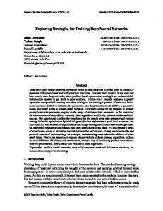
Fig. 1. The α (left), β (middle) and αβ (right) values for a given utterance. The horizonal axis corresponds to the frames of the utterance, while the vertical axis represents the states (phonemes)

audio training data set several times. A speciality of this training method is that we process a whole utterance at a time instead of using just fixed-sized batches of it; however, we only need the correct transcription of the utterance, and do not require any time-alignment. The CTC training method is built on the dynamic search method called forward-backward search [6], which is a standard part of HMM training. The forward-backward algorithm not only gives the optimal path, but at the same time we also get the probability of going through the given phoneme of the transcription for all the frames of the utterance. From this, for each frame, we can calculate a probability distribution over the possible phonemes; then these values can be used as target values when training the acoustic classifier. 2.1

The Forward-Backward Algorithm

Let us begin with the formal description of the forward-backward algorithm. First, let us take the utterance with length T , and let its correct transcription be z = z1 z2 . . . zn . We will also use the output vectors y t of the neural network trained in the previous iteration. α(t, u) can be defined as the summed probability of outputting the u-long prefix of z up to the time index t ≤ T . The initial conditions formulate that the correct sequence starts with the first label in z: 1 yz1 if u = 1, α(1, u) = (1) 0 if u ≥ 2. Now the forward variables at time t can be calculated recursively from those at time t − 1; we can remain in state zu−1 , or move on to the next one (zu ). Thus, t yzu α(t − 1, u) if u = 1, α(t, u) = (2) yzt u α(t − 1, u) + α(t − 1, u − 1) otherwise. In the backward phase we calculate the backward variables β(u, t), which represent the probability of producing the suffix of z having length n − u starting from the frame t + 1. The backward variables can be calculated recursively as 1 if u = n, β(T, u) = (3) 0 otherwise,

84


and for each t < T β(t, u) =

yzt u β(t + 1, u) yzt u β(t + 1, u) + β(t + 1, u + 1)

if u = n, otherwise.

(4)

Fig. 1. illustrates the forward variables, the backward variables and their product for a short utterance. 2.2

Using the αβ values for ANN training

The α(t, u)β(t, u) product values express the overall probability of two factors, summed along all paths: the first is that we recognize the correct sequence of phonemes, and the second is that at frame t we are at the uth phoneme of z. For neural network training, however, we would need a distribution over the phoneme set for frame t. It is not hard to see that such a distribution over the phonemes of z can be obtained by normalizing the α(t, u)β(t, u) products so that they sum up to one (by which step we eliminate the probability of recognizing the correct sequence of phonemes). Then, to normalize this distribution to one over the whole set of phonemes, we need to sum up the scores belonging to the multiple occurrences of the same phonemes in z. That is, the regression targets for any frame t and phoneme ph can be defined by the formula α(t, i)β(t, i) i:zi =ph n i=1

α(t, i)β(t, i)

.

(5)

We can use these values as training targets instead of the standard binary zeroor-one targets with any gradient-based non-linear optimization algorithm. Here, we applied the backpropagation algorithm. 2.3

Garbage Label

Although the above training method may work well for the original phoneme set, Graves et al. introduced a new label (which we will denote by X ), by which the neural network may choose not to omit any phoneme. This label can be inserted between any two phonemes, but of course it can also be skipped. They called this label “blank”, but we consider the term “garbage” more logical. To interpret the role of this label, let us consider a standard tri-state model. This divides each phone into three parts. The middle state corresponds to the steady-state part of the given phone, whereas the beginning and end states represent those parts of the phone which are affected by coarticulation with the preceding and the subsequent phones, respectively. By introducing label X , we allow the system to concentrate on the recognition of the cleanly pronounced middle part of a phone, and it can map the coarticulated parts to the symbol X . Therefore, we find it more logical to use the term garbage label instead of blank, as the latter would suggest that the label X covers silences, but in fact this label more likely corresponds to the coarticulated parts of phones.


85

Formally, introducing this label means that instead of the phoneme sequence z we will use the sequence z = X z1 X z2 X . . . X zn X . The forward-backward algorithm also has to be modified slightly: the initial α values will be set to 1 yz if u = 1 or u = 2, 1 α(1, u) = (6) 0 if u ≥ 3, while for the latter labels we allow skipping the X states: ⎧ t − 1, u) ⎨ yzu α(t α(t, u) = yzt u α(t − 1, u) + α(t − 1, u − 1) ⎩ t yzu α(t − 1, u) + α(t − 1, u − 1) + α(t − 1, u − 2)

if u = 1, if zu = X , otherwise. (7)

The calculation of the β values is performed in a similar way. It is also possible to use the garbage label with a tri-state model: then X is inserted between every state of all the phonemes, while still being optional. 2.4

Decoding

When using Recurrent Neural Networks, it is obvious that we cannot perform a standard Viterbi beam search for decoding. However, when we switch to a standard feed-forward neural network architecture, this constraint vanishes and we can apply any kind of standard decoding method. The only reason we need to alter the decoding part is that we need to remove the garbage label from the resulting phoneme sequence. Luckily, in other respects it does not affect the strictly-interpreted decoding part. This label also has to be ignored during search when we apply a language model like a phoneme n-gram. In our tests we used our own implementation of the Viterbi algorithm [6].

3 3.1

Experiments and Results Databases

We tested the CTC training method on three databases. The first was the wellknown TIMIT set [7], which is frequently used for evaluating the phoneme recognition accuracy of a new method. Although it is a small dataset by today’s standards, a lot of experimental results have been published for it; also, due to its relatively small size, it is ideal for experimentation purposes. We used the standard (core) test set, and withheld a small part of the training set for development purposes. The standard phoneme set consists of 61 phonemes, which is frequently reduced to a set of 39 labels when evaluating; we experimented with training on these 61 phonemes and also on the restricted set of 39 phonemes. The next database was a Hungarian audiobook; our choice was the collection of short stories by Gyula Kr´ udy [9] called “The Travels of Szindbád”, presented by actor S´ andor G´ asp´ ar. The total duration of the audiobook was 212 minutes. From the ten short stories, seven were used for training (164 minutes), one for

86

T. Gr´ osz, G. Gosztolya, and L. T´ oth Table 1. The accuracy scores got for the three different DRN training methods Database

Method Monostate (39)

TIMIT

Monostate (61)

Tristate (183)

CTC + DRN Hand-labeled Forced Alignment CTC + DRN Hand-labeled Forced Alignment CTC + DRN Hand-labeled Forced Alignment

Dev. set 73.31% 72.74% 72.90% 73.93% 73.58% 74.08% 76.80% 77.25% 77.22%

Test set 71.40% 70.65% 71.08% 72.66% 72.06% 72.45% 75.59% 75.30% 75.52%

development (22 minutes) and two for testing (26 minutes) purposes. A part of the Hungarian broadcast news corpus [12] was used as the third database. The speech data of Hungarian broadcast news was collected from eight Hungarian TV channels. The training set was about 5.5 hours long, a small part (1 hour) was used for validation purposes, and a 2-hour part was used for testing. 3.2

Experimental Setup

As the frame-level classifier we utilized Deep Rectifier Neural Networks (DRN) [2,11], which have been shown to achieve state-of-the-art performance on TIMIT [10]. DRN differ from traditional deep neural networks in that they use rectified linear units in the hidden layers; these units differ from standard neurons only in their activation function, where they apply the rectifier function (max(0, x)) instead of the sigmoid or hyperbolic tangent activation. This activation function allows us to build deep networks with many hidden layers without the need for complicated pre-training methods, just by applying standard backpropagation training. Nevertheless, to keep the weights from growing without limit, we have to use some kind of regularization technique; we applied L2 normalization. Our DRN consisted of 5 hidden layers, with 1000 rectifier neurons in each layer. The initial learn rate was set to 0.2 and held fixed while the error on the development set kept decreasing. Afterwards, if the error rate did not decrease for a given iteration, the learn rate was subsequently halved. The learning was accelerated by using a momentum value of 0.9. We used the standard MFCC+Δ+ΔΔ feature set, and trained the neural network on 15 neighbouring frames, so the number of inputs to the acoustic model totalled 585. We did not apply any language model, as we wanted to focus on the acoustic model. Furthermore, due to the presence of the garbage symbol in the phoneme set, including a phoneme n-gram in the dynamic search method is not trivial; of course, we plan to implement this small modification in the near future. 3.3

Results

First we evaluated the CTC training method on the TIMIT database, the results of which can be seen in Table 1. As for this data set a manual segmentation is


87

Table 2. The accuracy scores got for the two different DRN training methods Database

Method Monostate (52)

Audiobook Tristate (156) Monostate (52) Broadcast news Tristate (156)

CTC + DRN Forced Alignment CTC + DRN Forced Alignment CTC + DRN Forced Alignment CTC + DRN Forced Alignment

Dev. set 82.15% 82.24% 87.42% 87.53% 74.04% 74.18% 78.38% 77.87%

Test set 83.45% 83.02% 88.33% 88.04% 74.42% 74.36% 78.77% 78.26%

also available, the results obtained by training using the manually given boundaries is used as a baseline. As a further comparison, the training was repeated in the usual way, where the training labels are obtained using forced alignment. We found that the results obtained using the hand-labeled set of labels were noticeably worse than the ones we got when we used forced-aligned labels. This reflects the fact that the manually placed phone boundaries are suboptimal compared to the case where the algorithm is allowed to re-align the boundaries according to its needs. The results obtained using tri-state models were always better than those got with monostate ones, on all three databases. Furthermore, the CTC DRN training model consistently outperformed the other two tested training schemes (although sometimes only slightly), when evaluated on the test set. On the development set usually the standard training strategies were better, which can probably be attributed to overfitting. Training when using CTC was slightly slower than in the baseline cases: calculating the α and β values increased the execution times only by a very small amount, but it took a few more iterations to make the weights converge. On TIMIT, CTC used all training vectors 24-25 times, whereas it was 18-19 in the baseline cases. This is probably due to that CTC strongly relies on the acoustic classifier trained in the previous iteration, so it takes a few iterations before the training starts to converge. We think these values are not high, especially as Graves et al. reported much higher values (frequently over 100) [4]. Another interesting point is that besides the similar accuracy scores, standard backpropagation leads to a relatively high number of phoneme insertions, while when performing CTC it is common to have a lot of deletion errors. The reason is that the correct phonemes are often suppressed by X s, which labels are then deleted from the result before the accuracy score is calculated. This behaviour, however, does not affect the overall quality of the result.

4

Conclusions

In this study we adapted a sequence learning method (which was developed for Recurrent Neural Networks) to a standard HMM/ANN architecture. Compared to standard zero-or-one frame-level backpropagation ANN training we found that

88


networks trained with this sequence learning method always produced higher accuracy scores than the baseline ones. In the future we plan to implement a duration model, incorporate a phoneme bigram as language model, and combine the method with a convolutional network to further improve its performance. Acknowledgments. This publication is supported by the European Union and co-funded by the European Social Fund. Project title: Telemedicine-oriented research activities in the fields of mathematics, informatics and medical sciences. ´ Project number: TAMOP-4.2.2.A-11/1/KONV-2012-0073.

References 1. Bourlard, H.A., Morgan, N.: Connectionist Speech Recognition: A Hybrid Approach. Kluwer Academic, Norwell (1993) 2. Glorot, X., Bordes, A., Bengio, Y.: Deep sparse rectifier networks. In: Proceedings of AISTATS, pp. 315–323 (2011) 3. Graves, A.: Supervised Sequence Labelling with Recurrent Neural Networks. SCI, vol. 385. Springer, Heidelberg (2012) 4. Graves, A., Mohamed, A.R., Hinton, G.E.: Speech recognition with Deep Recurrent Neural Networks. In: Proceedings of ICASSP, pp. 6645–6649 (2013) 5. Hinton, G., Deng, L., Yu, D., Dahl, G., Mohamed, A., Jaitly, N., Senior, A., Vanhoucke, V., Nguyen, P., Sainath, T., Kingsbury, B.: Deep Neural Networks for acoustic modeling in Speech Recognition. IEEE Signal Processing Magazine 29(6), 82–97 (2012) 6. Huang, X., Acero, A., Hon, H.W.: Spoken Language Processing. Prentice Hall (2001) 7. Lamel, L., Kassel, R., Seneff, S.: Speech database development: Design and analysis of the acoustic-phonetic corpus. In: DARPA Speech Recognition Workshop, pp. 121–124 (1986) 8. Senior, A., Heigold, G., Bacchiani, M., Liao, H.: GMM-free DNN training. In: Proceedings of ICASSP, pp. 5639–5643 (2014) 9. T´ oth, L., Tarj´ an, B., S´ arosi, G., Mihajlik, P.: Speech recognition experiments with audiobooks. Acta Cybernetica, 695–713 (2010) 10. T´ oth, L.: Convolutional deep rectifier neural nets for phone recognition. In: Proceedings of Interspeech, Lyon, France, pp. 1722–1726 (2013) 11. T´ oth, L.: Phone recognition with Deep Sparse Rectifier Neural Networks. In: Proceedings of ICASSP, pp. 6985–6989 (2013) 12. T´ oth, L., Gr´ osz, T.: A comparison of deep neural network training methods for large vocabulary speech recognition. In: Proceedings of TSD, pp. 36–43 (2013) 13. Werbos, P.J.: Backpropagation Through Time: what it does and how to do it. Proceedings of the IEEE 78(10), 1550–1560 (1990)