A Sequent Calculus for Type Theory Long version - CiteSeerX

A Sequent Calculus for Type Theory Long version Stéphane Lengrand1,2 , Roy Dyckhoff1 , and James McKinna1 1

School of Computer Science, University of St Andrews, Scotland. 2 PPS, Université Paris 7, France. {sl,rd,james}@dcs.st-and.ac.uk 3rd May 2006

Abstract Based on natural deduction, Pure Type Systems (PTS) can express a wide range of type theories. In order to express proof-search in such theories, we introduce the Pure Type Sequent Calculi (PTSC) by enriching a sequent calculus due to Herbelin, adapted to proof-search and strongly related to natural deduction. PTSC are equipped with a normalisation procedure, adapted from Herbelin’s and defined by local rewrite rules as in Cut-elimination, using explicit substitutions. It satisfies Subject Reduction and it is confluent. A PTSC is logically equivalent to its corresponding PTS, and the former is strongly normalising if and only if the latter is. We show how the conversion rules can be incorporated inside logical rules (as in syntaxdirected rules for type checking), so that basic proof-search tactics in type theory are merely the root-first application of our inference rules. keywords: Type theory, PTS, sequent calculus, proof-search, strong normalisation

Introduction In this paper, we apply to the framework of Pure Type Systems [Bar92] the insights into the relationship between sequent calculus and natural deduction as developed in previous papers by Herbelin [Her94,Her95], the second author and others [DP99b,PD00,DU03]. In sequent calculus the proof-search space is often the cut-free fragment, since the latter usually satisfies the subformula property. Herbelin’s sequent calculus LJT has the extra advantage of being closer to natural deduction, in that it is permutation-free, and it makes proof-search more deterministic than a Gentzenstyle sequent calculus. This makes LJT a natural formalism to organise proofsearch in intuitionistic logic [DP99a], and, its derivations being close to the notion of uniform proofs, LJT can be used to describe proof-search in pure Prolog and some of its extensions [MNPS91]. The corresponding term assignment system also expresses the intimate details of β-normalisation in λ-calculus in a form closer to abstract (stack-based) machines for reduction (such as Krivine’s [Kri]). The framework of Pure Type Systems (PTS) [Bar92] exploits and generalises the Curry-Howard correspondence, and accounts for many systems already existing, starting with Barendregt’s Cube. Proof assistants based on them, such as the Coq system [Coq] or the Lego system [LP92], feature interactive proof construction methods using proof-search tactics. Primitive tactics display an asymmetry

between introduction rules and elimination rules of the underlying natural deduction calculus: the tactic Intro corresponds to the right-introduction rule for the Π-type (whether in natural deduction or in sequent calculus), but the tactics Apply in Coq or Refine in Lego are much closer (in spirit) to the left-introduction of Π-types (as in sequent calculus) than to elimination rules of natural deduction. Although encodings from natural deduction to sequent calculus and vice-versa have been widely studied [Gen35,Pra65,Zuc74], the representation in sequent calculus of type theories is relatively undeveloped compared to the literature about type theory in natural deduction. An interesting approach to Pure Type Systems using sequent calculus is in [GR03]. Nevertheless, only the typing rules are in a sequent calculus style, whereas the syntax is still in a natural deduction style: in particular, proofs are denoted by λ-terms, the structure of which no longer matches the structure of proofs. However, proofs in sequent calculus can be denoted by terms; for instance, a construction M · l, representing a list of terms with head M and tail l, is introduced in [Her94,Her95] to denote the left-introduction of implication (in the sequent calculus LJT): Γ ` M :A Γ; B ` l:C Γ; A → B ` M · l:C This approach is extended to the corner of the Cube with dependent types and type constructors in [PD00], but types are still built with λ-terms, so that the system extensively uses conversion functions from sequent calculus to natural deduction and back. With such term assignment systems, cut-elimination can be done by means of a rewrite system so that the cut-free proofs are denoted by terms in normal form. In type theory, not only is the notion of proof-normalisation/cut-elimination interesting on its own, but it is even necessary to define the notion of typability, as soon as types depend on terms. In this paper we enrich Herbelin’s sequent calculus LJT into a a collection of systems called Pure Type Sequent Calculi (PTSC), capturing the traditional PTS, with the hope to improve the understanding of implementation of proof systems based on PTS in respect of: – a direct analysis of the basic tactics, which could then be moved into the kernel, rather than requiring a separate type-checking layer for correctness, – opening the way to improve the basic system with an approach closer to abstract machines to express reductions, both in type-checking and in execution (of extracted programs), – studying extensions to systems involving inductive types/families (such as the Calculus of Inductive Constructions). Inspired by the fact that, in type theory, implication and universal quantification are just a dependent product, we modify the inference rule above to obtain 2

the left-introduction rule for a Π-type in a PTSC: Γ ` M : A Γ ; hM/xiB ` l : C Πl Γ ; ΠxA .B ` M · l : C Derivability of sequents in a PTSC is denoted by `, while derivability in a PTS is denoted by `PTS . We establish the logical equivalence between a PTSC and its corresponding PTS by means of type-preserving encodings. We also prove that the former is strongly normalising if and only if the latter is. The proof is based on mutual encodings that allow the normalisation procedure of one formalism to be simulated by that of the other. Part of the proof also uses a technique by Bloo and Geuvers [BG99], introduced to prove strong normalisation properties of an explicit substitution calculus and later used in [DU03]. In order to show the convenience for proof-search of the sequent calculus approach, we then present a system that is syntax-directed for proof-search, by incorporating the conversion rules into the typing rules that correspond to term constructions. This incorporation is similar to the constructive engine of [Hue89], but different in that proof search takes Γ and A as inputs and produces a (normal) term M such that Γ ` M : A, while the constructive engine takes Γ and M as inputs and produces A. Derivability in the proof-search system is denoted by `PS . Section 1 presents the syntax of a PTSC and gives the rewrite rules for normalisation. Section 2 gives the typing system with the parameters specifying the PTSC, and a few properties are stated such as Subject Reduction. Section 3 establishes the correspondence between a PTSC and its corresponding PTS, from which we derive the confluence. Section 4 presents the strong normalisation result. Section 5 discusses proof-search in a PTSC.

1

Syntax and operational semantics of a PTSC

The syntax of a PTSC depends on a given set S of sorts, written s, s0 , . . ., and a denumerable set X of variables, written x, y, z, . . .. The set T of terms (denoted M, N, P, . . .) and the set L of lists (denoted l, l0 , . . .) are inductively defined as M, N, A, B ::= ΠxA .B | λxA .M | s | x l | M l | hM/xiN l, l0 ::= [] | M · l | l@l0 | hM/xil ΠxA .M , λxA .M , and hN/xiM bind x in M , and hM/xil binds x in l, thus defining the free variables of terms and lists as well as α-conversion. We use Barendregt’s convention that no variable is free and bound in a term in order to avoid variable capture when reducing it. Let A → B denote ΠxA .B when x 6∈ FV(B). This syntax is an extension of Herbelin’s λ [Her95] (with type annotations on λ-abstractions). Lists are used to represent series of arguments of a function, the terms x l (resp. M l) representing the application of x (resp. M ) to the list of arguments l. Note that a variable alone is not a term, it has to be applied to a 3

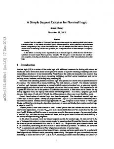
list, possibly the empty list, denoted []. The list with head M and tail l is denoted M · l, with a typing rule corresponding to the left-introduction of Π-types (c.f. Section 2). Successive applications give rise to the concatenation of lists, denoted l@l0 , and hM/xiN and hM/xil are explicit substitution operators on terms and lists, respectively. They will be used in two ways: first, to instantiate a universally quantified variable, and second, to describe explicitly the interaction between the constructors in the normalisation process, which is adapted from [DU03] and shown in Fig. 1. Side-conditions to avoid variable capture can be inferred from the reduction rules and are ensured by Barendregt’s convention. Confluence of the system is proved in section 3. More intuition about Herbelin’s calculus, its syntax and operational semantics is given in [Her95]. (λxA .M ) (N · l) −→ (hN/xiM ) l

B                          

B1 B2 B3 A1 A2  A3 C1     C2 x       C3           C4    xsubst: C5       C6          D1         D2      D3

M [] −→ M 0 (x l) l −→ x (l@l0 ) 0 (M l) l −→ M (l@l0 ) (M · l0 )@l −→ M · (l0 @l) []@l −→ l (l@l0 )@l00 −→ l@(l0 @l00 ) hP/yiλxA .M −→ λxhP/yiA .hP/yiM hP/yi(y l) −→ P hP/yil hP/yi(x l) −→ x hP/yil if x 6= y hP/yi(M l) −→ hP/yiM hP/yil hP/yiΠxA .B −→ ΠxhP/yiA .hP/yiB hP/yis −→ s hP/yi[] −→ [] hP/yi(M · l) −→ (hP/yiM ) · (hP/yil) hP/yi(l@l0 ) −→ (hP/yil)@(hP/yil0 )

Figure 1. Reduction Rules We denote by −→G the contextual closure of the reduction relation defined by any system G of rewrite rules (such as B, xsubst, x). The transitive closure of −→G is denoted by −→+ G , its reflexive and transitive closure is denoted by −→∗ G , and its symmetric reflexive and transitive closure is denoted by ←→∗ G . The set of strongly normalising elements (those from which no infinite −→G reduction sequence starts) is SNG . When not specified, G is assumed to be the system B, x from Fig. 1. We now show that system x is terminating. If we add rule B, then the system fails to be terminating unless we only consider terms that are typed in a particular typing system. 4

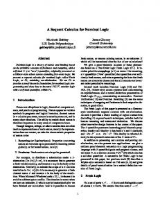
We encode terms and lists into a first-order syntax given by the following signature: ?, i(_), ii(_, _), cut(_, _), sub(_, _) We equip this signature with the well-founded precedence relation defined by ? ≺ i(_) ≺ ii(_, _) ≺ cut(_, _) ≺ sub(_, _) The lexicographic path ordering (lpo) induces on the first-order terms is also wellfounded (definitions and results can be found in [KL80]). The encoding aforementioned is given in Fig 2. S(s) =? S(λxA .M ) = S(ΠxA .M ) = ii(S(A), S(M )) S(x l) = i(S(l)) S(M l) = cut(S(M ), S(l)) S(hM/xiN ) = sub(S(M ), S(N )) S([]) =? S(M · l) = ii(S(M ), S(l)) S(l@l0 ) = ii(S(l), S(l0 )) S(hM/xiN ) = sub(S(M ), S(l)) Figure 2. First-order encoding

Theorem 1. If M −→x S(l) >lpo S(l0 ).

M 0 then S(M ) >lpo S(M 0 ), and if l −→x

l0 then

Proof. By induction on M, l. Corollary 1. System x is terminating (on all terms and lists).

2

Typing system and properties

Given the set of sorts S, a particular PTSC is specified by a set A ⊆ S 2 and a set R ⊆ S 3 . We shall see an example in section 4. Definition 1 (Environments). – Environments are lists of pairs from X × T denoted (x : A). – We define the domain of an environment and the application of a substitution to an environment as follows: Dom([]) = ∅ hP/yi([]) = []

Dom(Γ, (x : A)) = Dom(Γ ) ∪ {x} hP/yi(Γ, (x : A)) = hP/yiΓ, (x : hP/yiA) 5

Γ ` A:s

empty [] wf (s, s0 ) ∈ A

Γ wf

Γ ` A : s1

Γ, (x : A) ` B : s2

Γ, (x : A) ` M : B

Γ ` λxA .M : ΠxA .B Γ ` M :A

Γ ` B :s

Γ; A ` l:B

Πr

A←→∗ B

Γ ; C ` l0 @l : B Γ ` M :A

Γ; A ` l:B

Γ ` M l:B

Γ ` A:s

Selectx

Γ ` ΠxA .B : s

convr

axiom

Γ ; A ` [] : A

Γ ` M :A

Γ ; hM/xiB ` l : C

A

Πl

Γ ; Πx .B ` M · l : C

Γ ` B :s

Γ; A ` l:B

(x : A) ∈ Γ

Γ ` x l:B

A←→∗ B

Γ; C ` l:B Γ ; C ` l0 : A

Πwf

Γ ` Πx .B : s3

Γ ` M :B Γ; C ` l:A

(s1 , s2 , s3 ) ∈ R

A

Γ ` s:s Γ ` ΠxA .B : s

extend

Γ, (x : A) wf

sorted

0

x∈ / Dom(Γ )

Cut1

Cut3

Γ; A ` l:C

conv0r

A←→∗ B

Γ ` B :s

convl

Γ; B ` l:C

Γ ` P :A

Γ, (x : A), ∆; B ` l : C

Γ, hP/xi∆ v ∆0 wf

∆0 ; hP/xiB ` hP/xil : hP/xiC Γ ` P :A

Γ, (x : A), ∆ ` M : C

Cut2

Γ, hP/xi∆ v ∆0 wf

Cut4 ∆0 ` hP/xiM : C 0 where either (C 0 = C ∈ S) or C 6∈ S and C 0 = hP/xiC

Figure 3. Typing rules of a PTSC

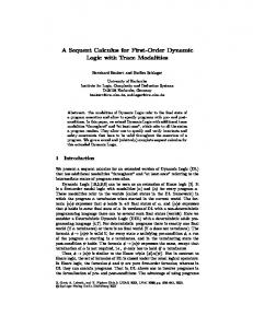
– We define the following inclusion relation between environments: Γ v ∆ if for all (x : A) ∈ Γ , there is (x : B) ∈ ∆ with A←→∗ B The inference rules in Fig. 3 inductively define the derivability of three kinds of judgement: some of the form Γ wf, some of the form Γ ` M : A and some of the form Γ ; B ` l : A. In the latter case, B is said to be in the stoup of the sequent. Side-conditions are used, such as (s1 , s2 , s3 ) ∈ R, x 6∈ Dom(Γ ), A←→∗ B or ∆ v Γ , and we use the abbreviation ∆ v Γ wf for ∆ v Γ and Γ wf. There are three conversion rules convr , conv0r , and convl in order to deal with the two kinds of judgements and, for one of them, convert the type in the stoup. Since the substitution of a variable in an environment affects the rest of the environment (which could depend on the variable), the two rules for explicit substitutions (Cut2 and Cut4 ) must have a particular shape that manipulates the environment, if the PTSC is to satisfy basic required properties like those of a PTS. The lemmas of this section are proved by induction on typing derivations: Lemma 1 (Properties of typing judgements). If Γ ` M : A (resp. Γ ; B ` l : C) then FV(M ) ⊆ Dom(Γ ) (resp. FV(l) ⊆ Dom(Γ )), and the following judgements can be derived with strictly smaller typing derivations: 6

1. Γ wf 2. Γ ` A : s for some s ∈ S, unless A ∈ S (resp. Γ ` B : s and Γ ` C : s0 for some s, s0 ∈ S) Corollary 2 (Properties of well-formed environments). 1. If Γ, x : A, ∆ wf then Γ ` A : s for some s ∈ S with x 6∈ Dom(Γ, ∆) and FV(A) ⊆ Dom(Γ ) (and in particular x 6∈ FV(A)) 2. If Γ, ∆ wf then Γ wf. Lemma 2 (Weakening). Suppose Γ, Γ 0 wf and Dom(Γ 0 ) ∩ Dom(∆) = ∅. 1. If Γ, ∆ ` M : B then Γ, Γ 0 , ∆ ` M : B. 2. If Γ, ∆; C ` l : B, then Γ, Γ 0 , ∆; C ` l : B. 3. If Γ, ∆ wf, then Γ, Γ 0 , ∆ wf. We can also strengthen the weakening property into the thinning property by induction on the typing derivation. This allows to weaken the environment, change its order, and convert the types inside, as long as it remains well-formed: Lemma 3 (Thinning). Suppose Γ v Γ 0 wf and Dom(Γ 0 ) ∩ Dom(∆) = ∅. 1. If Γ, ∆ ` M : B then Γ 0 , ∆ ` M : B. 2. If Γ, ∆; C ` l : B, then Γ 0 , ∆; C ` l : B. 3. If Γ, ∆ wf, then Γ 0 , ∆ wf. Using all of the results above, Subject Reduction can be proved (see the Appendix). Theorem 2 (Subject Reduction in a PTSC). 1. If Γ ` M : A and M −→ M 0 , then Γ ` M 0 : A 2. If Γ ; A ` l : B and l −→ l0 , then Γ ; A ` l0 : B

3

Correspondence with Pure Type Systems

There is a logical correspondence between a PTSC given by the sets S, A and R and the PTS given by the same sets. We briefly recall the syntax and semantics of the PTS. The terms have the following syntax: t, u, v, T, U, V, . . . ::= x | s | ΠxT .t | λxT .t | t u which is equipped with the β-reduction rule (λxv .t) u −→β t{x = u}, in which the substitution is implicit, i.e. is a meta-operation. The terms are typed by the typing rules in Fig. 3, which depend on the sets S, A and R. PTS are confluent and satisfy the following properties (e.g. [Bar92]): 7

Γ `PTS T : s [] wf Γ wf

x∈ / Dom(Γ )

Γ wf

Γ, (x : T ) wf

(s, s0 ) ∈ A

(x : T ) ∈ Γ

Γ `PTS x : T

Γ `PTS U : s1

Γ, (x : U ) `PTS T : s2

(s1 , s2 , s3 ) ∈ R

U

0

Γ `PTS Πx .T : s3

Γ `PTS s : s

Γ `PTS ΠxU .V : s

Γ, (x : U ) `PTS t : V

Γ `PTS t : ΠxT .U

Γ `PTS λxU .t : ΠxU .V Γ `PTS t : U

Γ `PTS u : T

Γ `PTS t u : U {x = u} Γ `PTS V : s

U ←→∗ β V

Γ `PTS t : V

Figure 4. Typing rules of a PTS Theorem 3. 1. If Γ `PTS t : u and Γ v ∆ wf then ∆ `PTS t : u (where the relation v is defined similarly to that of PTSC, but with β-equivalence). 2. If Γ `PTS t : v and Γ, y : v, ∆ `PTS u : v 0 then Γ, ∆{y = t} `PTS u{y = t} : v 0 {y = t}. 3. If Γ `PTS t : v and t −→β u then Γ `PTS u : v. In order to encode the syntax of a PTS into that of a PTSC, it is convenient re-express the syntax of a PTS with a grammar closer to that of a PTSC as follows: w ::= s | ΠxT .U | λxT .t − → − → t, u, v, T, U, V, . . . ::= w | x t | w u t − → where t represents a list of “t-terms” of arbitrary length. The grammar is sound and complete with respect to the usual one presented at the begining of the section, and it has the advantage of isolating redexes in one term construction in a way similar to a PTSC. Given in the left-hand side of Fig. 5, the encoding into the corresponding PTSC, is threefold: hw applies to “w-terms”, h applies to “t-terms”, and hl to lists of “t-terms”. The right-hand side of Fig. 5 shows the encoding from a PTSC to a PTS. We prove the following theorem by induction on t and M : Theorem 4 (Properties of the encodings). 1. 2. 3. 4. 5. 6.

h(t) is always an x-normal form, and hh(t)/xih(u)−→∗ x h(u{x = t}). k(h(t)) = t If M is an x-normal form, then M = h(k(M )) M −→∗ x h(k(M )) If t −→β u then h(t)−→+ h(u) If M −→ N then k(M )−→∗ β k(N ) 8

hw (s) =s v 0 hw (Πx .v ) = Πxh(v) .h(v 0 ) hw (λxv .t) = λxh(v) .h(t) h(w) = hw (w) − → → − h(x t ) = x hl ( t ) − → − → h(w u t ) = hw (w) (h(u) · hl ( t )) − → hl ( ∅ ) = [] −.−.−.−→ −−−−→ hl (− u− u ) = h(u1 ) · hl (− u− 1 i 2 . . . ui ) From a PTS to a PTSC

k(ΠxA .B) = Πxk(A) .k(B) k(λxA .M ) = λxk(A) .k(M ) k(s) =s k(x l) = kz (l){z = x} z z k(M l) = k (l){z = k(M )} z k(hP/xiM ) = k(M ){x = k(P )} ky ([]) =y y k (M · l) = kz (l){z = y k(M )} z ky (l@l0 ) = kz (l0 ){z = ky (l)} z ky (hP/xil) = ky (l){x = k(P )} From a PTSC to a PTS

fresh fresh

fresh fresh

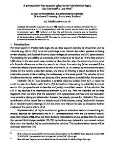
Figure 5. Mutual encodings between a PTS and a PTSC Now we use Theorem 4 to prove the confluence of PTSC and the equivalence of the equational theories. Corollary 3 (Confluence). −→x is confluent and −→ is confluent. Proof: We use the technique of simulation as for instance in [KL05]: consider two reduction sequences starting from a term in a PTSC. They can be simulated through k by β-reductions, and since a PTS is confluent, we can close the diagram. Now the lower part of the diagram can be simulated through h back in the PTSC, which closes the diagram there as well. The diagram is shown in Fig. 6. Notice that the proof of confluence has nothing to do with typing and does not rely on any result in section 2 (in fact, we use confluence in the proof of Subject Reduction in the Appendix). 2

Corollary 4 (Equational theories). t←→∗ β u if and only if h(t)←→∗ h(u) M ←→∗ N if and only if k(M )←→∗ β k(N ) Regarding typing, we first define the following operations on environments: h([]) = [] h(Γ, (x : v)) = h(Γ ), (x : h(v))

k([]) = [] k(Γ, (x : A)) = k(Γ ), (x : k(A))

9

N1

N LLL rr LLL ∗ r r ∗ rr LLL r r LLL r r r & rx k

N2

®¶

k

®¶

s ∗ sss s ss sy s

k(N1 ) h

k(N ) K

LL LL ∗ LL LL LL %

KK KK∗ KK KK %

k

®¶

k(N2 )

M

r ∗ rrr rr r r ry r

®¶

h

®¶

h(k(N1 )) K

KK KK K ∗ KKK %

h

®¶

h(M )

h(k(N2 ))

s ss ss s s ∗ sy s

Figure 6. Proof of confluence Preservation of typing is proved by induction on the typing derivations: Theorem 5 (Preservation of typing 1). 1. If Γ `PTS t : T then h(Γ ) ` h(t) : h(T ) 2. If (Γ `PTS ti : Ti {x1 = t1 } . . . {xi−1 = ti−1 })i=1...n and h(Γ ) ` h(Πx1 T1 .. . . Πxn Tn .T ) : s then h(Γ ); h(Πx1 T1 .. . . Πxn Tn .T ) ` hl (t1 . . . tn ) : h(T {x1 = t1 } . . . {xn = tn }) 3. If Γ wf then h(Γ ) wf Theorem 6 (Preservation of typing 2). 1. If Γ ` M : A then k(Γ ) `PTS k(M ) : k(A) 2. If Γ ; B ` l : A then k(Γ ), y : k(B) `PTS ky (l) : k(A) for a fresh y 3. If Γ wf then k(Γ ) wf

4

Equivalence of Strong Normalisation

Theorem 7. A PTSC given by the sets S, A, and R is strongly normalising if and only if the PTS given by the same sets is.

10

Proof: Assume that the PTSC is strongly normalising, and let us consider a welltyped t of the corresponding PTS, i.e. Γ `PTS t : T for some Γ, T . By Theorem 5, h(Γ ) ` h(t) : h(T ) so h(t) ∈ SN. Now by Theorem 4, any reduction sequence starting from t maps to a reduction sequence of at least the same length starting from h(t), but those are finite. Now assume that the PTS is strongly normalising and that Γ ` M : A in the corresponding PTSC. By subject reduction, any N such that M −→∗ N satisfies Γ ` N : A and any sub-term P (resp. sub-list l) of any such N is also typable. By Theorem 6, for any such P (resp. l), k(P ) (resp. ky (l)) is typable in the PTS, so it is strongly normalising by assumption. Following Bloo and Geuvers’ technique from [BG99], we now refine the firstorder encoding defined in section 1 of any such P and l . We refine the first-order signature by labeling the symbols cutt (_, _) and subt (_, _) with all strongly normalising terms t of a PTS, thus generating an infinite signature. The precedence relation is refined as follows ? ≺ i(_) ≺ ii(_, _) ≺ cutt (_, _) ≺ subt (_, _) but we also set subt (_, _) ≺ cutt (_, _) whenever t0 −→+ β t. The precedence is still well-founded, so the induced (lpo) is also still well-founded (definitions and results can be found in [KL80]). The refinement of the encoding is given in Fig 7. An induction on terms shows that reductions decrease the lpo. 2 0

T (s) =? A A T (λx .M ) = T (Πx .M ) = ii(T (A), T (M )) T (x l) = i(T (l)) T (M l) = cutk(M l) (T (M ), T (l)) T (hM/xiN ) = subk(hM/xiN ) (T (M ), T (N )) T ([]) =? T (M · l) = ii(T (M ), T (l)) T (l@l0 ) = ii(T (l), T (l0 )) T (hM/xiN ) = subk(hM/xil) (T (M ), T (l)) Figure 7. First-order encoding Examples of strongly normalising PTS are the Calculus of Constructions [CH88], on which the proof-assistant Coq is based [Coq] (but it also uses inductive types and local definitions), as well as all the other systems of Barendregt’s Cube, for all of which we now have a corresponding PTSC that can be used for proof-search. 11

5

Proof-search

In contrast to propositional logic where cut is an admissible rule of sequent calculus, terms in normal form may need a cut-rule in their typing derivation. For instance in rule Πl, a type which is not normalised (hM/xiB) must appear in the stoup of the third premiss, so that cuts might be needed to type it inside the derivation. We conjecture that if we modify rule Πl by now requiring in the stoup of its third premiss a normal form to which hM/xiB reduces, then any typable normal form can be typed with a cut-free derivation. However, this would make rule Πl more complicated and, more importantly, we do not need this conjecture to hold in order to perform proof-search. Here, the inputs are an environment Γ and a type A, henceforth called goal, and the output is a term M such that Γ ` M : A. When we look for a list, the type in the stoup is also an input. The inference rules now need to be directed by the shape of the goal (or of the type in the stoup), and the proof-search system (PS, for short) can be obtained by optimising the use of the conversion rules as shown in Fig. 8. The incorporation of the conversion rules into the other rules is similar to that of the constructive engine in natural deduction [Hue89,vBJMP94]; however the latter was designed for type synthesis, for which the inputs and outputs are not the same as in proof-search, as mentioned in the introduction.

C−→∗ s0

(s, s0 ) ∈ A

sortedPS

C−→∗ s3

(s1 , s2 , s3 ) ∈ R

Γ, (x : A) `PS B : s2

A

ΠwfPS

Γ `PS Πx .B : C

Γ `PS s : C C−→∗ ΠxA .B

Γ `PS A : s1

A is a normal form

Γ, (x : A) `PS M : B

Γ `PS λxA .M : C D−→∗ ΠxA .B

Γ `PS M : A

ΠrPS

Γ ; hM/xiB `PS l : C

ΠlPS

Γ ; D `PS M · l : C

(x : A) ∈ Γ

Γ ; A `PS l : B

Selectx

Γ `PS x l : B A←→∗ A0 Γ ; A `PS [] : A0

axiomPS

Figure 8. Rules for Proof-search

Notice than in PS there are no cut-rules. Indeed, even though in the original typing system cuts are required in typing derivations of normal forms, they only occur to check that types are well-typed themsleves. Here we removed those type-checking constraints, relaxing the system, because types are the input of proof-search, and they would be checked before starting the search. PS is sound and complete in the following sense: 12

Theorem 8. 1. (Soundness) Provided Γ ` A : s, if Γ `PS M : A then Γ ` M : A. 2. (Completeness) If Γ ` M : A and M is a normal form, then Γ `PS M : A. Proof: Both proofs are done by induction on typing derivations, with similar statements for lists. For Soundness, the type-checking proviso is verified every time we need the induction hypothesis. For Completeness, the following lemma is required (and also proved inductively): assuming A←→∗ A0 and B←→∗ B 0 , if Γ `PS M : A then Γ `PS M : A0 , and if Γ ; B `PS l : A then Γ ; B 0 `PS l : A0 . 2 Note that neither part of the theorem relies on the unsolved problem of expansion postponement [vBJMP94,Pol98]. Indeed, PS does not check types. When recovering a full derivation tree from a PS one by the soundness theorem, expansions and cuts might be introduced at any point, coming from the derivation of the type-checking proviso. Basic proof-search can be done in the proof-search system simply by reducing the goal, or the type in the stoup, and then, depending on its shape, trying to apply one of the inference rules bottom-up. There are three points of non-determinism in proof-search: – The choice of a variable x for applying rule Selectx , knowing only Γ and B (this corresponds in natural deduction to the choice of the head-variable of the proof-term). Not every variable of the environment will work, since the type in the stoup will eventually have to be unified with the goal, so we still need back-tracking. – When the goal reduces to a Π-type, there is an overlap between rules ΠrPS and Selectx ; similarly, when the type in the stoup reduces to a Π-type, there is an overlap between rules ΠlPS and axiomPS . Both overlaps disappear when Selectx is restricted to the case when the goal does not reduce to a Π-type (and sequents with stoups never have a goal reducing to a Π-type). This corresponds to looking only for η-long normal forms in natural deduction. This restriction also brings the derivations in LJT (and in our PTSC) closer to the notion of uniform proofs. Further work includes the addition of η to the notion of conversion in PTSC. – When the goal reduces to a sort s, three rules can be applied (in contrast to the first two points, this source of non-determinism does not already appear in the propositional case). The non-determinism is already present in natural deduction, but the sequent calculus version conveniently identifies where it occurs exactly. We now give the example of a derivation in PS. Consider the PTSC given by: S = {Type, Kind}, A = {(Type, Kind)}, and R = {(Type, Type), (Kind, Type)}. Let A ∧ B stand for ΠQType .(A → (B → Q)) → Q. Trying to find a term M such that A : Type, B : Type ` M : (A ∧ B) → (B ∧ A), we first produce the following PS-derivation (for brevity we omit the types on the λ-abstractions and we abbreviate x [] as x for any variable x): 13

πA axiomPS πB Γ `PS NA : A Γ ; Q `PS [] : Q ΠlPS Γ `PS NB : B Γ ; A → Q `PS NA · [] : Q ΠlPS Γ ; B → (A → Q) `PS NB · NA · [] : Q Selecty Γ `PS y NB · NA · [] : Q ===================================================== ΠrPS A : Type, B : Type `PS λx.λQ.λy.y NB · NA · [] : (A ∧ B) → (B ∧ A) where Γ = A : Type, B : Type, x : A ∧ B, Q : Type, y : B → (A → Q), and πA is the following derivation (NA = x A · (λx0 .λy 0 .x0 ) · []): axiomPS Γ, x0 : A, y 0 : B; A `PS [] : A Selectx0 Γ, x0 : A, y 0 : B `PS x0 : A axiomPS ========0===0==0============= ΠrPS axiomPS Γ ; Type `PS [] : Type Γ `PS λx .λy .x : A → (B → A) Γ ; A `PS [] : A SelectA ΠlPS Γ `PS A : Type Γ ; (A → (B → A)) → A `PS (λx0 .λy 0 .x0 ) · [] : A ΠlPS Γ ; A ∧ B `PS A · (λx0 .λy 0 .x0 ) · [] : A Selectx Γ `PS x A · (λx0 .λy 0 .x0 ) · [] : A and πB is the derivation similar to πA (NB = x B · (λx0 .λy 0 .y 0 ) · []) with conclusion Γ `PS x B · (λx0 .λy 0 .y 0 ) · [] : B. This example shows how the non-determism of proof-search is sometimes quite constrained by the need to eventually unify the type in the stoup with the goal. For instance in πA (resp. πB ), the resolution of Γ ` Q : Type by A (resp. B) could be infered from the unification in the right-hand side branch. In Coq [Coq], the proof-search tactic apply x can be decomposed into the bottom-up application of Selectx followed by a series of bottom-up applications of ΠlPS and finally axiomPS , but it either delays the resolution of sub-goals or automatically solves them from the unification attempt, often avoiding obvious back-tracking. In order to mimic even more closely this basic tactic, delaying the resolution of sub-goals can be done by using meta-variables, to be instantiated later with the help of the unification constraint. By extending PTSC with meta-variables, we can actually go further and express a sound and complete algorithm for type inhabitant enumeration (similar to Dowek’s [Dow93] and Muñoz’s [Mun01] in natural deduction) simply as the bottom-up construction of derivation trees in sequent calculus. Proof-search tactics in natural deduction simply depart from the simple bottomup application of the typing rules, so that their readability and usage would be made more complex. Just as in propositional logic [DP99a], sequent calculi can be a useful theoretical approach to study and design those tactics, in the hope to improve semi-automated reasoning in proof-assistants such as Coq. 14

Conclusion and Further Work We have defined a parameterised formalism that gives a sequent calculus for each PTS. It comprises a syntax, a rewrite system and typing rules. In constrast to previous work, the syntax of both types and proof-terms of PTSC is in a sequentcalculus style, thus avoiding the use of implicit or explicit conversions to natural deduction [GR03,PD00]. A strong correspondence with natural deduction has been established (regarding both the logic and the strong normalisation), and we derive from it the confluence of each PTSC. We can give as examples the corners of Barendregt’s Cube, for which we now have a elegant theoretical framework for proof-search: We have shown how to deal with conversion rules so that basic proof-search tactics are simply the root-first application of the typing rules. Further work includes studying direct proofs of strong normalisation (such as Kikuchi’s for propositional logic [Kik04]), and dealing with inductive types such as those used in Coq. Their specific proof-search tactics should also clearly appear in sequent calculus. Finally, the latter is also more elegant than natural deduction to express classical logic, so it would be interesting to build classical Pure Type Sequent Calculi.

References [Bar92]

[BG99] [CH88] [Coq] [Dow93] [DP99a] [DP99b] [DU03] [Gen35] [GR03]

[Her94]

[Her95] [Hue89]

H. P. Barendregt. Lambda calculi with types. In S. Abramsky, D. M. Gabby, and T. S. E. Maibaum, editors, Handbook of Logic in Computer Science, volume 2, chapter 2, pages 117–309. Oxford University Press, 1992. R. Bloo and H. Geuvers. Explicit substitution: on the edge of strong normalization. Theoretical Computer Science, 211(1-2):375–395, 1999. T. Coquand and G. Huet. The calculus of constructions. Inf. Comput., 76(2–3):95–120, 1988. The Coq Proof Assistant. http://coq.inria.fr/. G. Dowek. A complete proof synthesis method for type systems of the cube. J. Logic Comput., 1993. R. Dyckhoff and L. Pinto. Proof search in constructive logics. In Sets and proofs (Leeds, 1997), pages 53–65. Cambridge Univ. Press, Cambridge, 1999. R. Dyckhoff and L. Pinto. Permutability of proofs in intuitionistic sequent calculi. Theoretical Computer Science, 212(1–2):141–155, 1999. R. Dyckhoff and C. Urban. Strong normalization of Herbelin’s explicit substitution calculus with substitution propagation. Journal of Logic and Computation, 13(5):689–706, 2003. G. Gentzen. Investigations into logical deduction. In Gentzen collected works, pages 68–131. Ed M. E. Szabo, North Holland, (1969), 1935. F. Gutiérrez and B. Ruiz. Cut elimination in a class of sequent calculi for pure type systems. In R. de Queiroz, E. Pimentel, and L. Figueiredo, editors, Electronic Notes in Theoretical Computer Science, volume 84. Elsevier, 2003. H. Herbelin. A lambda-calculus structure isomorphic to Gentzen-style sequent calculus structure. In L. Pacholski and J. Tiuryn, editors, Computer Science Logic, 8th International Workshop, CSL ’94, Kazimierz, Poland, September 25-30, 1994, Selected Papers, volume 933 of Lecture Notes in Computer Science, pages 61–75. Springer, 1994. H. Herbelin. Séquents qu’on calcule. PhD thesis, Université Paris 7, 1995. G. Huet. The constructive engine. World Scientific Publishing, Commemorative Volume for Gift Siromoney, 1989.

15

[Kik04]

K. Kikuchi. A direct proof of strong normalization for an extended Herbelin’s calculus. In Y. Kameyama and P. J. Stuckey, editors, Proceedings of the 7th International Symposium on Functional and Logic Programming (FLOPS’04), volume 2998 of Lecture Notes in Computer Science, pages 244–259. Springer-Verlag, April 2004. [KL80] S. Kamin and J.-J. Lévy. Attempts for generalizing the recursive path orderings. Handwritten paper, University of Illinois, 1980. [KL05] D. Kesner and S. Lengrand. Extending the explicit substitution paradigm. In J. Giesl, editor, 16th International Conference on Rewriting Techniques and Applications, volume 3467 of Lecture Notes in Computer Science, pages 407–422. Springer-Verlag, April 2005. [Kri] J.-L. Krivine. Un interpréteur du λ-calcul. available at http://www.pps.jussieu.fr/˜krivine/. [LP92] Z. Luo and R. Pollack. LEGO Proof Development System: User’s Manual. Technical Report ECS-LFCS-92-211, School of Informatics, University of Edinburgh, 1992. [MNPS91] D. Miller, G. Nadathur, F. Pfenning, and A. Scedrov. Uniform proofs as a foundation for logic programming. Annals of Pure and Applied Logic, 51:125–157, 1991. [Mun01] C. Munoz. Proof-term synthesis on dependent-type systems via explicit substitutions. Theor. Comput. Sci., 266(1-2):407–440, 2001. [PD00] L. Pinto and R. Dyckhoff. Sequent calculi for the normal terms of the ΛΠ and ΛΠΣ calculi. In D. Galmiche, editor, Electronic Notes in Theoretical Computer Science, volume 17. Elsevier, 2000. [Pol98] E. Poll. Expansion Postponement for Normalising Pure Type Systems. Journal of Functional Programming, 8(1):89–96, January 1998. [Pra65] D. Prawitz. Natural deduction. a proof-theoretical study. In Acta Universitatis Stockholmiensis, volume 3. Almqvist & Wiksell, 1965. [vBJMP94] B. van Benthem Jutting, J. McKinna, and R. Pollack. Checking Algorithms for Pure Type Systems. In H. Barendregt and T. Nipkow, editors, Types for Proofs and Programs, LNCS 806. Springer-Verlag, 1994. Selected papers from the Int. Workshop TYPES ’93, Nijmegen, May 1993. [Zuc74] J. Zucker. The correspondence between cut-elimination and normalization. Annals of Mathematical Logic, 7:1–156, 1974.

Appendix Definition 2. We write Γ `∗ M : A (resp. Γ ; B `∗ l : A) whenever we can derive Γ ` M : A (resp. Γ ; B ` l : A) and the last rule is not a conversion rule. The following Lemma is easily derived by induction on the typing tree: Lemma 4 (Generation Lemma). 1. (a) If Γ ` s : C then there is s0 such that Γ `∗ s : s0 with C←→∗ s0 (b) If Γ ` ΠxA .B : C then there is s such that Γ `∗ ΠxA .B : s with C←→∗ s (c) If Γ ` λxA .M : C then there is B such that C←→∗ ΠxA .B and Γ `∗ λxA .M : ΠxA .B (d) If Γ ` hM/xiN : C then there is C 0 such that Γ `∗ hM/xiN : C 0 with C←→∗ C 0 (e) If M is not of the above forms and Γ ` M : C, then Γ `∗ M : C 2. (a) If Γ ; B ` [] : C then B←→∗ C (b) If Γ ; D ` M · l : C then there are A, B such that D←→∗ ΠxA .B and Γ ; ΠxA .B `∗ M · l : C 16

(c) If Γ ; B ` hM/xil : C then are B 0 , C 0 such that Γ ; B 0 `∗ hM/xil : C 0 with C←→∗ C 0 and B←→∗ B 0 (d) If l is not of the above forms and Γ ; D ` l : C then Γ ; D `∗ l : C Remark 1. The following rule is derivable, using a conversion rule: Γ ` Q:A

Γ, (x : A), ∆ ` M : C ∆0 ` hQ/xiC : s Γ, hQ/xi∆ v ∆0 ∆0 ` hQ/xiM : hQ/xiC

Now we prove Subject Reduction. It relies on some properties of −→ : Lemma 5. – Two distinct sorts are not convertible (i.e. related by ←→∗ ) – A Π-construction is not convertible to a sort – ΠxA .B←→∗ ΠxD .E if and only if A←→∗ D and B←→∗ E – If y 6∈ F V (P ), then M ←→∗ hN/yiP – hM/yihN/xiP ←→∗ hhM/yiN /xihM/yiP (provided x 6∈ F V (M )) Proof. The first three properties are a consequence of the confluence of the rewrite system (Corollary 3). The last two rely on the fact that the system xsubst is terminating, so that only the case when P is an xsubst-normal form remains to be checked, which is done by structural induction. Theorem 9 (Subject reduction of a PTSC). If Γ ` M : F and M −→ M 0 , then Γ ` M 0 : F If Γ ; H ` l : F and l −→ l0 , then Γ ; H ` l0 : F Proof. By simultaneous induction on the typing tree. For every rule, if the reduction takes place within a sub-term that is typed by one of the premises of the rule (e.g. the conversion rules), then we can apply the induction hypothesis on that premise. In particular, this takes care of the cases where the last typing rule is a conversion rule. So it now suffices to look at the root reductions: B (λxA .N ) (P · l1 ) −→ (hP/xiN ) l1 By the Generation Lemma, 1.(c) and 2.(b), there exist B, D, E such that: Γ ` λxA .N : C Γ ; C ` P · l1 : F A Γ ` Πx .B : s Γ, x : A ` N : B Γ ` P : D Γ ; hP/xiE ` l1 : F Γ `∗ (λxA .N ) (P · l1 ) : F with ΠxA .B←→∗ C←→∗ ΠxD .E. Hence, A←→∗ D and B←→∗ E. Moreover, Γ ` A : sA , Γ, x : A ` B : sB and Γ wf. Hence, we get Γ ` hP/xiB : sB , so: Γ ` hP/xiN : hP/xiB Γ ` P :A Γ ; hP/xiB ` l1 : F Γ ` P :D Γ, x : A ` N : B Γ ; hP/xiE ` l1 : F Γ ` (hP/xiN l1 ) : F with hP/xiB←→∗ hP/xiE. 17

As A1 (N · l1 )@l2 −→ N · (l1 @l2 ) By the Generation Lemma 2.(b), there are A and B such that H←→∗ ΠxA .B and: Γ ; H ` N · l1 : C Γ ` ΠxA .B : s Γ ` N : A Γ ; hN/xiB ` l1 : C Γ ; H `∗ (N · l1 )@l2 : F

Γ ; C ` l2 : F

Hence, Γ ; hN/xiB ` l1 @l2 : C Γ ` Πx .B : s Γ ` N : A Γ ; hN/xiB ` l1 : C Γ ; C ` l2 : F Γ ; ΠxA .B ` N · (l1 @l2 ) : F A

A2 []@l1 −→ l1 Γ ; H ` [] : A Γ ; A ` l1 : F Γ ; H `∗ []@l1 : F By the Generation Lemma 2.(a), we have A←→∗ H. Since Γ ` H : sH , we get Γ ; A ` l1 : F Γ ; H ` l1 : F A3 (l1 @l2 )@l3 −→ l1 @(l2 @l3 ) By the Generation Lemma 2.(d), Γ ; H `∗ l1 @l2 : A Γ ; H ` l1 : B Γ ; B ` l2 : A Γ ; A ` l3 : F ∗ Γ ; H ` (l1 @l2 )@l3 : F Hence, Γ ; B ` l2 @l3 : F Γ ; H ` l1 : B Γ ; B ` l2 : A Γ ; A ` l3 : F Γ ; H ` l1 @(l2 @l3 ) : F Bs B1 N [] −→ N Γ ` N : A Γ ; A ` [] : F Γ `∗ N [] : F By the Generation Lemma 2.(a), we have A←→∗ F . Since Γ ` F : sF , we get Γ ` N :A Γ ` N :F 18

B2 (x l1 ) l2 −→ x (l1 @l0 ) By the Generation Lemma 1.(e), Γ `∗ x l : B Γ ; A ` l1 : B (x : A) ∈ Γ Γ ; B ` l2 : F ∗ Γ ` (x l1 ) l2 : F Hence,

Γ ; A ` l1 @l2 : F (x : A) ∈ Γ Γ ; A ` l1 : B Γ ; B ` l2 : F Γ ` x (l1 @l2 ) : F

B3 (N l1 ) l2 −→ N (l1 @l2 ) By the Generation Lemma 1.(e), Γ `∗ N l1 : B Γ ` N : A Γ ; A ` l1 : B Γ ; B ` l2 : F ∗ Γ ` (N l1 ) l2 : F Hence, Γ ` N :A

Γ ; A ` l1 @l2 : F Γ ; A ` l1 : B Γ ; B ` l2 : F Γ ` N (l1 @l2 ) : F

Cs We have a redex of the form hQ/yiR typed by: ∆0 ` Q : E

∆0 , y : E, ∆ ` R : F 0 ∆0 , hQ/yi∆ v Γ wf Γ `∗ hQ/yiR : F

with either F = F 0 ∈ S or F = hQ/yiF 0 . In the latter case, Γ ` F : sF for some sF ∈ S. We also have Γ wf. Let us consider each rule: C1 hQ/yiλxA .N −→ λxhQ/yiA .hQ/yiN R = λxA .N By the Generation Lemma 1.(b), there is s3 such that C←→∗ s3 and: ∆0 , y : E, ∆ ` ΠxA .B : C ∆0 , y : E, ∆ ` A : s1 ∆0 , y : E, ∆, x : A ` B : s2 ∆0 , y : E, ∆, x : A ` N : B ∆0 , y : E, ∆ ` λxA .N : F 0 with (s1 , s2 , s3 ) ∈ R and F 0 ≡ ΠxA .B. Hence, F 0 6∈ S, so F = hQ/yiF 0 ←→∗ hQ/yiΠxA .B←→∗ ΠxhQ/yiA .hQ/yiB. We have: ∆0 ` Q : E ∆0 , y : E, ∆ ` A : s1 Γ ` hQ/yiA : s1 19

Hence, Γ, x : hQ/yiA wf and ∆0 , hQ/yi∆, x : hQ/yiA v Γ, x : hQ/yiA, so: ∆0 ` Q : E ∆0 , y : E, ∆, x : A ` B : s2 Γ, x : hQ/yiA ` hQ/yiB : s2 so that Γ ` ΠxhQ/yiA .hQ/yiB : s3 and Γ ` λxhQ/yiA .hQ/yiN : ΠxhQ/yiA .hQ/yiB Γ, x : hQ/yiA ` hQ/yiN : hQ/yiB 0 ∆ ` Q : E ∆0 , y : E, ∆, x : A ` N : B F ←→∗ ΠxhQ/yiA .hQ/yiB Γ ` λxhQ/yiA .hQ/yiN : F C2 hQ/yi(y l1 ) −→ Q hQ/yil1 R = y l1 By the Generation Lemma 1.(e), ∆0 , y : E, ∆; E ` l1 : F 0 . Now notice that y 6∈ F V (E), so hQ/yiE←→∗ E and ∆0 ` E : sE . Also, ∆0 v Γ , so Γ ; E ` hQ/yil1 : F Γ ; hQ/yiE ` hQ/yil1 : F 0 ∆ ` Q : E ∆0 , y : E, ∆; E ` l1 : F 0 Γ ` Q hQ/yil1 : F

Γ ` Q:E ∆0 ` Q : E

C3 hQ/yi(x l1 ) −→ x hQ/yil1 R = x l1 By the Generation Lemma (x : A) ∈ ∆0 , ∆.

1.(e),

Γ ` E : sE ∆0 ` E : sE

∆0 , y : E, ∆; A ` l1 : F 0

Γ ; B ` hQ/yil1 : F Γ ; hQ/yiA ` hQ/yil1 : F ∆0 ` Q : E ∆0 , y : E, ∆; A ` l1 : F 0 Γ ` x hQ/yil1 : F

with

Γ ` B : sB

where B is the type of x in Γ . Indeed, if x ∈ Dom(∆) then B←→∗ hQ/yiA, otherwise B←→∗ A with y 6∈ F V (A), so in both cases B←→∗ hQ/yiA. Besides, Γ wf so Γ ` B : sB . C4 hQ/yi(N l1 ) −→ hQ/yiN hQ/yil1 R = N l1 By the Generation Lemma 1.(e), ∆0 , y : E, ∆ ` N : A ∆0 , y : E, ∆; A ` l1 : F 0 ∆0 , y : E, ∆ `∗ N l1 : F 0 Also, we have

∆0 ` Q : E ∆0 , y : E, ∆ ` A : sA Γ ` hQ/yiA : sA 20

Hence, Γ ` hQ/yiN : hQ/yiA Γ ; hQ/yiA ` hQ/yil1 : F 0 0 ∆ ` Q : E ∆ , y : E, ∆ ` N : A ∆ ` Q : E ∆0 , y : E, ∆; A ` l1 : F 0 Γ ` hQ/yiN hQ/yil1 : F 0

C5 hQ/yiΠxA .B −→ ΠxhQ/yiA .hQ/yiB R = ΠxA .B By the Generation Lemma 1.(b), there exist s3 such that F 0 ←→∗ s3 and: ∆0 , y : E, ∆ ` A : s1 ∆0 , y : E, ∆, x : A ` B : s2 ∆0 , y : E, ∆ ` ΠxA .B : F 0 with (s1 , s2 , s3 ) ∈ R. ∆0 ` Q : E ∆0 , y : E, ∆ ` A : s1 Γ ` hQ/yiA : s1 Hence, Γ, x : hQ/yiA wf and ∆0 , hQ/yi∆, x : hQ/yiA v Γ, x : hQ/yiA, so: ∆0 ` Q : E ∆0 , y : E, ∆, x : A ` B : s2 Γ, x : hQ/yiA ` hQ/yiB : s2 so that Γ ` ΠxhQ/yiA .hQ/yiB : s3 . Now if F 0 ∈ S, then F = F 0 = s3 and we are done. Otherwise F = hQ/yiF 0 ←→∗ hQ/yis3 ←→∗ s3 , and we conclude using a conversion rule (because Γ ` F : sF ). C6 hQ/yis −→ s R=s By the Generation Lemma 1.(a), we get F 0 ←→∗ s0 for some s0 with (s, s0 ) ∈ A. Since Γ wf, we get Γ ` s : s0 . If F 0 ∈ S, then F = F 0 = s0 and we are done. Otherwise F = hQ/yiF 0 ←→∗ hQ/yis0 ←→∗ s0 and we conclude using a conversion rule (because Γ ` F : sF ). Ds We have a redex of the form hQ/yil1 typed by: ∆0 ` Q : E

∆0 , y : E, ∆; H 0 ` l1 : F 0 ∆0 , hQ/yi∆ v Γ wf Γ ; H `∗ hQ/yil1 : F

with F = hQ/yiF 0 and H = hQ/yiH 0 . We also have Γ wf and Γ ` H : sH and Γ ` F : sF . Let us consider each rule: D1 hQ/yi[] −→ [] l1 = [] By the Generation Lemma 2.(a), H 0 ←→∗ F 0 , so H←→∗ F . Γ ; H ` [] : H Γ ` H : sH Γ ` F : sF H ` [] : F 21

D2 hQ/yi(N · l2 ) −→ (hQ/yiN ) · (hQ/yil2 ) l1 = N · l2 By the Generation Lemma 2.(b), there are A, B such that H 0 ←→∗ ΠxA .B and: ∆0 , y : E, ∆ ` ΠxA .B : s ∆0 , y : E, ∆ ` N : A ∆0 , y : E, ∆; hN/xiB ` l2 : F 0 ∆0 , y : E, ∆; ΠxA .B `∗ l1 : F 0 Hence, Γ ` hQ/yiΠxA .B : s and by point C5 we get Γ ` ΠxhQ/yiA .hQ/yiB : s. Now notice that ΠxhQ/yiA .hQ/yiB←→∗ hQ/yiΠxA .B←→∗ hQ/yiH 0 = H. We get Γ ; ΠxhQ/yiA .hQ/yiB ` (hQ/yiN ) · (hQ/yil2 ) : F Γ ; hhQ/yiN /xihQ/yiB ` hQ/yil2 : F Γ ` hQ/yiN : hQ/yiA Γ ; hQ/yihN/xiB ` hQ/yil2 : F Γ ; H ` (hQ/yiN ) · (hQ/yil2 ) : F D3 hQ/yi(l2 @l3 ) −→ (hQ/yil2 )@(hQ/yil3 ) l1 = l2 @l3 By the Generation Lemma 2.(d), ∆0 , y : E, ∆; H 0 ` l2 : A ∆0 , y : E, ∆; A ` l3 : F 0 ∆0 , y : E, ∆; H 0 `∗ l2 @l3 : F 0 Hence, Γ ; H ` hQ/yil2 : hQ/yiA Γ ; hQ/yiA ` hQ/yil3 : F Γ ; H ` (hQ/yil2 )@(hQ/yil3 ) : F

22