Sep 27, 2017 - (Sv) - in practice, resistivity, sonic and seismic velocity data can be used additionally. 3 ... This is highly valuable information, yet there is no structure to include it. .... tionships (Rider, 1996; Hearst et al., 2000; Hantschel and Kauerauf, 2009) and conversations .... where g is the acceleration due to gravity.
A sequential dynamic Bayesian network for pore pressure estimation with uncertainty quantification. Rachel H. Oughton1,2 , David A. Wooff1 , Richard W. Hobbs2 , Richard E. Swarbrick3 , and Stephen A. O’Connor4 Department of Mathematical Sciences, Durham University, South Road, Durham DH1 3LE, UK. 2 Department of Earth Sciences, Durham University, South Road, Durham DH1 3LE, UK. 3 Swarbrick Geopressure consultancy Ltd. 4 Ikon GeoPressure, The Rivergreen Centre, Aykley Heads, Durham, County Durham DH1 5TS, UK 1
September 27, 2017
Abstract
Pore-pressure estimation is an important part of oil-well drilling, since drilling into unexpected highly pressured fluids can be costly and dangerous. However, standard estimation methods rarely account for the many sources of uncertainty, or for the multivariate nature of the system. We propose the pore pressure sequential dynamic Bayesian network (PP SDBN) as an appropriate solution to both these issues. The PP SDBN models the relationships between quantities in the pore pressure system, such as pressures, porosity, lithology and wireline log data, using conditional probability distributions based on geophysical relationships to capture our uncertainty about these variables and the relationships between them. When wireline log data is given to the PP SDBN, the probability distributions are updated, providing an estimate of
1
pore pressure along with a probabilistic measure of uncertainty that reflects the data acquired and our understanding of the system. This is the advantage of a Bayesian approach. Our model provides a coherent statistical framework for modelling the pore pressure system. The specific geophysical relationships used can be changed to better suit a particular setting, or reflect geoscientists’ knowledge. We demonstrate the PP SDBN on an offshore well from West Africa. We also perform a sensitivity analysis, demonstrating how this can be used to better understand the working of the model and which parameters are the most influential. The dynamic nature of the model makes it suitable for real time estimation during logging while drilling. The PP SDBN models shale pore pressure in shale rich formations with mechanical compaction as the overriding source of overpressure. The PP SDBN improves on existing methods since it produces a probabilistic estimate that reflects the many sources of uncertainty present.
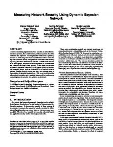
INTRODUCTION Understanding the pore pressure profile is crucial when drilling, so that the mudweight profile can be designed appropriately. This mud-weight forms a key part of any well plan. An example is shown in Figure 1. Generally, the mud-weight is designed to be slightly higher than the pore pressure. If the mud-weight is too low because the pore pressure has been poorly estimated, and a porous and permeable unit (e.g. a sandstone) is suddenly encountered, formation fluids may enter the wellbore (termed an influx) resulting in a kick, causing drilling problems and a well control incident. Conversely, if the mud-weight is too high, drilling mud can be lost to the porous unit, again causing well control problems. Predicting the pressure in sandstone before drilling (“pre-drill stage”) may be achieved by looking at data from sand layers in any neighbouring wells. However, as the tools used to 2
Mud-weight
Fracture Pressure Trend
Overburden Trend
Pore Pressure Trend
1.0 psi/ft
Bespoke overburden
Figure 1: Schematic depth/ppg plot illustrating the key components of a well plan i.e. pore pressure, fracture pressure and overburden or total vertical stress (TVS). Once these are defined, a mud-weight and casing design can be prepared (black lines). The fewer the casing strings required the more quickly/cheaply the well can be drilled. Uncertainty is highlighted on this figure by the double-headed arrows. In red is shown the overburden as generated by using a typically-applied 1.0 psi/ft gradient. This may be modified by using high quality, local density data, as shown by the bespoke overburden. This figure is from the Ikon GeoPressure training manual.
measure and record sandstone pressures rely on high permeability, understanding pressure in shale, where permeability is low, requires another approach. The standard shale pore pressure prediction workflow can be crudely summarised by the following steps.
1. Use the bulk density log (RHOB) to estimate the total vertical stress or overburden (Sv ) - in practice, resistivity, sonic and seismic velocity data can be used additionally. 3
2. Use the gamma ray (GR) and/or a combination of neutron porosity and RHOB to understand the lithology and so restrict the intervals for analysis to shales. 3. Generate a shale normal compaction trend (NCT) in terms of one of the logs, usually sonic transit time (∆T) or resistivity. This involves specifying matrix and sea-floor values for the log. 4. Use a published pore pressure prediction formula, such as Eaton (Eaton, 1975), Bowers (Bowers, 1995) or the Equivalent Depth Method (Foster and Whalen, 1966) to estimate vertical effective stress (VES, the difference between the pore pressure and the overburden). This uses only one log at a time, and relies on the normal compaction trend (or a slightly different curve for Bowers). 5. If pore pressure measurements are available that are believed to be in equilibrium with the shale, use these to calibrate the prediction, and repeat steps 3 to 5.
Existing work on uncertainty in pore pressure The procedure outlined above is deterministic, and as such it does not include a measure of uncertainty. Wessling et al. (2013) developed an algorithm to automate the pore pressure estimation process in such a way that uncertainties are accounted for. They focus on two parts of the process where human interaction is most at work: shale discrimination and the estimation of the NCT. For the NCT, they vary the depth interval considered normally compacted, and therefore over which the data are used, and fit an NCT to the data from every possible interval. Each NCT is then used for pore pressure prediction, creating a suite of pressure predictions that can be used to understand uncertainty. While Wessling et. al do account for uncertainty in the data, and in decisions over the depth at which overpressure begins, modern Bayesian statistical methods argue against automating out such 4
human interaction. Geoscientists will often have knowledge and experience that may not be reflected in the data. Furthermore, there will not always be sufficient log data at normally pressured depths, and in this situation the method of Wessling et al. (2013) will be unusable. Malinverno et al. (2004) and Moos et al. (2004) use Monte Carlo (MC) error propagation methods to asses parameter uncertainty for this workflow. For each input parameter (the sea floor and matrix log values for the NCT, the Eaton exponent, and so on) one must specify a probability distribution to reflect the uncertainty in that parameter. This may be derived from data, or a geoscientist may draw on their knowledge and experience to specify values. For example, for the matrix sonic transit time the user may choose a normal distribution with mean 110µs/ft and standard deviation 10µs/ft. Using these distributions a large number of random values is then generated for each input, producing many random ‘settings’ for the workflow. The workflow is then implemented at each of these settings, using some data, to generate a set of pore pressure predictions. The variation in these pore pressure predictions reflects the parameter uncertainty represented in the probability distributions. It is crucial to understand that the method we propose here goes far beyond MC error propagation. Our focus is on inference, as prediction is our primary aim. In our formulation, an understanding of error propogation is a quite trivial side-benefit, as shown in the sensitivity analysis we conduct. MC error propagation goes some way to understanding parameter uncertainty, but it ignores the uncertainty resulting from the workflow itself, which is arguably much more important. The equations used are simple, usually involving only a small number of variables and ignoring many sources of variation. MC error propagation assumes that the scientific model is perfect and that the only source of uncertainty is in the parameters used. MC methods are limited by the fact that they work with the existing method, which has some weaknesses that we will briefly explore. 5
The pore pressure system is such that each log may be affected by several properties of the system, and each property (e.g. lithology, pore fluid, pore pressure) is likely to influence several logs. It seems reasonable to collect all relevant logs and process them together to learn about these properties, rather than to treat them separately. Throughout the prediction process, geologists are able to draw on their extensive knowledge gained from experience with similar geological settings or with nearby fields. This is highly valuable information, yet there is no structure to include it. Either the geologist adjusts the predictions to better fit their expectations, or their input is ignored as the equations are used without changes. Neither of these approaches will produce the optimum outcome. Furthermore, the standard workflow as described is not a faithful representation of geologists’ understanding of the system. For example, it is commonly understood that the link between porosity and effective stress is key in understanding compaction, and that a wireline log is used as a proxy for the porosity. However, formulae such as Eaton’s relation (Eaton, 1975) relate effective stress (and therefore pore pressure) directly to the wireline log only, so that the effect of other data or parts of the system are either ignored, or accounted for in an ad hoc fashion. This makes for a model of the system that is less flexible, more difficult to interrogate, and more like a ‘black box’. To address these issues, we present a Bayesian network for pore pressure prediction. A Bayesian network allows us to model the system using our choice of scientific relationships, and to include uncertainty from various sources, including those relationships and their parameters. This method improves on a MC analysis, where the only uncertainty considered is observation error (or uncertainty about parameter values). Unlike MC, which is a method for analysing an existing model, a Bayesian network is a complete model in itself, built to best represent scientific understanding of the process; it is far from a ‘black box’.
6
Before proceeding, we should note that we are not suggesting that the underlying physics and chemistry of the processes involved are perfectly captured in the equations we have used. This is a matter for geoscientists to debate, not statisticians. However, the incorporation of uncertainty into those equations does provide for some slack in whether the equations represent an agreed underlying reality. The equations used within the statistical model may be updated as further geophysical research provides more insight into the underlying reality, but the basic statistical approach advised here would be unchanged. Indeed, the PP SDBN as presented in this paper is a preliminary model, including only fairly basic scientific relationships. However, the Bayesian principles underpinning it would remain the same as more complexity is added.
BAYESIAN NETWORKS The theory of Bayesian networks (Cowell et al., 1999; Jensen, 2007; Pearl, 1988) has led to many new applications of uncertainty modelling, in particular to complex problems where a large number of factors contribute to overall uncertainty. A clear and detailed explanation of Bayesian networks, with application to a geological example, is given by Martinelli et al. (2011). For further examples of Bayesian networks in a geoscience context, see Van Wees et al. (2008) and Martinelli et al. (2014). Bayesian networks derive from Bayesian statistical methodology, which is characterized by providing a formal framework for the combination of data with the judgements of experts such as reservoir engineers. A Bayesian network is simply a formal way of factorizing a multidimensional probability distribution over many variables into a product of simpler conditional distributions which represent dependencies more directly. This results in a mathematically equivalent, but more tractable, representation of the geophysical variables and their inter-
7
relationships. Unlike many Bayesian methods, Bayesian networks are not expressed in terms of prior distributions and likelihood functions; they are used to model systems where it is impossible or impractical to specify a prior or likelihood over all the parameters. We instead think in terms of smaller collections of parameters. Human expertise is expressed through: (1) defining the qualitative structure, i.e. the dependencies between variables; (2) defining how dependent variables behave given the values of other variables influencing them; and (3) describing how non-dependent variables behave in the problem at hand. See Zellner (1995) for a fuller comparison of Bayesian and traditional approaches, and Goldstein (2006) on the central importance of role (3) for uncertainty analysis in complex stochastic systems. In a dynamic Bayesian network (DBN) the same network structure is repeated to represent a system evolving. Usually this represents the passage of time, with the network repeated for each time step, but for us it will represent change in depth down a borehole. We conceal here some technical difficulties in working with DBNs, as they apply to all problems rather than just to pore-pressure estimation. These tend to be mathematical (not all probability distributions are easy to work with) and computational (the factorization for large stochastic systems is difficult). As DBNs become larger, computing with them becomes prohibitively expensive if standard methods are used. Therefore various authors have proposed schemes for working efficiently with large DBNs, for example Wilkinson and Yeung (2002) and Berzuini et al. (1997). Our needs are different, and so we develop a new approach, the sequential dynamic Bayesian network (SDBN). In an SDBN, the DBN is treated as a series of separate Bayesian networks, one for each step. When data are entered, the network is updated at the first step to produce posterior distributions. These are used to inform the nodes at the second step, through the links connecting the two steps, and the model is updated at the second step to produce posterior 8
distributions. These are fed to the third step, and so on. This means that the posterior distributions at each step reflect all data up to that point. This sequential updating makes the SDBN particularly appealing in situations where data are acquired sequentially, for example in real-time drilling.
A BAYESIAN NETWORK FOR PORE PRESSURE ESTIMATION The pore pressure system involves quantities of several different types. Some we may measure, such as wireline logs or drilling data. Others we cannot observe directly, such as shale pore pressure, effective stress or porosity. Some have a definite, measureable (at least in principle) physical meaning, whereas others are more conceptual. Although we do not know all their values, we have some understanding of the relationships between them, which we can represent in the structure of the Bayesian network. The pore pressure sequential dynamic Bayesian network (PP SDBN) works by modelling the system at each depth, with connections between depths to capture the relationships that act vertically. By ‘the system’ we mean the collection of quantities connected to pore pressure, and their interactions. Two consecutive depth levels of the PP SDBN are shown in Figure 2. Only the model’s more physical nodes are shown in Figure 2, for clarity. The formulae used in the probability distributions are formed from published information on geophysical relationships (Rider, 1996; Hearst et al., 2000; Hantschel and Kauerauf, 2009) and conversations with various individuals. Were an expert to find them inappropriate they could change the shapes of distributions or the values of model parameters. This might be the case especially if applying the model to a new location which is known to be different from the ‘average’ settings given here. In this sense the model is flexible. As with any model, flexibility is open 9
to abuse, with parameters being ‘fudged’ to give the best fit to data, but the emphasis here is on making judgements about properties of the system. Sensitivity analysis, which we will demonstrate in a later section, enables us to discover to which of the input parameters the PP SDBN output is most sensitive, and therefore which values we should put effort into learning about in order to reduce uncertainty. Since pore pressure is included as a node at each depth, it has a probability distribution which will be updated as data are entered. This gives us an estimate of pore pressure with uncertainty that accounts for each part of the model and all the data we have used. The same is true of any node, and so we also produce estimates (with uncertainty) of lithology, porosity, total vertical stress, matrix density and every other node included in the PP SDBN.
The model When describing edges connecting one depth to the next, we use superscripts to denote a variable at a specific depth. For example, Sv(zi ) is the total vertical stress at depth zi . For an offshore well, the PP SDBN requires an additional input, Psea , the pressure contributed by the seawater above the borehole, that sits outside the repeating part of the network shown in Figure 2. We model this using the known surface elevation depth and seawater density, which we model as normally distributed. The PP SDBN currently assumes an offshore context. Were it to be applied onshore, the model would need to be adapted to deal with the land mass above sea level, and also any ‘near surface’ issues. Given the vertical depth, we can form a probability distribution for the hydrostatic pressure (Phyd ) using the prior distribution we have specified for the hydrostatic gradient. This will reflect understanding of variations in fluid density due to salinity, temperature and any other factors. Where there is little knowledge of the area, it is possible to use global values to create a less informative prior, 10
11
Matrix density (ρma )
Porosity (φ)
Vertical effective stress (σv )
Matrix sonic (∆Tmat )
Sonic
Pore pressure (Pp )
GR
Depth zi−1
Acoustic factor (x)
Lithology
Excess PP parameter (λ∗ )
Hydrostatic pressure (Phyd )
Bulk density (ρb )
Fluid density
Total vertical stress (Sv )
Depth increment
Matrix density (ρma )
Porosity (φ)
Vertical effective stress (σv )
Matrix sonic (∆Tmat )
Sonic
Pore pressure (Pp )
GR
Depth zi
Acoustic factor (x)
Lithology
Excess PP parameter (λ∗ )
Hydrostatic pressure (Phyd )
Figure 2: A simplified version of the PP SDBN, showing how the system is modelled at each depth level. The connections between two levels are shown by dashed lines. Deterministic relationships are shown by dotted lines.
Bulk density (ρb )
Fluid density
Total vertical stress (Sv )
Depth increment
whereas an expert in the geology of the region should have more accurate knowledge, and would therefore choose a more restrictive prior distribution. In either case, the distribution for the hydrostatic gradient is likely to be narrow, since water density is well understood. At the first depth, the total vertical stress is formed using Psea and a normally distributed bulk density for the rock between the sea floor and the first depth covered by the data. For subsequent depths we use the depth increment and the total vertical stress and bulk density from the previous depth zi−1 . The bulk density data and posterior distribution for total vertical stress at zi are stored. They are then used to calculate the mean vertical stress at the next depth giving the normal distribution described by �
(zi−1 )
Sv(zi ) ∼ N Sv(zi−1 ) + (zi − zi−1 ) gρb
�
2 , σlith ,
(1)
2 represents uncertainty in the where g is the acceleration due to gravity. The variance σlith
calculation of Sv even with accurate bulk density data. Using the bulk density log to estimate Sv gives a more accurate estimate than having a prior distribution on the lithostatic gradient, as we are doing with the hydrostatic pressure. If bulk density data is unavailable then this part of the model still holds, but the bulk density node will pass on a probability distribution rather than a single value. If other wireline log data are available, then the distribution on bulk density will be updated to reflect them. The excess pore pressure parameter (λ∗ ) is a continuous value between 0 and 1, defined by λ∗ =
Pp − Phyd Sv − Phyd
(2)
as in Shi and Wang (1988), with Pp , Phyd and Sv as in Figure 2. We model λ∗ using a beta distribution. This is a standard way of handling a variable taking values in the interval [0, 1], allowing a variety of shapes. If λ∗ = 0 then there is no overpressure. If, hypothetically,
12
λ∗ = 1 then pore pressure is the same as the total vertical stress. In the PP SDBN there is an edge from λ∗ at one depth to λ∗ at the next, indicating that the prior distribution for one layer comes from the posterior distribution for the previous layer. We also inflate slightly the prior variance for λ∗ for the next layer in order to avoid λ∗ converging to a single point, or expressing over-confidence. Because of this dynamic link, the excess pore pressure parameter is expected to remain the same from one depth to the next, this equates to a slight increase in pore pressure. Although small changes in λ∗ are favoured in the conditional distributions we choose, we ensure that more dramatic jumps are still possible. The nodes Sv , Phyd , λ∗ and pore pressure (Pp ) are linked deterministically, through the equation (3)
Pp = Phyd + λ∗ (Sv − Phyd ) .
When data are entered into the model these nodes’ distributions will be constrained by information coming from the depth, which mostly constrains Sv and Phyd , and by VES, which will have been constrained by porosity through information from the wireline logs. The posterior distribution of λ∗ from the previous depth will influence the current λ∗ , and this too will influence the pore pressure posterior distribution. The link between porosity (φ) and VES is the most important part of the model. Figure 2 shows lithology and VES as parents of porosity, however this is a simplification. This part of the model is shown in more detail in Figure 3. The conditional distribution for porosity is �
h
i
�
φ | σv , φmin , φml , kφ , σφ2 ∼ N φmin + (φml − φmin ) exp −10−6 kφ σv , σφ2 ,
(4)
based on equations found in Hantschel and Kauerauf (2009). The parameters φmin , φml , kφ and σφ2 each depend on the lithology. Again, the actual form of the relationship between porosity, VES and lithology can be changed as required.
13
Vertical effective stress (σv )
Minimum porosity (φmin )
Lithology Mudline porosity (φml ) Porosity exponent (kφ )
Porosity variance � � σφ2
Porosity (φ)
Figure 3: A close-up on the part of the PP SDBN modelling compaction.
By using this model, the PP SDBN reflects the fact that different lithologies compact differently. For any lithology and VES value, there is a probability distribution for porosity as shown in Figure 4. 0.8
Porosity
0.6 lith Shale
0.4
Sandstone 0.2
0.0 0
20
40
60
VES (MPa)
Figure 4: The compaction curves in the model. The mean (in a solid line) and central 50% and 95% intervals (shown by shading) are given to show the spread of the probability distribution of porosity for each value of vertical effective stress and lithology.
A key feature of the distribution shown in Figure 4 is that porosity is more uncertain in sandstones than in shales, since shale compaction is generally better understood. This greater uncertainty feeds through the model, and so where the posterior distribution for lithology favours shale, the posterior distribution for pore pressure will be narrower than in what the 14
model estimates to be sandstones. The logic of the model is similar to that of the equivalent depth method for estimating pore pressure; it is assumed that, under the same lithological conditions, a particular value of VES will lead to a particular value of porosity. Since we know the depth, and therefore have an estimate for Sv , we can use this to estimate pore pressure. The PP SDBN presented here is therefore based on mechanical compaction. The lithology posterior distribution will take the form of probabilities of sandstone and shale. For example, in the posterior distribution samples for depth zi−1 , 10% might be sandstone with the remaining 90% being shale. Therefore in the posterior distribution at depth zi−1 (z
)
the probability of the lithology being shale is pshi−1 = 0.9. The sequential model includes a lithology transition matrix
psst|sst
psh|sst
psst|sh psh|sh
,
which gives the probability of each lithology at depth zi given the lithology at depth zi−1 , (z )
(z )
and this, together with the posterior samples from zi−1 , is used to generate pshi and pssti . Gamma ray (GR) count is strongly influenced by lithology, so in the PP SDBN the GR variable is represented as a child of lithology. We must therefore define a conditional probability distribution for GR for each kind of lithology considered, as we expect the GR log to behave differently for different lithologies. In the PP SDBN we use the Gamma ray index (IGR ) so that this variable is standardised to between 0 and 1. In practice, GR is observed via wireline log data. Hence, using Bayes Theorem, we can make inferences about unobserved lithology, and any other nodes connected to lithology such as porosity, from the observed GR wireline log. Bulk density (ρb ) is another node in Figure 2 that can often be constrained by observed data.
15
The key equation in understanding its surrounding links is (5)
ρb = φρf l + (1 − φ) ρma ,
where ρf l and ρma are fluid and matrix density respectively and φ is porosity. The matrix density depends on the lithology (specifically on the dominant mineral composition), and the fluid density on the pore fluid type. Figure 5a shows the default probability distribution for matrix density for sandstone and shale. One could argue that there is too much overlap between the two, however this ensures that the model does not ‘get stuck’ in a particular
Probability density
Probability density
lithology. Figure 5b shows some examples of alternative distributions for shale matrix density.
Shale Sandstone
2600
2700
Matrix density (kgm−3)
2800
2600
(a)
2700
Matrix density of shale (kg m3)
2800
(b)
Figure 5: Examples of possible prior distributions for matrix density (ρma ). (a) Current probability distribution for matrix density (ρma ) for sandstone and shale. (b) Possible alternative distributions for matrix density for shale. For example, lower values for a smectite rich formation and higher values for illite rich shale.
At present, the pore fluid type node has no parents, and it is assumed that the rock is predominantly water-filled.
16
We base the conditional distributions for sonic transit time (∆T) on the equation
∆T =
∆Tmat , (1 − φ)x
(6)
where ∆Tmat is the matrix sonic transit time and x is an acoustic formation factor. This relationship is presented by Raymer et al. (1980) for sandstones and by Issler (1992) for shales. The distributions for ∆Tmat and x depend on lithology, and ∆T is then normally distributed with Equation (6) used as the mean. Equation (6) was developed from deep borehole data which do not include shallow depths, typically less than 500m below sea-bed, and our model has not been applied to shallow depths on account of absence of data in the example wells. One could instead use Wyllie’s time average equation (Wyllie et al., 1956), in which case a fluid sonic transit time node would be introduced and the acoustic formation factor x removed. However, both Raymer et al. (1980) and Issler (1992) propose the form in Equation 6 as an improvement, stating that it better captures the curvi-linear relationship between porosity and ∆T, and is less prone to producing unrealistic porosity values, or requiring extensive tuning. The PP SDBN was implemented in R (R Development Core Team, 2011), with links to JAGS (‘Just Another Gibbs Sampler’). JAGS is a Gibbs sampling software, which we use to evaluate the posterior distributions of the nodes in the Bayesian network. Rather than find the posterior distributions analytically, the Gibbs sampler generates samples of values from each posterior distribution, which can then be used to understand the distribution. This is a standard way of approaching Bayesian networks (Bernado and Smith, 1994). A simplified example of how the Gibbs Sampler works is provided in the supplementary materials.
17
Advantages of this method Unlike traditional methods, the PP SDBN models the interactions between different quantities in the system. For example, we learn about the lithology using the GR, sonic and bulk density logs simultaneously, and the posterior probability distribution for porosity reflects both the bulk density and sonic. Therefore the uncertainty reflects the extent to which different sources of information agree with one another. Because the PP SDBN will learn from whatever set of information it is given, it is not dependent on any particular set of log data being available. If part of a log is missing for some depth range, that node’s conditional distribution will be used to learn about its behaviour in light of all available data. Therefore this method is flexible and robust, not requiring a particular log or combination of data to be available at all depths, unlike MC error propagation, which is not robust to missing data. As the PP SDBN is a full probabilistic model of the system, we learn about not just pore pressure but all unobserved nodes through their posterior distributions. This allows us to more fully assess our model, and also to learn more about the system. This is partially the case when using MC with standard pore pressure estimation; for example, we will generate a sample of lithologies having perturbed the shale cut-off value, or we may have a sample of total vertical stress values by perturbing parameters relating to the estimation. In contrast though, these samples will reflect only the small set of data types involved in that part of the process, whereas when using a Bayesian network the posterior distribution reflects all the data that have been used for the model. This reveals the fundamental difference between MC error propagation and the PP SDBN. The former can only assess uncertainty in an existing model whereas the latter incorporates a fully joint model of the entire system. There is an equivalence in the results produced by the SDBN approach and MC error propagation, in the sense that if we applied an idealised error propagation approach to our model, the results of the error propagation would be exactly the same as the prediction uncertainties 18
produced by our model. If we regard the PP SDBN as a gold standard approach combining the best available synthesis of data and human expertise, we could in principle examine any discrepancies between it and uncertainties produced by MC error propagation applied to other modelling approaches. However, this would need substantial effort to match input choices and would in any case only allow us to conclude that different models can produce different answers. In the SDBN, expert knowledge and data are combined in a rigorous way using Bayes Theorem. As with any other method developed for pore-pressure prediction, the quality of the results depends on the quality of judgements about model relationships and so forth, but with the advantage for the SDBN approach that we formally quantify the expert’s uncertainty in the model via probability distributions. The expert’s uncertainty is therefore reflected in the final pore pressure estimate. As pointed out earlier, the structure of the model is also subjective and so should be designed with care (Plummer, 2014; Su and Yajima, 2014). Note however that the traditional workflow and the corresponding “standard” methods chosen are themselves highly subjective, but not handled within the rigorous formal statistical framework of a Bayesian network.
EXAMPLES
West Africa 1 Figure 6 shows data from a well in West Africa, with predictions made by the PP SDBN.
19
2500
2500
2500
2500
2500
4000
3500
4000
4500 0.5
IGR
1.0
3500
4000
4500 0.0
2.75
Bulk density (gcc)
3500
3500
● ● ●
4500
4500 200
● ●
4000
4000
4500 2.25
3000
3000
TVD ml (m)
3500
3000
TVD ml (m)
3000
TVD ml (m)
3000
TVD ml (m)
True Vertical Depth below mudline (TVD ml) (m)
●
400
40
Sonic (us/m)
Lithology
60
80
100
Pressure (MPa)
Figure 6: West Africa 1 (From left to right) 1. Gamma ray index data; 2. Bulk density data; 3. Sonic transit time data; 4. Lithology estimated by SDBN (blue is shale, orange is sandstone); 5. Pore-pressure estimated by SDBN, with mean and central 50% and 95% intervals shown by shading. Mean and central 95% are shown for total vertical stress and hydrostatic pressure, although there is little uncertainty in these compared to pore pressure and so they appear as lines. Sandstone pore pressure data is shown by red dots in the pressure plot. Note that these pressure observations are not used as input data to the PP SDBN.
This interval was chosen because it appeared to be predominantly shale but contains several sandstone intervals in which pore pressure was measured. Of the six sandstone pressure measurements, the shallowest and the deepest three are judged by experts to be in isolated sandstones, and therefore our shale pore pressure estimate should match them. As they are taken from sandstones, we can use their depths to assess the performance of the lithology estimation, and indeed they are all matched by regions of sandstone in the lithology plot. The two pressure measurements around 3350m are thought to be in a thicker and more laterally extensive sandstone that is slightly drained, and the lithology posterior distribution indeed suggests a thicker layer of sandstone here. The estimated pore pressure trajectory above this is in agreement with our experts’ expectations. The sharp spikes around 3800m coincide with 20
a casing point, which has been identified as a sandstone by the SDBN as this knowledge is outside its scope. However, it has not influenced the nearby results, showing that the SDBN is robust to unexpected results. Figure 7 shows the samples from the posterior distributions of pore pressure and porosity at three particular depths. Such plots can be made for any unobserved node, at any depth, and so can be useful for developing a greater understanding of uncertainty. 2800m (TVDml)
3200m (TVDml)
3800m (TVDml)
0.075 0.050 0.025 0.000
Probability Density
Probability Density
Probability Density
0.100 0.15
0.10
0.05
0.00 30
40
50
60
70
80
0.15
0.10
0.05
0.00 30
Pore pressure (MPa)
40
50
60
70
80
30
Pore pressure (MPa)
40
50
60
70
80
Pore pressure (MPa)
(a) Pore pressure posterior distributions. 3200m (TVDml)
40
20
10
0
3800m (TVDml) 40
Probability Density
30
Probability Density
Probability Density
2800m (TVDml)
30
20
10
0 0.00
0.25
Porosity
0.50
30 20 10 0
0.00
0.25
0.50
0.00
Porosity
0.25
0.50
Porosity
(b) Porosity posterior distributions. Figure 7: Posterior distributions at three depths (all shale) in West Africa 1.
Figure 8 compares the posterior pore pressure distribution for West Africa-1 for different combinations of input data. This demonstrates the reduction in uncertainty that can come with including additional data. Without the control from the gamma log the lithology is poorly constrained leading to a significantly worse pressure estimation. 21
2500
2500
2500
●
●
● ●
3500
● ● ●
4000
3000
TVDml (m)
3000
TVDml (m)
TVDml (m)
3000
●
● ●
3500
● ● ●
4000
4500 60
80
100
● ● ●
4500 40
Pressure (MPa)
(a) IGR , RHOB and DT.
3500
4000
4500 40
● ●
60
80
100
Pressure (MPa)
(b) IGR and RHOB only.
40
60
80
100
Pressure (MPa)
(c) RHOB only.
Figure 8: Comparing the results of the SDBN with different datasets: (a) using all available logs; (b) using gamma and density only, though the general shape of the curve is the same the level of uncertainty has increased; (c) density only.
SENSITIVITY ANALYSIS The PP SDBN is a statistical model constructed from expressed geophysical relationships and tuning parameters. The default values we supply can be used for the tuning parameters, or a reservoir engineer may supply more carefully considered inputs, depending on their expertise and local knowledge. The PP SDBN lends itself well to sensitivity analysis techniques. The aim of sensitivity analysis is to discover how variation in the output can be explained by variation in the collection of inputs. Variation in inputs can be attributed to several sources. 22
A physical quantity may be subject to measurement error, or there may be a high level of uncertainty about a particular parameter owing to a lack of information or understanding of the system. Sensitivity analysis reveals how this uncertainty propagates to the output, and therefore indicates the degree of confidence we can have in the model’s results. For example, if a model’s output is highly sensitive to a physical parameter about which little is known, there is consequential uncertainty surrounding the model output. Sensitivity analysis allows us to more deeply examine how the model is working, and whether it resembles the real system in the way that we expect. For example, system experts are likely to expect some parameters to be among the most influential. If the sensitivity analysis shows them to be insignificant in the model, this suggests that the model is not representing the system as intended. Learning which are the most crucial parameters for tuning the model can help improve predictions. If current estimates for the values of these parameters are not sufficiently precise to give confidence in the output values, further research should be conducted into these parameters. Equally, the model can also be simplified by eliminating variables to which the model is not at all sensitive. Saltelli et al. (2000) give a thorough account of the theory and techniques of sensitivity analysis .
Preliminary examples Here we demonstrate some simple preliminary techniques, before going on to demonstrate a more comprehensive method. To gain some insight into how influential a parameter is, one can hold all others fixed at their default value, then vary the parameter in question. In the following examples we do this for West Africa 1, and with each parameter being varied between 3 values: low, default and high. The specific values for each parameter were formed by surveying geologist colleagues. This was not a thorough elicitation, but a casual experiment. Nevertheless, the ranges provided should give reasonable results. 23
Figure 9 compares posterior probability distributions for pore pressure when three different input parameters are varied. This could be done for any other unobserved node, for example porosity or total vertical stress. The leftmost plot, in which an input (the first scale parameter of a beta distribution) relating to sea-floor porosity in shales has been varied, shows that this parameter has little effect on pore pressure at this depth for this well. The three posterior distributions are very similar. The middle plot, in which the mean matrix sonic transit time of shale (in sm−1 ) is varied, shows a stronger influence.
0.100
0.075
0.050
0.025
0.000
0.075
Probability density
Probability density
Probability density
0.100
0.050
0.025
0.000 30
35
40
45
Sea−floor porosity parameter 1 (shale)
(a)
11.16
20.91
35
40
45
50
55
Pore pressure (MPa) 30.66
0.2
0.1
0.0 30
Pore pressure (MPa)
0.3
Mean matrix sonic (shale)
2e−04
(b)
3e−04
30
40
50
60
Pore pressure (MPa) 4e−04
Matrix sonic SD
2e−06
6e−06
1e−05
(c)
Figure 9: Posterior probability distributions for pore pressure at 2600m. In each plot, all but one of the input parameters have been held at its default value, and one has been varied, as shown in the legend beneath each plot. The mean for each posterior distribution is also shown by a vertical line in the corresponding colour. (a) Sea-floor porosity parameter 1 for shale. This is the first shape parameter of a beta distribution. (b) Mean matrix sonic for shale, in s/m. (c) Standard deviation of matrix sonic, in s/m.
The three posterior distributions are clearly separated, and the means differ by around 8MPa. Therefore better understanding the matrix sonic transit time in shale would increase our confidence in pore pressure. The third plot, in which the standard deviation (SD) of the matrix sonic transit time is varied, shows different behaviour still. It appears that for some value of matrix sonic SD between the low and default values, there is a discrete change in model behaviour. Studying the posterior distributions shows that this relates to lithology; the 24
posterior samples for the default and high values contain much more sandstone than those from the low value, and this difference has manifested itself in the pore pressure posterior distributions. Figure 10 summarises the results of performing this analysis on several input parameters, by plotting the means of the posterior distributions for each parameter that has been varied, in order of range. 2600m
3700m
Matrix sonic SD
|
Matrix sonic SD
|
Mean matrix sonic (shale)
|
Mean matrix sonic (shale)
|
Matrix density SD (sandstone)
|
Matrix density SD (sandstone)
|
Porosity variation factor (shale)
|
Sea−floor porosity parameter 1 (shale)
|
Sea−floor porosity parameter 1 (shale)
|
Porosity variation factor (shale)
|
Mean matrix density (shale)
|
Mean matrix density (shale)
|
40
50
60
Mean pore pressure (MPa)
70
80
Mean pore pressure (MPa)
Figure 10: Tornado plots (Howard, 1988) for some SDBN input parameters, at two depths in West Africa 1. The left pointing arrows mark the mean posterior pore pressure for the lower of the three input values, the right pointing arrows for the upper value and the vertical bar for the default. Outward pointing arrows (for example as with matrix density SD) imply a positive correlation between that input and the mean pore pressure. Inward pointing arrows (as with matrix sonic SD) imply a negative effect.
Morris screening design To gain insight into which are the more influential parameters, we will use a one-at-a-time screening design proposed by Morris (1991). Once complete, we have a number of elementary effects values for each input parameter. Each one can be thought of as an estimate of the effect of changing that input from its minimum to its maximum, with every other input held the same, somewhat like a partial derivative of the output with respect to that input 25
parameter. Therefore a large (negative or positive) elementary effect suggests an influential parameter. One close to zero suggests a more negligible parameter. In summary, the following obserservations can be made:
• If the elementary effects for input i have a mean close to zero and a low variance, input i appears to have little effect; • If the elementary effects for input i have a high (in magnitude) mean and a low variance, input i appears to have a strong linear effect; • If the elementary effects for input i have a high variance, input i appears to be involved in interactions with other inputs, or to have a non-linear effect.
Example: West Africa 1 In the PP SDBN there are 38 input parameters, each of which we chose initially to vary. We choose five values for each input paramter, and run the model 1000 times in total. We stipulated that we must produce at least 20 elementary effects for each input parameter. Figure 11 shows the elementary effects for two depths in West Africa 1. The first depth (2670m) is near to the top of the interval in which the experiment was run. Above this point, the borehole is almost entirely shale, and this is true in almost all of the input space. By 2770m (the depth of the second plot), there has been some sandstone, with the PP SDBN estimating more sandstone at some input value settings than at others. This could account for the higher variability elementary effects at the deeper point.
26
Mean Pp, 2770m
● ●● ●
●
● ● ● ● ●●● ● ●● ●
●
● ●
● ● ● ●
input
input
Mean Pp, 2670m porsd_sh_fac b_porml_sh b_pormin_sh porsd_sh_add rhoma_sh_sd acfac.sd rhoma_sst_sd rhoma_sh_mean a_pormin_sst a_kpor_sh dtma_mean_sst rho_gas_sd p_sh_sh b_pormin_sst rho_water_sd a_porml_sst rho_water_mean rhoma_sst_mean porsd_sst_add aigrsh rho_gas_mean a_swater b_kpor_sst acfac_mean_sst a_kpor_sst acfac_mean_sh dtma.sd p_sh_sst p_shale pdrain_sst a_pormin_sh a_porml_sh b_porml_sst porsd_sst_fac b_kpor_sh bigrsst dt.sd dtma_mean_sh
● ● ●
● ● ● ● ● ●
● ● ● ● ●
● ● ● ●
●
● ● ●
−20
−10
0
10
porsd_sh_fac b_porml_sh b_pormin_sh rhoma_sst_sd p_shale pdrain_sst a_kpor_sst a_swater porsd_sh_add dt.sd rhoma_sh_mean a_kpor_sh dtma.sd p_sh_sst acfac_mean_sst a_pormin_sst rhoma_sst_mean bigrsst rho_gas_sd b_kpor_sst rho_water_sd b_pormin_sst a_porml_sst rho_water_mean a_porml_sh p_sh_sh porsd_sst_add aigrsh rhoma_sh_sd porsd_sst_fac b_porml_sst rho_gas_mean acfac.sd dtma_mean_sst a_pormin_sh b_kpor_sh acfac_mean_sh dtma_mean_sh
20
●●● ●
●
●
●
●●●
● ●●●
●
● ● ●
●
●
●
● ●● ● ●
●
●
● ●
● ● ●
● ●
● ●
●
● ●
● ●
●
●
●
● ● ●
● ●
●
●
●
● ● ● ●●●
●
● ●
●
●●
●● ● ●●
●
● ●● ●
●
●
●
●● ●
●
●
●●
●
●
● ● ●
●
●
● ●
●●
●
●
●
● ●● ●
●
●
●
● ●
−20
Elementary effect (MPa)
●
●●
−10
●
0
10
20
Elementary effect (MPa)
Figure 11: Elementary effects for mean pore pressure at two depths in West Africa 1, ordered by median elementary effect. Points falling outside the interquartile range (IQR) by more than 1.5×IQR will be plotted as outliers.
The most influential parameters remain the same in each plot, with ‘dtma_mean_sh’ (mean matrix sonic transit time in shale) having a negative effect on mean pore pressure, and ‘porsd_sh_fac’ (σφf ac ) having a positive effects. The distributions of these elementary effects are similar in each plot. ‘b_porml_sh’ and ‘b_pormin_sh’ (these are shape parameters for the mudline porosity and minimum porosity respectively in shales) have a slight positive effect in each case. Otherwise, the elementary effects are centred around zero, some with little spread. Therefore our primary focus would be on the four parameters already mentioned, and it may well be possible to eliminate some of the consistently negligible input parameters without degrading the result of the pore pressure prediction.
27
DISCUSSION The problem we have addressed in this paper is that of quantifying uncertainty in pore pressure predictions in a meaningful way. We have approached this problem from an entirely fresh perspective, based on a rigorous formal statistical method and present a proof-of-concept model that is highly adaptable. The appropriate mathematical machinery is the Bayesian network, which allows us to express causal dependencies between the geophysical elements which make up our understanding of the relationships between pressures, lithology, porosity, wireline logs, and so forth. This kind of approach is open and transparent, with all the ingredients (structure, experiential judgements, data) having a clear role and implication. The Bayesian network allows us to collect together expert knowledge, uncertainty and data into a rigorous and coherent model, so that the resulting pore pressure probability distribution makes sense of these. Through sensitivity analysis we can understand which of the input parameters are the most influential. This can lead to an increased focus in these areas, and therefore to a reduction in uncertainty in pore pressure as they are better understood. The PP SDBN is a flexible core framework that can be extended in many ways to represent the pore pressure system and to be useful practically in the process of planning and drilling a well. From a geological perspective, log data and seismic data are inherently less reliable for pressure understanding than direct pressure measurements, thus any technique that can be developed that helps the geologist visualise, understand and therefore reduce the uncertainty in these data types is highly valuable and will result in more accurate pressure prediction. Moreover, if the same approach can also define and quantify prior understanding of how a system behaves, and express uncertainty about this understanding, then the final pressure profile will be much more robust.
28
Geological basins are complex environments, where multiple factors affect a simple variable such as porosity. Porosity (or often a proxy variable such as sonic transit time or bulk density) is used directly to relate to pore pressure and yet many co-dependant factors influence its value. The PP SDBN allows us to jointly model these factors, their co-dependence and our uncertainty. This provides a more holistic way to approach, in this example, porosity. The effects of data gaps or missing logs can be quickly assessed in terms of our ability to define an accurate porosity and subsequently, pressure. Expert knowledge and data are combined in this approach so that it is geologically based. Uncertainty in the expert judgements is captured in the conditional probability distributions, and is reflected in the posterior probability distributions attached to the pressure estimates. The PP SDBN as presented in this paper is a preliminary proof-of-concept model, involving a limited selection of data types and assuming disequilibrium compaction as the pressure generating mechanism. However, the Bayesian network structure lends itself to augmentation. To develop the PP SDBN, more data types would need to be incorporated. This includes additional log measurements, such as resistivity and neutron density. The caliper log could also be introduced in order to inform the uncertainty based on the borehole quality. By learning from the equivalent circulating and static densities, along with any connection gas or kicks, we could put logical constraints on the pore pressure. An extension to the PP SDBN proposed here for pre-drill pressure prediction would be the incorporation of velocity information from surface seismic reflection data. As part of the seismic processing work-flow, several velocity models can be derived ranging from simple normal-moveout to tomographic inversion and more recently to full-wave inversion. The choice of which to use depends on the complexity of the problem (Cibin et al., 2004). Velocity models and their relationship to pore pressure can be further refined by calibration to offset wells, if available (Den Boer et al., 2006; Sayers et al., 2006). To ensure consistency with the SDBN’s modelling of uncertainty, the chosen velocity model should also include 29
an estimate of its own uncertainty, ideally computed in a compatible Bayesian manner, as for example by Caiado et al. (2012). The uncertainty in the velocity model would then be reflected in the pre-drill pore pressure distribution. Incorporating this surface derived velocity information into the PP SDBN would be effected by addition of a node as an alternative for or to complement the wireline log nodes. A desirable development would be to extend the SDBN to three dimensions to create a full 3D probabilistic pore pressure estimate, as for example in Doyen et al. (2003). There are two key challenges here. Firstly, the SDBN is a computationally intensive method, and extending to 3D would multiply this problem. Secondly, extending to 3D would require us to carefully think about horizontal correlation, and how to capture features such as lateral transfer and drainage, extensional and compressional stress and anisotropy. It is worth noting that Doyen et al. (2003) avoid this issue by deriving their probability distributions empirically from well data: their worked example uses data from 21 nearby wells. The first issue may be overcome by use of a large multi-core computer, or by use of a velocity model such as that from Caiado et al. (2012), which could be used to reduce the size of the dataset. The second requires more thought. It is difficult to validate the approach of Doyen et al. (2003) inasmuch as linking the empirically derived parameters to physical realities. Our preferred approach would be to model these parameters, in which case the physical model, the data and judgements used to populate it, and the inferences and predictions drawn from it, are transparent and open to scrutiny.
CONCLUSION In this paper we have presented the PP SDBN, a novel, statistically rigorous framework for quantifying uncertainty in pore pressure estimation. The Bayesian network we have developed
30
allows the geologist to capture their scientific understanding of the pore pressure system, in order for this to be updated in light of any available data. The PP SDBN as we have presented it is currently applicable to those basins where mechanical compaction is the generator of pore pressure. The flexible nature of the network means that adapting it to account for more data types in the future (e.g. pre-drill seismic velocity models, or real time data), or a more complicated scientific model (e.g. including chemical compaction, or non-vertical stresses) is feasible. The PP SDBN is an improvement on methods such as Monte Carlo; the pore pressure uncertainty will not necessarily be smaller, but it has a clear meaning, having arisen from a careful specification of the expert’s understanding of the system. The uncertainty reflects the data and expert knowledge in a way that is not possible with Monte Carlo, since the PP SDBN is a fully probabilistic model of the system. The accuracy of the PP SDBN’s pore pressure prediction (the mean of the posterior distribution) will depend on the geophysical relationships used, but because posterior distributions (and hence predictions) are produced for all nodes, the model can be interrogated and understood in terms of how it models each part of the system, rather than pore pressure alone. Previous approaches to quantifying uncertainty tend to be ad hoc; industry-standard relationships such as Eaton or the equivalent depth method do not easily allow all sources of uncertainty to be easily represented. Pressure is calculated on an increasing depth basis, ignoring the co-dependency of many of the variables in these algorithms. Our method differs in that it offers a coherent structure for containing the data, geological knowledge and physical understanding available, with assessments of uncertainty on each of these elements. The conditional probability distributions are specified to best represent our understanding of how the quantities in the system interact. Because of this, the method is transparent, in that uncertainty in the posterior pore pressure distribution can be understood in terms of uncertainty in the input parameters and scientific relationships used in the PP SDBN. It is 31
therefore a more effective tool for capturing and displaying uncertainty, and for indicating deficiencies in understanding, as we have shown through sensitivity analysis. As with any decision-support tool, the quality of the prediction depends on the quality of the model, but also overtly here on the quality of the human expertise supplied to it. Pore pressure prediction is inherently uncertain, especially in shale lithologies where the low permeability precludes the use of direct pressure tests. Many assumptions have to be made, and it is typically problematic to test which of these assumptions are the most reliable, and which particular parameter holds the most weight. The PP SDBN allows careful and rigorous analysis of these factors, resulting in a clearer understanding of the geological system in terms of its influence on the pressure regime. This leads to more accurate pressure prediction and ultimately to the more cost-effective and safe drilling of future wells.
Acknowledgements With thanks to the sponsors of the GeoPOP3 project, BG, BP, Chevron, ConocoPhillips, DONG Energy, E.ON, Eni, Petrobras, Petronas, Statoil, Total and Tullow Oil, for financial support, and also to GeoPOP3 colleagues for their advice and support.
References Bernado, J. M., and A. F. Smith, 1994, Bayesian theory: Wiley. Berzuini, C., N. G. Best, W. R. Gilks, and C. Larizza, 1997, Dynamic conditional independence models and markov chain monte carlo methods: Journal of the American Statistical Association, 92, 1403 – 1412.
32
Bowers, G., 1995, Pore pressure estimation from velocity data - accounting for overpressure mechanisms besides undercompaction: SPE drilling & completion, 10, 89–95. Caiado, C. C., R. W. Hobbs, and M. Goldstein, 2012, Bayesian strategies to asses uncertainty in velocity models: Bayesian Analysis, 7, 211–234. Cibin, P., M. D. Martera, M. Buia, D. Calcagni, D. J. Runcer, and T. Talkan, 2004, What seismic velocity field for pore pressure prediction?, in SEG Technical Program Expanded Abstracts 2004: Society of Exploration Geophysicists, 1531–1534. Cowell, R., A. Dawid, S. Lauritzen, and D. Spiegelhalter, 1999, Probabilistic networks and expert systems: Springer. Den Boer, L. D., C. M. Sayers, Z. R. Nagy, P. J. Hooyman, and M. J. Woodward, 2006, Pore pressure prediction using well-conditioned seismic velocities: first break, 24, 43–49. Doyen, P., A. Malinverno, R. Prioul, P. Hooyman, S. Noeth, L. den Boer, D. Psaila, C. Sayers, T. Smit, C. van Eden, et al., 2003, Seismic pore pressure prediction with uncertainty using a probabilistic mechanical earth model, in SEG Technical Program Expanded Abstracts 2003: Society of Exploration Geophysicists, 1366–1369. Eaton, B. A., 1975, The equation for geopressure prediction from well logs: Presented at the Fall Meeting of the Society of Petroleum Engineers of AIME, Society of Petroleum Engineers. Foster, J., and H. Whalen, 1966, Estimation of formation pressures from electrical surveys offshore Louisiana: Electrical Logging, 165 – 171. Goldstein, M., 2006, Subjective bayesian analysis: Principles and practice (with discussion): Bayesian Analysis, 13, 403–420. Hantschel, T., and A. I. Kauerauf, 2009, Fundamentals of basin and petroleum systems modeling: Springer. Hearst, J. R., P. H. Nelson, and F. L. Paillett, 2000, Well logging for physical properties: Wiley. Howard, R. A., 1988, Decision analysis: practice and promise: Management Science, 34, 33
679–695. Issler, D., 1992, A new approach to shale compaction and stratigraphic restoration, BeaufortMackenzie Basin and Mackenzie Corridor, Northern Canada: The American Association of Petroleum Geologists Bulletin, 76, 1170 – 1189. Jensen, F., 2007, Bayesian networks and decision graphs: Springer. Malinverno, A., C. M. Sayers, M. J. Woodward, R. C. Bartman, et al., 2004, Integrating diverse measurements to predict pore pressure with uncertainties while drilling: Presented at the SPE Annual Technical Conference and Exhibition, Society of Petroleum Engineers. Martinelli, G., J. Eidsvik, R. Hauge, and M. D. Forland, 2011, Bayesian networks for prospect analysis in the north sea: AAPG bulletin, 95, 1423–1442. Martinelli, G., J. Eidsvik, K. Hokstad, R. Hauge, et al., 2014, Strategies for petroleum exploration on the basis of bayesian networks: A case study: SPE Journal, 19, 564–575. Moos, D., P. Peska, C. Ward, A. Brehm, et al., 2004, Quantitative risk assessment applied to pre-drill pore pressure, sealing potential, and mud window predictions from seismic data: Presented at the Gulf Rocks 2004, the 6th North America Rock Mechanics Symposium (NARMS), American Rock Mechanics Association. Morris, M. D., 1991, Factorial sampling plans for preliminary computational experiments: Technometrics, 33, pp. 161–174. Pearl, J., 1988, Probabilistic reasoning in intelligent systems: networks of plausible inference: Morgan Kaufmann. Plummer, M., 2014, rjags: Bayesian graphical models using mcmc. (R package version 3-13). R Development Core Team, 2011, R: A language and environment for statistical computing. R Foundation for Statistical Computing, Vienna, Austria. (ISBN 3-900051-07-0). Raymer, L., E. Hunt, and J. Gardner, 1980, An improved sonic transit time-to-porosity transform: Presented at the SPWLA 21th Annual Logging Symposium. Rider, M., 1996, The geological interpretation of well logs, second ed.: Whittles. Saltelli, A., K. Chan, and E. Scott, 2000, Sensitivity analysis: Wiley. 34
Sayers, C. M., L. D. den Boer, Z. R. Nagy, and P. J. Hooyman, 2006, Well-constrained seismic estimation of pore pressure with uncertainty: The Leading Edge, 25, 1524–1526. Shi, Y., and C.-Y. Wang, 1988, Generation of high pore pressures in accretionary prisms: Inferences from the Barbados subduction complex: Journal of Geophysical Research, 93, 8893 – 8910. Su, Y.-S., and M. Yajima, 2014, R2jags: A package for running jags from r. (R package version 0.04-01). Van Wees, J.-D., H. Mijnlieff, J. Lutgert, J. Breunese, C. Bos, P. Rosenkranz, and F. Neele, 2008, A bayesian belief network approach for assessing the impact of exploration prospect interdependency: An application to predict gas discoveries in the netherlands: AAPG bulletin, 92, 1315–1336. Wessling, S., A. Bartetzko, and P. Tesch, 2013, Quantification of uncertainty in a multistage/multiparameter modeling workflow: pore pressure from geophysical well logs: Geophysics, 78, 101–112. Wilkinson, D. J., and S. K. Yeung, 2002, Conditional simulation from highly structured gaussian systems, with application to blocking-mcmc for the bayesian analysis of very large linear models: Statistics and Computing, 12, 287–300. Wyllie, M., A. Gregory, and L. Gardner, 1956, Elastic wave velocities in heterogeneous and porous media: Geophysics, 21, 41–70. Zellner, A., 1995, Bayesian and non-bayesian approaches to statistical inference and decisionmaking: J. Computational and Applied Mathematics, 64, 3–10.
35