A shape based, viewpoint invariant local descriptor

A shape based, viewpoint invariant local descriptor Mihai Osian1 , Tinne Tuytelaars1 , and Luc Van Gool1,2 1

Katholieke Universiteit Leuven, ESAT/PSI, Kasteelpark Arenberg 10, Leuven 3001, Belgium, 2 Computer Vision Laboratory, BIWI, ETH Zurich, Gloriastrasse 35, ETH-Zentrum, CH - 8092 Zurich, Switzerland

Abstract. Affine invariant regions have proved a powerful feature for object recognition and categorization. These features heavily rely on object textures rather than shapes, however. Typically, their shapes have been fixed to ellipses or parallelograms. The paper proposes a novel affine invariant region type, that is built up from a combination of fitted superellipses. These novel features have the advantage of offering a much wider range of shapes through the addition of a very limited number of shape parameters, with the traditional ellipses and parallelograms as subsets. The paper offers a solution for the robust fitting of superellipses to partial contours, which is a crucial step towards the implementation of the novel features.

1 Introduction Quite recently, affine invariant regions have made a rather impressive entrance into computer vision (e.g. [1, 9, 12, 16, 18]). Soon, these features have shown to have great potential for some of the long-standing problems in computer vision such as viewpointindependent object recognition (e.g. [15]),wide baseline matching (e.g. [17]), object categorization (e.g. [2, 3]) and texture classification (e.g. [8]). Affine invariant regions in a way ran contrary to what had been the dominant credo in the recognition literature up to that point, namely that shapes, parts, and contours were the crucial features, not texture. Yet, none of the shape related strategies had ever been able to reach the same level of performance. Intuitively, it is difficult to accept that shape shouldn’t play a bigger role. Also, strategies based on affine invariant regions have not been demonstrated to recognize untextured objects and therefore offer only a partial solution. Previous attempts to construct invariant shape based features are usually limited to scale invariance and stick to circular shapes [7, 6], or try to find geometrically consistent constellations of other local simple features [10], which brings additional computational burdain. We propose a generalization of affine invariant regions. In contrast to those proposed in literature, these regions do adapt their shapes to that of the local object contours. They are based on the fitting of affinely deformed superellipses to contour segments. By combining several, partial superellipses a wide variety of region shapes can be generated with the addition of only few parameters. The paper is structured as follows: Section 2 introduces the family of shapes called ”affine superellipses”. Section 3 presents our approach to fitting affine superellipses to partial contours. Section 4 shows some preliminary results that we obtained. Conclusions are drawn in Section 5.

2 Affine superellipses Ellipses and parallelograms are ideal shapes to build affine invariant regions from, because both families of shapes are closed under affine transformations. On the other hand, they are quite restrictive in terms of the possible shapes. There is a family of curves, however, that takes one additional parameter, and generates a much wider class of shapes. These are the so-called ‘superellipses’. Superellipses were introduced in 1818 by the French mathematician Gabriel Lam´e. Their Cartesian equation is [19]: x r y r + =1 a b

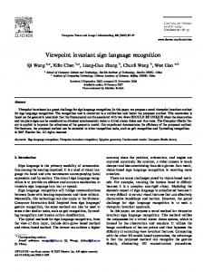
To avoid the modulus, the above formula can be written as a function of x 2 , y 2 and an exponent  [5]. We first consider the particular case when the scaling coefficients a and b are both 1. We call this initial family of shapes “supercircle” of unit radius (see Fig. 1):

 x2 + y 2 = 1 (1)

The addition of the single parameter  yields an interesting variety of shapes. Next we generalize this shape family to one that is closed under affine transformations, more precisely shapes that can be reduced to a supercircle via an affine transformation. The rationale is that as in the case of existing affine invariant regions, we want to find corresponding regions under variable viewpoints. These changes can be represented well by affine transformations. Hence, points xe on these shapes are found as: xe = Axc

(2)

where xc verifies the supercircle equation (1) and A is shorthand for the 3 × 3 affine transformation matrix. This family of shapes is wider than that of the original superellipses. Not only does it allow for rigid motions of the superellipses, but it also includes skewed versions, as exemplified in fig. 2. Applying affine transformations to superellipses rather than supercircles leads to exactly the same family, but with an overparameterized representation. We refer to the family as affine superellipses or ASEs for short. The parameter  provides a viewpoint independent shape parameter. If we can compose curves with a

Fig. 1. ”Supercircles” for different values of : 0.3, 0.5, 1, 2, 8

A A−1

P2 R2

R1

PSfrag replacements

P1 O2

O1

Fig. 2. Result of applying an affine transformation A to a supercircle.

small set of well fitting ASEs, the corresponding s and the ASEs’ configuration provide compact and viewpoint independent shape information. Fitting ASEs is the subject of the next section.

3 ASE fitting The problem of fitting superellipses is not entirely new. Rosin [14] has compared several objective functions to be minimized. These functions represent summed distances between the data points and selected points on the model curve. It proved difficult to choose one that would perform best in all cases. An important limitation was that contours were supposed to be closed. Fitting of an initial bounding box allowed him to immediately get rid of the translation and rotation components in the optimization. In a subsequent paper Zhang and Rosin [21] generalized the optimization to partial contours. They also mapped shapes back to the circle, as a normalization step prior to the evaluation of the objective function. The latter consisted of a sum of algebraic distances between the normalized contour and the circle, taking the local contour gradient and curvature into account. In our work, we have to deal with partial contours. We also add the skew parameter in order to deal with the full set of ASEs. Moreover, using the algebraic distance depends exponentially on . For example, considering the point (x, y) on the unit radius supercircle, the point (x + d, y) yields the error (x + d)2 − x2 . This means that rectangular shapes (   1) are more sensitive to outliers. Therefore, we use the Euclidean distance between contour points and the intersection of the ASE with the join through the point and the ASE’s center. Notice that this procedure does not normalize the ASE to a supercircle and, hence, the fitting procedure is not strictly affine invariant. We have found that prior normalization yields fitting results that are less robust, however. Some

PSfrag replacements

examples illustrating this are shown in fig. 3. We still need to study the precise causes in more depth. It should be noted that the Zhang and Rosin approach is also not affine invariant, even if they normalize, as they evenly sample the image contour before normalizing. Affine invariance wasn’t part of their goals. This sampling problem is shared by the PCA-based methods proposed by Pilu et al. [13], which deal with larger sets of deformations than affine, but only for closed contours.

O1 O2 R1 P1 R2 P2 A−1 A Fig. 3. Fitting superellipses to partial data. The red dashed lines represent the results of fitting using normalized distance, dotted green lines represent fitting using image distance. The original contours are gray. The segments used for fitting are drawn in black. In the last case the normalized version failed to converge.

With the notations from fig. 2, we minimize the sum of all squared Euclidean distances P2 R2 , where P2 represents a data point and R2 is the intersection between the ASE and the line passing through P2 and O2 - the ASE’s center: X D= |P2 − R2 |2 (3) P2 ∈data

The location of R2 is computed as follows:

R2 = AR1

(4)

where A is an affine matrix expressing the translation T , rotation R, scale S and skew K of the ASE: A = T RSK (5)     cos θ sin θ 0 1 0 tx T =  0 1 ty  ; R =  − sin θ cos θ 0  0 0 1 00 1     sx 0 0 1k0 S =  0 sy 0  ; K =  0 1 0  0 0 1 001

Switching to polar coordinates, R1 becomes:  xR1 = ρR1 cos θR1 R1 (ρ, θ) : yR1 = ρR1 sin θR1

(6)

R1 verifies the supercircle equation (1):
 

  =1 cos2 θR1 + sin2 θR1 ρ2R1 ⇔ ρ R1 =



cos2 θR1




+ sin2 θR1

P1 and R1 are colinear, so by replacing ( x cos θR1 = ρPP1 y 1 sin θR1 = ρPP1


  −1 2

(7) (8)

1

in equations (6) and (8), R1 can be written as a function of P1 and :  
 −1
  xR1 = xP 1 x2  + y 2  2 P1 P1 R1 = f (P1 , ) ⇔ 
 −1
 2  2 2  y = y + y x R1 P1 P1 P1

(9)

Also, P1 = A−1 P2 , so the expression of R2 is:

R2 = A f (A−1 P2 , ) Finally, the objective function has the following expression: X D= |P2 − A f (A−1 P2 , )|2

(10)

(11)

P2 ∈data

This being a nonlinear least-squares minimization problem, we applied the LevenbergMarquardt algorithm [20], a very effective and popular method for this category. The Levenberg-Marquardt algorithm requires an initial estimate of the objective function’s parameters, then proceeds iteratively towards the minimum. At each iteration it needs to evaluate the residual error and the function’s Jacobian matrix. The Jacobian has a quite complicated form, but the computations are straightforward so we omit them here. The  parameter is initialized to 2 and the skew to 0, while the other coefficients of the matrix A are initialized by an ellipse fitting algorithm [4]. The condition set for stopping the Levenberg-Marquardt algorithm is that for all of the 7 parameters the difference between successive iterations is less than 10−8 . On average less than 20 iterations are required for convergence. 3.1 Contour extraction An important issue is how the contours are extracted from natural images. Good contours are rather difficult to find, due to textures, occlusions, shadows, etc. For testing our algorithm we used a method introduced by Tuytelaars et al. [18]. Starting from a local extremum in the intensity K(x, y), rays are shot under different angles. The intensity pattern along each ray emanating from the extremum is studied by evaluating the function |K(t) − K0 |   fK (t) = Rt max d, 1t 0 |K(τ ) − K0 |dτ

with t being the Euclidean arc length along the ray, K(t) the intensity at position t, K0 the intensity extremum and d a small number added to prevent division by zero. The point at which this function reaches an extremum is invariant under the affine geometric and photometric transformations (given the ray). All points corresponding to an extremum of fK along the rays are linked to form a closed contour. These are the contours from which we select affine invariant segments and then fit ASEs against. 3.2 Selection of invariant contour segments When fitting to partial contours, there is a further issue that corresponding segments should be selected independent of viewpoint. This can be achieved by using simple, affine invariant criteria. One is illustrated in fig. 4. Starting from a point K, one can select a segment such that the chords from the point to each of the endpoints enclose replacements the samePSfrag area between them and the contour, i.e. A1 = A2 in fig. 4. There typically is O1 segments still. Demanding that the white triangle ∆KLM an infinite number of such 2 in the figure has the twoOareas summed (A1 + A2 = 2A1 = 2A2 ) reduces the number R 1 of such segments to a finite set of possibilities. These segments M - K - L are the ones P1 we have fitted the ASEs to. R2 P2

M

A−1 A A2

A1 + A 2

L

A1 K

Fig. 4. Automatic selection of a partial contour: Starting from K, the chords KL and KM are drawn such that the areas A1 and A2 are equal and the area of the KLM triangle is equal to A1 + A2 . The partial contour excludes the LM arc.

When fitting we also look at the error. Local minima are of particular importance, as they suggest segments out of which the complete contour can be composed in a highly compact way. This point will be illustrated in the next section, where we show ASE-fits to contours extracted from real images.

4 Experimental results 4.1 Synthetic data For testing the accuracy of the fitting module we generated noisy superellipses with different rotation, scaling, skew and epsilon coefficients. We fixed the horizontal scaling factor to 100, and modified the other parameters as follows: vertical scaling from 50 to

150 in 6 steps, rotation angle from 0 to π/2 in 30 steps, skew factor from -50 to 50 in 6 steps. For each combination we modified the value of  from 1 to 30 in increments of 1 and verified the absolute error of the recovered  for different noise levels. The noise was generated from a uniform distribution, having a spread of 0, 1, 2 and 4 pixels. Fitting was done using only half of the full contour. The coordinates of the generated points were rounded to integer coordinates. The plot of the standard deviation of the estimated  from the true value is shown in fig. 5. As can be seen, rectangular shapes (  1) are the worst affected by noise and rounding. This result is not surprising, since sharp corners become less clear as the noise increases. In the absence of noise and without rounding the coordinates to integers, the fitting PSfrag replacements procedure can recover the original  up to the fifth decimal. O1 O2 R1 P1 R2 P2 A−1 A K L M A1 A2 A1 + A 2

5 4.5 4 3.5 3 2.5 2 1.5 1 0.5 0

noise = 0 noise = 1 noise = 2 noise = 4

0

5

10

15

20

25

30

Fig. 5. Plot of the error of : The horizontal axis represents the ground truth . The vertical axis shows the standard deviation of the recovered .

4.2 Natural image contours Fig. 6 shows the back windows of a car, viewed from two directions. We show two types of ASEs that yield local minima for the fitting error. As can be seen, these correspond quite well, both between the mirror symmetric window pairs within each image, but also between the images. The overall shape can be represented efficiently as a combination of the two ASE types, as can be seen in the right column. The epsilon values are added in the figure and can be seen to be quite clustered. The difference in the values of  is caused by non-zero mean errors during the contour extraction. Similar examples can be seen in fig. 7, 8. Fig. 7 and 9 show ASEs fitted to the headlights of different cars. Again, as few as two ASEs manage to form a good approximation of these shapes. As one can see, in contrast to e.g. wheels, which always are elliptical with  = 1, head-lights are parts with a much wider variation in their shapes. As can also be seen from these examples, the pairs of head-lights are approximated by ASEs with similar epsilon values. Other examples are presented in fig. 10.

5 Conclusions and future work Currently, we are working on affine invariant descriptions of such ASE configurations, both in terms of their overall shape, as the texture content within their approximated contour. For the latter, already extensive sets of measures exist. Moment invariants would be one option [11]. As to the shape features, the ratio of areas of the different ASEs in the final configuration would be one simple, additional example. Other features should describe their relative positions, skews, and orientations. These can be quantified by normalizing one of the ASEs to a supercircle, and expressing these parameters with respect to the reference frame thus created. The results seem to corroborate the viability of the ASE approach. In its full-fledged form it will not only include several of the affine invariant region types already in use, but will also provide a link between the texture based methods that these basically are, and shape-based approaches. Indeed, it stands to reason that a truly generic recognition system will have to draw on both.

Acknowledgements The authors gratefully ackowledge support from EC Cognitive Systems project CogViSys and the fund for Scientific Research Flanders.

PSfrag replacements O1 O2 R1 P1 R2 P2 A−1 A K L M A1 A2 A1 + A 2 Fig. 6. A combination of two ASEs can approximate the rear window of a car.

PSfrag replacements O1 O2 R1 P1 R2 P2 A−1 A K L M A1 A2 A1 + A 2 Fig. 7. Car headlights represented with ASE combinations.

References 1. A. Baumberg: ”Reliable feature matching across widely separated views”, IEEE Computer Vision and Pattern Recognition, pp. 774-781, 2000. 2. M.C. Burl, M. Weber, T.K. Leung and P. Perona: ”Recognition of Visual Object Classes”, Chapter to appear in: From Segmentation to Interpretation and Back: Mathematical Methods in Computer Vision, Springer Verlag. 3. R. Fergus, P. Perona, A. Zisserman: ”Object Class Recognition by Unsupervised ScaleInvariant Learning”, Proc. Conf. on Computer Vision and Pattern Recognition - CVPR, IEEE, 2003. 4. A. Fitzgibbon, M. Pilu, R.B. Fisher: ”Direct least squares fitting of ellipses”, IEEE Transactions on Pattern Analysis and Machine Intelligence, Vol 21, Issue 5, pp. 476-480, May 1999. 5. M. Gardiner: ”The superellipse: a curve that lies between the ellipse and the rectangle”, Scientific American 21, pp. 222-234, 1965. 6. S.Helmer, D.Lowe: ”Object Recognition with Many Local Features.”, to appear at Generative Model Based Vision Workshop (CVPR 2004) 7. F.Jurie, C.Schmid: ”Scale-Invariant Features for Recognition of Object Categories.”, Proc. Conf on Computer Vision and Pattern Recognition - CVPR, IEEE, June 2004, Vol II, pp. 90-96. 8. S. Lazebnik, C. Schmid, J. Ponce: ”Affine-Invariant Local Descriptors and Neighborhood Statistics for Texture Recognition”, Proc. Conf. on Computer Vision, Nice, France - CVPR, IEEE, October 2003, pp. 649-655. 9. K. Mikolajczyk, C. Schmid: ”An affine invariant interest point detector”, European Conference on Computer Vision, Vol. 1, pp. 128-142, 2002. 10. K. Mikolajczyk, A. Zisserman, C. Schmid: ”Shape recognition with edge-based features”, Proc. of the British Machine Vision Conference - BMVC 2003 11. F. Mindru, T. Moons, L. Van Gool: ”Recognizing color patterns irrespective of viewpoint and illumination”, Proc. Conference on Computer Vision and Pattern Recognition - CVPR, IEEE, pp. 368-373, June 1999.

PSfrag replacements

PSfrag replacements

O1 O2 R1 P1 R2 P2 A−1 A PSfrag replacements K OL1 O M2 R1 A P21 A R2 A1 + A P2 A−1 A K L M A1 A2 A1 + A 2

O1 O2 R1 P1 R2 P2 A−1 A PSfrag replacements K OL1 O M2 R1 A P21 A R2 A1 + A P2 A−1 A K L M A1 A2 A1 + A 2

Fig. 8. Viewpoint invariance. Note that the bottom-right image is affected by projective errors, thus the rectangular window must be approximated by two ASEs.

12. S. Obdzalek, J.Matas: ”Object recognition using Local Affine Frames on Distinguished Regions”, British Machine Vision Conference, pp. 414-431, 2002. 13. M. Pilu, A.W. Fitzgibbon, R.B. Fisher: ”Training PDM on models: The case of deformable superellipses”, In Proceedings of the British Machine Vision Conference, Edinburgh, pp. 373382, September 1996. 14. P. Rosin: ”Fitting Superellipses”, IEEE Transactions on Pattern Analysis and Machine Intelligence, Vol 22, No. 7, July 2000. 15. F. Rothganger, S. Lazebnik, C. Schmid, J. Ponce: ”3D Object Modeling and Recognition Using Affine-Invariant Patches and Multi-View Spatial Constraints”, Proc. Conf on Computer Vision and Pattern Recognition - CVPR, IEEE, June 2003, Vol. II, pp. 272-277. 16. C. Schmid, R. Mohr: ”Local Grayvalue Invariants for Image Retrieval”, IEEE Transactions on Pattern Analysis and Machine Intelligence, 19(5), pp. 530-535, 1997. 17. D. Tell, S. Carlsson: ”Wide baseline point matching using affine invariants computed from intensity profiles”, ECCV, Vol. 1, pp. 814-828, 2000. 18. T. Tuytelaars, L.Van Gool: ”Wide baseline stereo matching based on local affinely invariant regions”, Proceedings British Machine Vision Conference, Sept.2000, pp. 412-422. 19. Eric W. Weisstein. ”Superellipse.” From MathWorld A Wolfram Web Resource. http://mathworld.wolfram.com/Superellipse.html 20. Eric W. Weisstein. ”Levenberg-Marquardt Method.” From MathWorld - A Wolfram Web Resource. http://mathworld.wolfram.com/LevenbergMarquardt Method.html 21. X. Zhang, P. Rosin: ”Superellipse fitting to partial data”, Pattern Recognition, No. 36, pp. 743-752, 2003.

PSfrag replacements O1 O2 R1 P1 R2 P2 A−1 A K L M A1 A2 A1 + A 2 Fig. 9. Other ASE combinations fitted to car headlights.

PSfrag replacements

PSfrag replacements

O1 O2 R1 P1 R2 P2

O1 O2 R1 P1 R2 P2

A−1 A K L M A1 A2 A1 + A 2

A−1 A K L M A1 A2 A1 + A 2

Fig. 10. Left: two pairs of glasses. Right: Detail of the headlight of a Mercedes.